Tropical Scaling of Polynomial Matrices

Abstract

The eigenvalues of a matrix polynomial can be determined classically by solving a generalized eigenproblem for a linearized matrix pencil, for instance by writing the matrix polynomial in companion form. We introduce a general scaling technique, based on tropical algebra, which applies in particular to this companion form. This scaling, which is inspired by an earlier work of Akian, Bapat, and Gaubert, relies on the computation of “tropical roots”. We give explicit bounds, in a typical case, indicating that these roots provide accurate estimates of the order of magnitude of the different eigenvalues, and we show by experiments that this scaling improves the accuracy (measured by normwise backward error) of the computations, particularly in situations in which the data have various orders of magnitude. In the case of quadratic polynomial matrices, we recover in this way a scaling due to Fan, Lin, and Van Dooren, which coincides with the tropical scaling when the two tropical roots are equal. If not, the eigenvalues generally split in two groups, and the tropical method leads to making one specific scaling for each of the groups.

1 Introduction

A classical problem is to compute the eigenvalues of a matrix polynomial

$$P(\lambda)=A_{0}+A_{1}\lambda+\cdots+A_{d}\lambda^{d}$$

where $A_{l}\in\mathbb{C}^{n\times n},l=0\ldots d$ are given. The eigenvalues are defined as the solutions of $\det(P(\lambda))=0$. If $\lambda$ is an eigenvalue, the associated right and left eigenvectors $x$ and $y\in\mathbb{C}^{n}$ are the non-zero solutions of the systems $P(\lambda)x=0$ and $y^{*}P(\lambda)=0$, respectively. A common way to solve this problem, is to convert $P$ into a “linearized” matrix pencil

$$L(\lambda)=\lambda X+Y,\quad X,Y\in\mathbb{C}^{nd\times nd}$$

with the same spectrum as $P$ and solve the eigenproblem for $L$, by standard numerical algorithms like the QZ method moler73 . If $D$ and $D^{\prime}$ are invertible diagonal matrices, and if $\alpha$ is a non-zero scalar, we may consider equivalently the scaled pencil $DL(\alpha\lambda)D^{\prime}$.

The problem of finding the good linearizations and the good scalings has received a considerable attention. The backward error and conditioning of the matrix pencil problem and of its linearizations have been investigated in particular in works of Tisseur, Li, Higham, and Mackey, see tisseur00 ; Higham061 ; Higham062 .

A scaling on the eigenvalue parameter to improve the normwise backward error of a quadratic polynomial matrix was proposed by Fan, Lin, and Van Dooren vandooren00 . This scaling only relies on the norms $\gamma_{l}:=\|A_{l}\|$, $l=0,1,2$. In this paper, we introduce a new family of scalings which also rely on these norms. The degree $d$ is now arbitrary.

These scalings originate from the work of Akian, Bapat, and Gaubert abg04b ; abg04 , in which the entries of the matrices $A_{l}$ are functions, for instance Puiseux series, of a (perturbation) parameter $t$. The valuations (leading exponents) of the Puiseux series representing the different eigenvalues were shown to coincide, under some genericity conditions, with the points of non-differentiability of the value function of a parametric optimal assignment problem (the tropical eigenvalues), a result which can be interpreted in terms of amoebas itenberg . Indeed, the definition of the tropical eigenvalues in abg04b ; abg04 makes sense in any field with valuation. In particular, when the coefficients belong to $\mathbb{C}$, we can take the map $z\mapsto\log|z|$ from $\mathbb{C}$ to $\mathbb{R}\cup\{-\infty\}$ as the valuation. Then, the tropical eigenvalues are expected to give, again under some non degeneracy conditions, the correct order of magnitude of the different eigenvalues.

The tropical roots used in the present paper are an approximation of the tropical eigenvalues, relying only on the norms $\gamma_{l}=\|A_{l}\|$. A better scaling may be achieved by considering the tropical eigenvalues, but computing these eigenvalues requires $O(nd)$ calls to an optimal assignment algorithm, whereas the tropical roots considered here can be computed in $O(d)$ time, see Remark 3 below for more information. We examine such extensions in a further work.

As an illustration, consider the following quadratic polynomial matrix

$$P(\lambda)=\lambda^{2}10^{-18}\begin{pmatrix}1&2\\ 3&4\end{pmatrix}+\lambda\begin{pmatrix}-3&10\\ 16&45\end{pmatrix}+10^{-18}\begin{pmatrix}12&15\\ 34&28\end{pmatrix}$$

By applying the QZ algorithm on the first companion form of $P(\lambda)$ we get the eigenvalues -Inf,- 7.731e-19 , Inf, 3.588e-19, by using the scaling proposed in  vandooren00 we get -Inf, -3.250e-19, Inf, 3.588e-19. However by using the tropical scaling we can find the four eigenvalues properly: - 7.250e-18 $\pm$ 9.744e-18i, - 2.102e+17 $\pm$ 7.387e+17i. The result was shown to be correct (actually, up to a 14 digits precision) with PARI, in which an arbitrarily large precision can be set. The above computations were performed in Matlab (version 7.3.0).

The paper is organized as follows. In Section 2, we recall some classical facts of max-plus or tropical algebra, and show that the tropical roots of a tropical polynomial can be computed in linear time, using a convex hull algorithm. Section 3 states preliminary results concerning matrix pencils, linearization and normwise backward error.

In Section 4, we describe our scaling method. In Section 5, we give a theorem locating the eigenvalues of a quadratic polynomial matrix, which provides some theoretical justification of the method. Finally in Section 6, we present the experimental results showing that the tropical scaling can highly reduce the normwise backward error of an eigenpair. We consider the quadratic case in Section 6.1 and the general case in Section 6.2. For the quadratic case, we compare our results with the scaling proposed in  vandooren00 .

2 Tropical polynomials

The max-plus semiring $\mathbb{R}_{\max}$, is the set $\mathbb{R}\cup\{-\infty\}$, equipped with max as addition, and the usual addition as multiplication. It is traditional to use the notation $\oplus$ for $\max$ (so $2\oplus 3=3$), and $\otimes$ for $+$ (so $1\otimes 1=2$). We denote by $\mathbb{0}$ the zero element of the semiring, which is such that $\mathbb{0}\oplus a=a$, here $\mathbb{0}=-\infty$, and by $\mathbb{1}$ the unit element of the semiring, which is such that $\mathbb{1}\otimes a=a\otimes\mathbb{1}=a$, here $\mathbb{1}=0$. We refer the reader to BCOQ92 ; KM ; AG for more background.

A variant of this semiring is the max-times semiring $\mathbb{R}_{\max,\times}$, which is the set of nonnegative real numbers $\mathbb{R}^{+}$, equipped with max as addition, and $\times$ as multiplication. This semiring is isomorphic to $\mathbb{R}_{\max}$ by the map $x\mapsto\log x$. So, every notion defined over $\mathbb{R}_{\max}$ has an $\mathbb{R}_{\max,\times}$ analogue that we shall not redefine explicitly. In the sequel, the word “tropical” will refer indifferently to any of these algebraic structures.

Consider a max-plus (formal) polynomial of degree $n$ in one variable, i.e., a formal expression $P=\bigoplus_{0\leq k\leq n}P_{k}X^{k}$ in which the coefficients $P_{k}$ belong to $\mathbb{R}_{\max}$, and the associated numerical polynomial, which, with the notation of the classical algebra, can be written as $p(x)=\max_{0\leq k\leq n}P_{k}+kx$. Cuninghame-Green and Meijer showed cuning80 that the analogue of the fundamental theorem of algebra holds in the max-plus setting, i.e., that $p(x)$ can be written uniquely as $p(x)=P_{n}+\sum_{1\leq k\leq n}\max(x,c_{k})$, where $c_{1},\ldots,c_{n}\in\mathbb{R}_{\max}$ are the roots, i.e., the points at which the maximum attained at least twice. This is a special case of more general notions which have arisen recently in tropical geometry itenberg . The multiplicity of the root $c$ is the cardinality of the set $\{k\in\{1,\ldots,n\}\mid c_{k}=c\}$. Define the Newton polygon $\Delta(P)$ of $P$ to be the upper boundary of the convex hull of the set of points $(k,P_{k})$, $k=0,\ldots,n$. This boundary consists of a number of linear segments. An application of Legendre-Fenchel duality (see (abg04b, , Proposition 2.10)) shows that the opposite of the slopes of these segments are precisely the tropical roots, and that the multiplicity of a root coincides with the horizontal width of the corresponding segment. (Actually, min-plus polynomials are considered in abg04b , but the max-plus case reduces to the min-plus case by an obvious change of variable). Since the Graham scan algorithm Graham72 allows us to compute the convex hull of a finite set of points by making $O(n)$ arithmetical operations and comparisons, provided that the given set of points is already sorted by abscissa, we get the following result.

Proposition 1

The roots of a max-plus polynomial in one variable can be computed in linear time. ∎

The case of a max-times polynomial reduces to the max-plus case by replacing every coefficient by its logarithm. The exponentials of the roots of the transformed polynomial are the roots of the original polynomial.

3 Matrix pencil and normwise backward error

Let us come back to the eigenvalue problem for the matrix pencil $P(\lambda)=A_{0}+A_{1}\lambda+\cdots+A_{d}\lambda^{d}$. There are many ways to construct a “linearized” matrix pencil $L(\lambda)=\lambda X+Y,\quad X,Y\in\mathbb{C}^{nd\times nd}$ with the same spectrum as $P(\lambda)$, see Mackey06 for a general discussion. In particular, the first companion form $\lambda X_{1}+Y_{1}$ is defined by

$$X_{1}=\operatorname{diag}(A_{k},I_{(k-1)n}),\qquad Y_{1}=\begin{pmatrix}A_{k-1}&A_{k-2}&\ldots&A_{0}\\ -I_{n}&0&\ldots&0\\ \vdots&\vdots&\vdots&\ddots\\ 0&\ldots&-I_{n}&0\end{pmatrix}\enspace.$$

In the experimental part of this work, we are using this linearization.

To estimate the accuracy of a numerical algorithm computing an eigenpair, we shall consider, as in tisseur00 , the normwise backward error. The latter arises when considering a perturbation

$$\Delta P=\Delta A_{0}+\Delta A_{1}\lambda+\cdots+\Delta A_{d}\lambda^{d}\enspace.$$

The backward error of an approximate eigenpair $(\tilde{x},\tilde{\lambda})$ of $P$ is defined by

$$\eta(\tilde{x},\tilde{\lambda})=\min\{\epsilon:(P(\tilde{\lambda})+\Delta P(\tilde{\lambda}))\tilde{x}=0,\|\Delta A_{l}\|_{2}\leq\epsilon\|E_{l}\|_{2},l=0,\ldots m\}\enspace.$$

The matrices $E_{l}$ representing tolerances. The following computable expression for $\eta(\tilde{x},\tilde{\lambda})$ is given in the same reference,

$$\eta(\tilde{x},\tilde{\lambda})=\frac{\|r\|_{2}}{\tilde{\alpha}\|\tilde{x}\|_{2}}$$

where $r=P(\tilde{\lambda})\tilde{x}$ and $\tilde{\alpha}=\sum{|\tilde{\lambda}|^{l}\|E_{l}\|_{2}}$. In the sequel, we shall take $E_{l}=A_{l}$.

Our aim is to reduce the normwise backward error, by a scaling of the eigenvalue $\lambda=\alpha\mu$, where $\alpha$ is the scaling parameter. This kind of scaling for quadratic polynomial matrix was proposed by Fan, Lin and Van Dooren vandooren00 . We next introduce a new scaling, based on the tropical roots.

4 Construction of the tropical scaling

Consider the matrix pencil modified by the substitution $\lambda=\alpha\mu$

$$\tilde{P}(\mu)=\tilde{A}_{0}+\tilde{A}_{1}\mu+\cdots+\tilde{A}_{d}\mu^{d}$$

where $\tilde{A}_{i}=\beta\alpha^{i}{A}_{i}$.

The tropical scaling which we next introduce is characterized by the property that $\alpha$ and $\beta$ are such that $\tilde{P}(\mu)$ has at least two matrices $\tilde{A}_{i}$ with an (induced) Euclidean norm equal to one, whereas the Euclidean norm of the other matrices are all bounded by one. This scaling is inspired by the work of M. Akian and R. Bapat and S. Gaubert abg04 , which concerns the perturbation of the eigenvalues of a matrix pencil. The theorem on the location of the eigenvalues which is stated in the next section provides some justification for the present scaling.

We associate to the original pencil the max-times polynomial

$$\mathsf{t}p(x)=\max(\gamma_{0},\gamma_{1}\lambda,\cdots,\gamma_{d}\lambda^{d})\enspace,$$

where

$$\gamma_{i}:=\|A_{i}\|$$

(the symbol $\mathsf{t}$ stands for “tropical”). Let $\alpha_{1}\leq\alpha_{2}\leq\ldots\leq\alpha_{d}$ be the tropical roots of $\mathsf{t}p(x)$ counted with multiplicities. For each $\alpha_{i}$, the maximum is attained by at least two mononomials. Subsequently, the transformed polynomial $q(x):=\beta_{i}\mathsf{t}p(\alpha_{i}x)$, with $\beta_{i}:=(\mathsf{t}p(\alpha_{i}))^{-1}$ has two coefficients of modulus one, and all the other coefficients have modulus less than or equal to one. Thus $\alpha=\alpha_{i}$ and $\beta=\beta_{i}$ will satisfy the goal.

The idea is to apply this scaling for all the tropical roots of $\mathsf{t}p(x)$ and each time, to compute $n$ out of $nd$ eigenvalues of the corresponding scaled matrix pencil, because replacing $P(\lambda)$ by $P(\alpha_{i}\mu)$ is expected to decrease the backward error for the eigenvalues of order $\alpha_{i}$, while possibly increasing the backward error for the other ones.

More precisely, let $\alpha_{1}\leq\alpha_{1}\leq\ldots\leq\alpha_{d}$ denote the tropical roots of $\mathsf{t}p(x)$. Also let

$$\underbrace{\mu_{1},\ldots,\mu_{n}},\underbrace{\mu_{n+1},\ldots,\mu_{2n}},\ldots,\underbrace{\mu_{(d-1)n+1},\ldots,\mu_{nd}}$$

be the eigenvalues of $\tilde{P}(\mu)$ sorted by increasing modulus, computed by setting $\alpha=\alpha_{i}$ and $\beta=\mathsf{t}p(\alpha_{i})^{-1}$ and partitioned in $d$ different groups. Now, we choose the $i$th group of $n$ eigenvalues, multiply by $\alpha_{i}$ and put in the list of computed eigenvalues. By applying this iteration for all $i=1\ldots d$, we will get the list of the eigenvalues of $P(\lambda)$. Taking into account this description, we arrive at Algorithm 1. It should be understood here that in the sequence $\mu_{1},\ldots,\mu_{nd}$ of eigenvalues above, only the eigenvalues of order $\alpha_{i}$ are hoped to be computed accurately. Indeed, in some extreme cases in which the tropical roots have very different orders of magnitude (as in the example shown in the introduction), the eigenvalues of order $\alpha_{i}$ turn out to be accurate whereas the groups of higher orders have some eigenvalues Inf or Nan. So, Algorithm 1 merges into a single picture several snapshots of the spectrum, each of them being accurate on a different part of the spectrum.

Algorithm 1 Computing the eigenvalues using the tropical scaling
INPUT: Matrix pencil $P(\lambda)$
OUTPUT: List of eigenvalues of $P(\lambda)$
1.	Compute the corresponding tropical polynomial $\mathsf{t}p(x)$
2.	Find the tropical roots of $\mathsf{t}p(x)$
3.	For each tropical root such as $\alpha_{i}$ do
	3.1	Compute the tropical scaling based on $\alpha_{i}$
	3.2	Compute the eigenvalues using the QZ algorithm
		and sort them by increasing modulus
	3.3	Choose the $i$th group of the eigenvalues

To illustrate the algorithm, let $P(\lambda)=A_{0}+A_{1}\lambda+A_{2}\lambda^{2}$ be a quadratic polynomial matrix and let $\mathsf{t}p(\lambda)=\max(\gamma_{0},\gamma_{1}\lambda,\gamma_{2}\lambda^{2})$ be the tropical polynomial corresponding to this quadratic polynomial matrix.

We refer to the tropical roots of $\mathsf{t}p(x)$ by $\alpha^{+}\geq\alpha^{-}$. If $\alpha^{+}=\alpha^{-}$ which happens when $\gamma_{1}^{2}\leq\gamma_{0}\gamma_{2}$ then, $\alpha=\sqrt{\frac{\gamma_{0}}{\gamma_{2}}}$ and $\beta=\mathsf{t}p(\alpha)^{-1}=\gamma_{0}^{-1}$. This case coincides with the scaling of vandooren00 in which $\alpha^{*}=\sqrt{\frac{\gamma_{0}}{\gamma_{2}}}$.

When $\alpha^{+}\neq\alpha^{-}$, we will have two different scalings based on $\alpha^{+}=\frac{\gamma_{1}}{\gamma_{2}}$, $\alpha^{-}=\frac{\gamma_{0}}{\gamma_{1}}$ and two different $\beta$ corresponding to the two tropical roots:

$$\beta^{+}=\mathsf{t}p(\alpha^{+})^{-1}=\frac{\gamma_{2}}{\gamma_{1}^{2}},\qquad\beta^{-}=\mathsf{t}p(\alpha^{-})^{-1}=\frac{1}{\gamma_{0}}.$$

To compute the eigenvalues of $P(\lambda)$ by using the first companion form linearization, we apply the scaling based on $\alpha^{+}$, which yields

$$\lambda\begin{pmatrix}\frac{1}{\gamma_{2}}A_{2}&\\ &I\end{pmatrix}+\begin{pmatrix}\frac{1}{\gamma_{1}}A_{1}&\frac{\gamma_{2}}{\gamma_{1}^{2}}A_{0}\\ -I&0\end{pmatrix}\enspace,$$

to compute the $n$ biggest eigenvalues. We apply the scaling based on $\alpha^{-}$, which yields

$$\lambda\begin{pmatrix}\frac{\gamma_{0}}{\gamma_{1}^{2}}A_{2}&\\ &I\end{pmatrix}+\begin{pmatrix}\frac{1}{\gamma_{1}}A_{1}&\frac{1}{\gamma_{2}}A_{0}\\ -I&0\end{pmatrix}\enspace,$$

to compute the $n$ smallest eigenvalues.

In general, let $\alpha_{1}\leq\alpha_{1}\leq\ldots\leq\alpha_{d}$ be the tropical roots of $\mathsf{t}p(x)$ counted with multiplicities. To compute the $i$th biggest group of eigenvalues, we perform the scaling for $\alpha_{i}$, which yields the following linearization:

$$\lambda\begin{pmatrix}\beta\alpha_{i}^{d}A_{d}&\\ &I\\ &&\ddots\\ &&&I\\ &&&&I\end{pmatrix}+\begin{pmatrix}\beta\alpha_{i}^{d-1}A_{d-1}&\ldots&\beta\alpha_{i}A_{1}&\beta A_{0}\\ -I&0&\ldots&0\\ 0&-I&\ddots&\vdots\\ \vdots&&\ddots&0\\ 0&\ldots&-I&0\end{pmatrix}$$

where $\beta=\mathsf{t}p(\alpha_{i})^{-1}$. Doing the same for all the distinct tropical roots, we can compute all the eigenvalues.

Remark 1

The interest of Algorithm 1 lies in the accuracy (since it allows us to solve instances in which the data have various order of magnitudes). Its inconvenient is to call several times (once for each distinct tropical eigenvalue, and so, at most $d$ times) the QZ algorithm. However, we may partition the different tropical eigenvalues in groups consisting each of eigenvalues of the same order of magnitude, and then, the speed factor we would loose would be reduced to the number of different groups.

5 Splitting of the eigenvalues in tropical groups

In this section we state a simple theorem concerning the location of the eigenvalues of a quadratic polynomial matrix, showing that under a non degeneracy condition, the two tropical roots do provide the correct estimate of the modulus of the eigenvalues.

We shall need to compare spectra, which may be thought of as unordered sets, therefore, we define the following metric (eigenvalue variation), which appeared in Gal08 . We shall use the notation $\operatorname{spec}$ for the spectrum of a matrix or a pencil.

Definition 1

Let $\lambda_{1},\ldots\lambda_{n}$ and $\mu_{1}\ldots\mu_{n}$ denote two sequences of complex numbers. The variation between $\lambda$ and $\mu$ is defined by

$$v(\lambda,\mu):=\min_{\pi\in S_{n}}\{\max_{i}|\mu_{\pi(i)}-\lambda_{i}|\}\enspace,$$

where $S_{n}$ is the set of permutations of $\{1,2,\ldots,n\}$. If $A,B\in\mathbb{C}^{n\times n}$, the eigenvalue variation of $A$ and $B$ is defined by $v(A,B):=v(\operatorname{spec}A,\operatorname{spec}B)$.

Recall that the quantity $v(\lambda,\mu)$ can be computed in polynomial time by solving a bottleneck assignment problem.

We shall need the following theorem of Bathia, Elsner, and Krause bhatia .

Theorem 5.1 (bhatia )

Let $A,B\in\mathbb{C}^{n\times n}$. Then $v(A,B)\leq 4\times 2^{-1/n}(\|A\|+\|B\|)^{1-1/n}\|A-B\|^{1/n}$ .

The following result shows that when the parameter $\delta$ measuring the separation between the two tropical roots is sufficiently large, and when the matrices $A_{2},A_{1}$ are well conditioned, then, there are precisely $n$ eigenvalues of the order of the maximal tropical root. By applying the same result to the reciprocal pencil, we deduce, under the same separation condition, that when $A_{1},A_{0}$ are well conditioned, there are precisely $n$ eigenvalues of the order of the minimal tropical root. So, under such conditions, the tropical roots provide accurate a priori estimates of the order of the eigenvalues of the pencil.

Theorem 5.2 (Tropical splitting of eigenvalues)

Let $P(\lambda)=\lambda^{2}A_{2}+\lambda A_{1}+A_{0}$ where $A_{i}\in\mathbb{C}^{n\times n}$, and $\gamma_{i}:=\|A_{i}\|$, $i=0,1,2$. Assume that the max-times polynomial $p(\lambda)=\max(\lambda^{2}\gamma_{2},\lambda\gamma_{1},\gamma_{0})$ has two distinct tropical roots, $\alpha^{+}:=\gamma_{1}/\gamma_{2}$ and $\alpha^{-}=\gamma_{0}/\gamma_{1}$, and let $\delta:=\alpha^{+}/\alpha^{-}$. Assume that $A_{2}$ is invertible. Let $\xi_{1},\ldots,\xi_{n}$ denote the eigenvalues of the pencil $\lambda A_{2}+A_{1}$, and let us set $\xi_{n+1}=\cdots=\xi_{2n}=0$. Then,

$$v(\operatorname{spec}P,\xi)\leq\frac{C\alpha^{+}}{\delta^{1/2n}}\enspace,$$

where

$$C:=4\times 2^{-1/2n}\big{(}2+2\operatorname{cond}A_{2}+\frac{\operatorname{cond}A_{2}}{\delta}\big{)}^{1-1/2n}\big{(}\operatorname{cond}A_{2}\big{)}^{1/2n}\enspace,$$

and

$$\alpha^{+}(\operatorname{cond}A_{1})^{-1}\leq|\xi_{i}|\leq\alpha^{+}\operatorname{cond}A_{2},\qquad 1\leq i\leq n\enspace.$$ (1)

Proof

Let us make the scaling corresponding to the maximal tropical root $\alpha^{+}=\gamma_{1}/\gamma_{2}$, with $\beta^{+}=\gamma_{2}/\gamma_{1}^{2}$, which amounts to considering the new polynomial matrix $Q(\mu)=\beta^{+}P(\alpha^{+}\mu)=\bar{A}_{2}\mu^{2}+\bar{A}_{1}\mu+\bar{A}_{0}$ where

$$\bar{A}_{2}=\gamma_{2}^{-1}A_{2},\qquad\bar{A}_{1}=\gamma_{1}^{-1}A_{1},\qquad\bar{A}_{0}=\frac{\gamma_{2}}{\gamma_{1}^{2}}A_{0}\enspace.$$

Since $A_{2}$ is invertible, $\lambda$ is an eigenvalue of the pencil $P$ if and only if $\lambda=\alpha^{+}\mu$ where $\mu$ is an eigenvalue of the matrix:

$$X=\begin{pmatrix}-\bar{A}_{2}^{-1}\bar{A}_{1}&-\bar{A}_{2}^{-1}\bar{A}_{0}\\ I&0\end{pmatrix}$$

Let $\mu_{i},i=1,\ldots,2n$ denote the eigenvalues of this matrix. Consider

$$Y=\begin{pmatrix}-\bar{A}_{2}^{-1}\bar{A}_{1}&0\\ I&0\end{pmatrix}$$

Observe that $\|\bar{A}_{1}\|=1$ and $\|\bar{A}_{0}\|=\gamma_{2}\gamma_{0}/\gamma_{1}^{2}=1/\delta$. Since the induced Euclidean norm $\|\cdot\|$ is an algebra norm, we get

$$\|X\|\leq\|I\|+\|\bar{A}_{2}^{-1}\bar{A}_{1}\|+\|\bar{A}_{2}^{-1}\bar{A}_{0}\| \leq 1+\|A_{2}^{-1}\|\|A_{2}\|+\|A_{2}^{-1}\|\|A_{2}\|\|\bar{A}_{0}\|$$

$$=1+\operatorname{cond}A_{2}(1+1/\delta)\enspace.$$

Moreover,

$$\|Y\|\leq 1+\operatorname{cond}A_{2}\enspace,\qquad\|X-Y\|=(\operatorname{cond}A_{2})/\delta.$$

Using Theorem 5.1, we deduce that

$$v(\operatorname{spec}X,\operatorname{spec}Y)\leq C/\delta^{1/2n}\enspace.$$

Since the family of eigenvalues of $P$ coincide with $\alpha^{+}(\operatorname{spec}X)$, and since the family of numbers $\xi_{i}$ coincides with $\alpha^{+}(\operatorname{spec}Y)$, the first part of the result is proved.

If $\xi$ is an eigenvalue of $A_{2}\lambda+A_{1}$, then, we can write $\xi=\alpha^{+}\zeta$, where $\zeta$ is an eigenvalue of $\bar{A}_{2}\mu+\bar{A}_{1}$. We deduce that $|\zeta|\leq\|\bar{A}_{2}^{-1}\|\|\bar{A}_{1}\|=\operatorname{cond}A_{2}$, which establishes the second inequality in (1). The first inequality is established along the same lines, by considering the reciprocal pencil of $\bar{A}_{2}\mu+\bar{A}_{1}$. ∎

Remark 2

Theorem 5.2 is a typical, but special instance of a general class of results that we discuss in a further work. In particular, this theorem can be extended to matrix polynomials of an arbitrary degree, with a different proof technique. Indeed, the idea of the proof above works only for the two “extreme” groups of eigenvalues, whereas in the degree $d$ case, the eigenvalues are split in $d$ groups (still under nondegeneracy conditions). Note also that the exponent in $\delta^{1/2n}$ is suboptimal

Remark 3

In abg04 ; abg04b , the tropical eigenvalues are defined as follows. The permanent of a $n\times n$ matrix $B=(b_{ij})$ with entries in $\mathbb{R}_{\max}$ is defined by

$$\operatorname{per}B:=\max_{\sigma\in S_{n}}\sum_{1\leq i\leq n}b_{i\sigma(i)}\enspace.$$

This is nothing than the value of the optimal assignment problem with weights $(b_{ij})$. The characteristic polynomial of a matrix $C=(c_{ij})$ is defined as the map from $\mathbb{R}_{\max}$ to itself,

$$x\mapsto P_{C}(x):=\operatorname{per}(C\oplus xI)\enspace,$$

where $I$ is the max-plus identity matrix, with diagonal entries equal to $0$ and off-diagonal entries equal to $-\infty$. The sum $C\oplus xI$ is interpreted in the max-plus sense, so

$$(C\oplus xI)_{ij}=\begin{cases}c_{ij}&\text{if $i\neq j$}\\ \max(c_{ii},x)&\text{if $i=j$.}\end{cases}$$

The tropical eigenvalues are defined as the roots of the characteristic polynomial. The previous definition has an obvious generalization to the case of tropical matrix polynomials: if $C_{0},\ldots,C_{d}$ are $n\times n$ matrices with entries in $\mathbb{R}_{\max}$, the eigenvalues of the matrix polynomial $C(x):=C_{0}\oplus C_{1}x\oplus\cdots\oplus C_{d}x^{d}$ are defined as the roots of the polynomial function $x\mapsto\operatorname{per}(C(x))$. The roots of this function can be computed in polynomial time by $O(nd)$ calls to an optimal assignment solver (the case in which $C(x)=C_{0}\oplus xI$ was solved by Burkard and Butkovič bb02 ; the generalization to the degree $d$ case was pointed out in abg04 ). When the matrices $A_{0},\ldots,A_{d}$ are scalars, the logarithms of the tropical roots considered in the present paper are readily seen to coincide with the tropical eigenvalues of the pencil in which $C_{k}$ is the logarithm of the modulus of $A_{k}$, for $0\leq k\leq d$. When these matrices are not scalars, in view of the asymptotic results of abg04 , the exponentials of the tropical eigenvalues are expected to provide more accurate estimates of the moduli of the complex roots. This alternative approach is the object of a further work, however, the comparative interest of the tropical roots considered here lies in their simplicity: they only depend on the norms of $A_{0},\ldots,A_{d}$, and can be computed in linear time from these norms. They can also be used as a measure of ill-posedness of the problem (when the tropical roots have different orders of magnitude, the standard methods in general fail).

6 Experimental Results

6.1 Quadratic Polynomial Matrices

Consider first $P(\lambda)=A_{0}+A_{1}\lambda+A_{2}\lambda^{2}$ and its linearization $L=\lambda X+Y$. Let $z$ be the eigenvector computed by applying the QZ algorithm to this linearization. Both $\zeta_{1}=z(1:n)$ and $\zeta_{2}=z(n+1:2n)$ are eigenvectors of $P(\lambda)$. We present our results for both of these eigenvectors; $\eta_{s}$ denotes the normwise backward error for the scaling of vandooren00 , and $\eta_{t}$ denotes the same quantity for the tropical scaling.

Our first example coincides with Example 3 of vandooren00 where $\|A_{2}\|_{2}\approx 5.54\times 10^{-5},\|A_{1}\|_{2}\approx 4.73\times 10^{3},\|A_{0}\|_{2}\approx 6.01\times 10^{-3}$ and $A_{i}\in\mathbb{C}^{10\times 10}$. We used $100$ randomly generated pencils normalized to get the mentioned norms and we computed the average of the quantities mentioned in the following table for these pencils. Here we present the results for the $5$ smallest eigenvalues, however for all the eigenvalues, the backward error computed by using the tropical scaling is of order $10^{-16}$ which is the precision of the computation. The computations were carried out in SCILAB 4.1.2.

$|\lambda|$	$\eta(\zeta_{1},\lambda)$	$\eta(\zeta_{2},\lambda)$	$\eta_{s}(\zeta_{1},\lambda)$	$\eta_{s}(\zeta_{2},\lambda)$	$\eta_{t}(\zeta_{1},\lambda)$	$\eta_{t}(\zeta_{2},\lambda)$
2.98E-07	1.01E-06	4.13E-08	5.66E-09	5.27E-10	6.99E-16	1.90E-16
5.18E-07	1.37E-07	3.84E-08	8.48E-10	4.59E-10	2.72E-16	1.83E-16
7.38E-07	5.81E-08	2.92E-08	4.59E-10	3.91E-10	2.31E-16	1.71E-16
9.53E-07	3.79E-08	2.31E-08	3.47E-10	3.36E-10	2.08E-16	1.63E-16
1.24E-06	3.26E-08	2.64E-08	3.00E-10	3.23E-10	1.98E-16	1.74E-16

In the second example, we consider a matrix pencil with $\|A_{2}\|_{2}\approx 10^{-6},\|A_{1}\|_{2}\approx 10^{3},\|A_{0}\|_{2}\approx 10^{5}$ and $A_{i}\in\mathbb{C}^{40\times 40}$. Again, we use $100$ randomly generated pencils with the mentioned norms and we compute the average of all the quantities presented in the next table. We present the results for the $5$ smallest eigenvalues. This time, the computations shown are from MATLAB 7.3.0, actually, the results are insensitive to this choice, since the versions of MATLAB and SCILAB we used both rely on the QZ algorithm of Lapack library (version 3.0).

$|\lambda|$	$\eta(\zeta_{1},\lambda)$	$\eta(\zeta_{2},\lambda)$	$\eta_{s}(\zeta_{1},\lambda)$	$\eta_{s}(\zeta_{2},\lambda)$	$\eta_{T}(\zeta_{1},\lambda)$	$\eta_{T}(\zeta_{2},\lambda)$
1.08E+01	2.13E-13	4.97E-15	8.98E-12	4.19E-13	5.37E-15	3.99E-16
1.75E+01	5.20E-14	4.85E-15	7.71E-13	4.09E-13	6.76E-16	3.95E-16
2.35E+01	4.56E-14	5.25E-15	6.02E-13	4.01E-13	5.54E-16	3.66E-16
2.93E+01	4.18E-14	5.99E-15	5.03E-13	3.97E-13	4.80E-16	3.47E-16
3.33E+01	3.77E-14	5.28E-15	4.52E-13	3.84E-13	4.67E-16	3.53E-16

6.2 Polynomial Matrices of Degree $d$

Consider now the polynomial matrix $P(\lambda)=A_{0}+A_{1}\lambda+\cdots+A_{d}\lambda^{d}$, and let $L=\lambda X+Y$ be the first companion form linearization of this pencil. If $z$ is an eigenvector for $L$ then $\zeta_{1}=z(1:n)$ is an eigenvector for $P(\lambda)$. In the following computations, we use $\zeta_{1}$ to compute the normwise backward error of Matrix pencil, however this is possible to use any $z(kn+1:n(k+1))$ for $k=0\ldots d-1$.

To illustrate our results, we apply the algorithm for $20$ different randomly generated matrix pencils and then compute the backward error for a specific eigenvalue of these matrix pencils. The 20 values x-axis, in Fig. 2 and 2, identify the random instance while the y-axis shows the $\log_{10}$ of backward error for a specific eigenvalue. Also we sort the eigenvalues in a decreasing order of their absolute value, so $\lambda_{1}$ is the maximum eigenvalue.

We firstly consider the randomly generated matrix pencils of degree $5$ where the order of magnitude of the Euclidean norm of $A_{i}$ is as follows:

$\|A_{0}\|$	$\|A_{1}\|$	$\|A_{2}\|$	$\|A_{3}\|$	$\|A_{4}\|$	$\|A_{5}\|$
$O(10^{-3})$	$O(10^{2})$	$O(10^{2})$	$O(10^{-1})$	$O(10^{-4})$	$O(10^{5})$

Fig. 2 shows the results for this case where the dotted line shows the backward error without scaling and the solid line shows the backward error using the tropical scaling. We show the results for the minimum eigenvalue, the “central” $50^{\text{th}}$ eigenvalue and the maximum one from top to down. In particular, the picture at the top shows a dramatic improvement since the smallest of the eigenvalues is not computed accurately (backward error almost of order one) without the scaling, whereas for the biggest of the eigenvalues, the scaling typically improves the backward error by a factor 10. For the central eigenvalue, the improvement we get is intermediate. The second example concerns the randomly generated matrix pencil with degree $10$ while the order of the norm of the coefficient matrices are as follows:

$\|A_{0}\|$	$\|A_{1}\|$	$\|A_{2}\|$	$\|A_{3}\|$	$\|A_{4}\|$	$\|A_{5}\|$
$O(10^{-5})$	$O(10^{-2})$	$O(10^{-3})$	$O(10^{-4})$	$O(10^{2})$	$O(1)$

$\|A_{6}\|$	$\|A_{7}\|$	$\|A_{8}\|$	$\|A_{9}\|$	$\|A_{10}\|$
$O(10^{3})$	$O(10^{-3})$	$O(10^{4})$	$O(10^{2})$	$O(10^{5})$

In this example, the order of the norms differ from $10^{-5}$ to $10^{5}$ and the space dimension of $A_{i}$ is $8$. Figure  2 shows the results for this case where the dotted line shows the backward error without scaling and the solid line shows the backward error using tropical scaling. Again we show the results for the minimum eigenvalue, the $40$th eigenvalue and the maximum one from top to down.

Figure 1: Backward error for randomly generated matrix pencils with $n=20$, $d=5$.

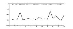
Figure 2: Backward error for randomly generated matrix pencils with $n=8$, $d=10$.

References

- (1) M. Akian, R. Bapat, and S. Gaubert. Perturbation of eigenvalues of matrix pencils and optimal assignment problem. C. R. Acad. Sci. Paris, Série I, 339:103–108, 2004. Also arXiv:math.SP/0402438.
- (2) M. Akian, R. Bapat, and S. Gaubert. Min-plus methods in eigenvalue perturbation theory and generalised Lidskii-Vishik-Ljusternik theorem. arXiv:math.SP/0402090, 2005.
- (3) M. Akian, R. Bapat, and S. Gaubert. Max-plus algebras. In L. Hogben, editor, Handbook of Linear Algebra (Discrete Mathematics and Its Applications), volume 39. Chapman & Hall/CRC, 2006. Chapter 25.
- (4) F. Baccelli, G. Cohen, G.J. Olsder, and J.P. Quadrat. Synchronization and Linearity. Wiley, 1992.
- (5) R. Bhatia, L. Elsner, and G. Krause. Bounds for the variation of the roots of a polynomial and the eigenvalues of a matrix. Linear Algebra Appl., 142:195–209, 1990.
- (6) R. E. Burkard and P. Butkovič. Finding all essential terms of a characteristic maxpolynomial. Discrete Appl. Math., 130(3):367–380, 2003.
- (7) R. A. Cuninghame-Green and P. F. J. Meijer. An algebra for piecewise-linear minimax problems. Discrete Appl. Math., 2(4):267–294, 1980.
- (8) Hung-Yuan Fan, Wen-Wei Lin, and Paul Van Dooren. Normwise scaling of second order polynomial matrices. SIAM J. Matrix Anal. Appl., 26(1):252–256, 2004.
- (9) A. Galántai and C. J. Hegedűs. Perturbation bounds for polynomials. Numer. Math., 109(1):77–100, 2008.
- (10) R. L. Graham. An efficient algorithm for determining the convex hull of a finite planar set. Inf. Proc. Lett., 1(4):132–133, 1972.
- (11) Nicholas J. Higham, Ren-Cang Li, and Françoise Tisseur. Backward error of polynomial eigenproblems solved by linearization. SIAM J. Matrix Anal. Appl., 29(4):1218–1241, 2007.
- (12) Nicholas J. Higham, D. Steven Mackey, and Françoise Tisseur. The conditioning of linearizations of matrix polynomials. SIAM J. Matrix Anal. Appl., 28(4):1005–1028, 2006.
- (13) I. Itenberg, G. Mikhalkin, and E. Shustin. Tropical algebraic geometry. Oberwolfach seminars. Birkhäuser, 2007.
- (14) V. N. Kolokoltsov and V. P. Maslov. Idempotent analysis and its applications, volume 401 of Mathematics and its Applications. Kluwer Academic Publishers Group, Dordrecht, 1997.
- (15) D. Steven Mackey, Niloufer Mackey, Christian Mehl, and Volker Mehrmann. Vector spaces of linearizations for matrix polynomials. SIAM J. Matrix Anal. Appl., 28(4):971–1004, 2006.
- (16) C. B. Moler and G. W. Stewart. An algorithm for generalized matrix eigenvalue problems. SIAM J. Numer. Anal., 10:241–256, 1973.
- (17) Françoise Tisseur. Backward error and condition of polynomial eigenvalue problems. Linear Algebra Appl., 309(1-3):339–361, 2000. Proceedings of the International Workshop on Accurate Solution of Eigenvalue Problems (University Park, PA, 1998).