Morse theory and conjugacy classes of finite subgroups II

Abstract.

We construct a hyperbolic group containing a finitely presented subgroup, which has infinitely many conjugacy classes of finite-order elements.

We also use a version of Morse theory with high dimensional horizontal cells and use handle cancellation arguments to produce other examples of subgroups of CAT(0) groups with infinitely many conjugacy classes of finite-order elements.

Introduction

This paper is a continuation of our earlier work in [3]. In that paper we showed how the construction of Leary–Nucinkis [8] fits into a more general framework than that of right angled Artin groups. We used this more general framework to produce a CAT(0) group containing a finitely presented subgroup with infinitely many conjugacy classes of finite-order elements. Unlike previous examples (which were based on right-angled Artin groups) our ambient CAT(0) group did not contain any rank 3 free abelian subgroups. In the current paper (see Section 4), we produce a hyperbolic group containing a finitely presented subgroup which has infinitely many conjugacy classes of finite-order elements.

We work in the more general situation of Morse functions with high dimensional horizontal cells in Sections 2 and 3 of this paper. This allows us to see (in Section 2) that the original examples of Feighn–Mess [7] fit into the same general framework as the examples of Leary–Nucinkis [8]. This addresses a remark we made after Example 1.2 of [3].

In Section 3 we use Morse theory with horizontal cells to see that a suitable modification of the Rips’ construction (suggested to the authors by Dani Wise) produces many new examples of hyperbolic groups containing finitely generated subgroups with infinitely many conjugacy classes of finite-order elements. The Morse arguments used here involve a careful accounting of handle cancellations.

1. Counting conjugacy classes of finite-order elements

The following proposition describes a general algebraic situation which ensures that a conjugacy class in some group will intersect a subgroup in infinitely many conjugacy classes. In all the examples in this paper, the target group $Q$ is just $\mathbb{Z}$, and the result is used to count conjugacy classes of finite-order elements.

Proposition 1.1.

Suppose $\varphi\colon\thinspace G\to Q$ is an epimorphism where

$$[\operatorname{Cent}_{Q}(\varphi(\sigma)):\varphi(\operatorname{Cent}_{G}(\sigma))]=\infty$$

for some element $\sigma\in G$. Then the conjugacy class of $\sigma$ in $G$ intersects $\varphi^{-1}(\langle\varphi(\sigma)\rangle)$ in infinitely many $\varphi^{-1}(\langle\varphi(\sigma)\rangle)$-conjugacy classes.

Proof.

Let $q_{1},q_{2}\in\operatorname{Cent}_{Q}(\varphi(\sigma))$ and fix $g_{1},g_{2}\in G$ such that $\varphi(g_{i})=q_{i}$. Now $g_{1}\sigma g_{1}^{-1}$ is conjugate to $g_{2}\sigma g_{2}^{-1}$ in $\varphi^{-1}(\langle\varphi(\sigma)\rangle)$ if and only if there is an $h\in\varphi^{-1}(\langle\varphi(\sigma)\rangle)$ such that $hg_{1}\sigma g_{1}^{-1}h^{-1}=g_{2}\sigma g_{2}^{-1}$, equivalently $g_{2}^{-1}hg_{1}\in\operatorname{Cent}_{G}(\sigma)$. Applying $\varphi$ we see this is equivalent to $q_{2}^{-1}\varphi(\sigma)^{m}q_{1}\in\varphi(\operatorname{Cent}_{G}(\sigma))$ for some $m$. Since $q_{2}\in\operatorname{Cent}_{Q}(\varphi(\sigma))$, this is equivalent to $\varphi(\sigma)^{m}q_{2}^{-1}q_{1}\in\varphi(\operatorname{Cent}_{G}(\sigma))$, in other words $q_{2}^{-1}q_{1}\in\varphi(\operatorname{Cent}_{G}(\sigma))$.

Therefore, the conjugacy class of $\sigma$ in $G$ intersects $\varphi^{-1}(\langle\varphi(\sigma)\rangle)$ in at least $[\operatorname{Cent}_{Q}(\varphi(\sigma)):\varphi(\operatorname{Cent}_{G}(\sigma))]$ many $\varphi^{-1}(\langle\varphi(\sigma)\rangle)$-conjugacy classes. By hypothesis, this index is infinite, completing the proof. ∎

Remark 1.2.

Proposition 1.1 generalizes Lemma 2 in [5] where $Q$ is an infinite abelian group, and the hypothesis on the index of the centralizers is ensured by requiring $|\varphi(\operatorname{Cent}_{G}(\sigma))|<\infty$.

Model Situation.

Let $\varphi\colon\thinspace G\to{\mathbb{Z}}$ be an epimorphism where $G$ is a CAT(0) group. Let $X$ be a CAT(0) metric space on which $G$ acts properly by isometries, and let $f\colon\thinspace X\to{\mathbb{R}}$ be a $\varphi$-equivariant (Morse) function,where ${\mathbb{Z}}$ acts on ${\mathbb{R}}$ by integer translations. Let $\sigma\in G$ have finite order and the property that $f({\rm Fix}(\sigma))\subset{\mathbb{R}}$ is compact. This generalizes our model situation from [3] where we required that $\sigma$ had an isolated fixed point. Then $g\in\operatorname{Cent}_{G}(\sigma)$ implies that $g$ acts on $\operatorname{Fix}(\sigma)$ and therefore by $\varphi$-equivariance of $f$, $\varphi(g)$ acts on $f(\operatorname{Fix}(\sigma))$. Since $f(\operatorname{Fix}(\sigma))$ is compact and $\mathbb{Z}$ acts on $\mathbb{R}$ by translations, we see that $\varphi(\operatorname{Cent}_{G}(\sigma))=0$. Therefore, applying Proposition 1.1 to $\varphi\colon\thinspace G\to\mathbb{Z}$, the conjugacy class of $\sigma$ in $G$ intersects $\ker(\varphi)$ in infinitely many $\ker(\varphi)$-conjugacy classes, since $\varphi^{-1}(\langle\varphi(\sigma)\rangle)=\ker(\varphi)$.

2. The Feighn–Mess examples

In this section we show how the Feighn–Mess examples [7] fit into the more general Morse theory set-up in Proposition 1.1. This addresses the remark we made after Example 1.2 in [3]. Recall the Feighn–Mess examples are subgroups of $(\mathbb{F}_{2})^{n}\rtimes\langle\sigma\rangle$ where the $\langle\sigma\rangle$ factor acts by an involution in each $\mathbb{F}_{2}$ that fixes one generator and sends the other to its inverse.

Let $Y$ be the wedge of two circles $S^{1}=\mathbb{R}/\mathbb{Z}$ glued together at the point $0$. Label the two circles $a$ and $b$. There is an order two isometry $\sigma$ on $Y$ defined by the identity on $a$ and by $\sigma(x)=1-x$ on $b$. The fixed point set of $\sigma$ consists of two components: one is the circle $a$, the other is the point $p=\frac{1}{2}\in b$. This induces a coordinate-wise defined map $\sigma_{n}\colon\thinspace Y^{n}\to Y^{n}$ where $Y^{n}$ is the direct product of $n$ copies of $Y$. Here we see that the fixed point set of $\sigma_{n}$ has $n+1$ homeomorphism types of components, a representative of each is of the form $a_{1}\times\cdots\times a_{i}\times p_{i+1}\times\cdots\times p_{n}$, which is isometric to the $i$ dimensional torus $(\mathbb{R}/\mathbb{Z})^{i}$.

Define $h\colon\thinspace Y^{n}\to S^{1}=\mathbb{R}/\mathbb{Z}$ by mapping each of the $n$ circles labeled $a$ homeomorphically around $\mathbb{R}/\mathbb{Z}$, the $n$ circles labeled $b$ to $0$ and extending linearly over the higher skeleta. Clearly $h$ is $\sigma_{n}$-equivariant.

Let $X$ be the universal cover of $Y^{n}$ and lift $h\colon\thinspace Y^{n}\to S^{1}$ to $f\colon\thinspace X\to\mathbb{R}$. Then $X$ is a CAT(0) cubical complex. We can identify $H=\pi_{1}(Y^{n})=(\mathbb{F}_{2})^{n}$ with a subgroup of the group of isometries of $X$. There are several different types of lifts of the isometry $\sigma_{n}$ to an isometry $\widetilde{\sigma_{n}}\colon\thinspace X\to X$ corresponding to the different homeomorphism types of components in the fixed point set of $\sigma_{n}$. For each $0\leq i\leq n$ we get a lift $\widetilde{\sigma_{n,i}}$ whose fixed set is a lift of $a_{1}\times\cdots\times a_{i}\times p_{i+1}\times\cdots\times p_{n}$. This lift is isometric to an $i$-dimensional plane $\mathbb{R}^{i}$. The image of $\operatorname{Fix}(\widetilde{\sigma_{n,i}})$ under the map $f$ is $\mathbb{R}$ if $0<i\leq n$ and a single point if $i=0$. Let $\widetilde{\sigma_{n}}=\widetilde{\sigma_{n,0}}$ be such that $f(\operatorname{Fix}(\widetilde{\sigma_{n}}))=0\in\mathbb{R}$. For $n=1$, we have drawn the action of $\widetilde{\sigma_{0}}$ on $X$ in Figure 1, for $n>1$, the maps $\widetilde{\sigma_{n}}$ are induced coordinate-wise from this map.

\psfrag{s}{$\widetilde{\sigma_{0}}$}\psfrag{X}{$X$}\psfrag{R}{$\mathbb{R}$}\psfrag{f}{$f$}\psfrag{F}{$\operatorname{Fix}(\widetilde{\sigma_{0}})$}\psfrag{0}{$0$}\includegraphics{fm.eps}

Figure 1. The isometry $\widetilde{\sigma_{0}}\colon\thinspace X\to X$.

Let $G=H\rtimes\langle\widetilde{\sigma_{0}}\rangle$, this is the group considered by Feighn and Mess. Then there is a homomorphism $\varphi\colon\thinspace G\to\mathbb{Z}$ induced from $h_{*}\colon\thinspace H\to\mathbb{Z}$ and by sending $\widetilde{\sigma_{0}}\mapsto 0$. The map $f\colon\thinspace X\to\mathbb{R}$ is $\varphi$-equivariant. This is our model situation where Proposition 1.1 applies, hence the conjugacy class of $\widetilde{\sigma_{0}}$ in $G$ intersects $K=\ker(\varphi)$ in infinitely many $K$-conjugacy classes.

To compute the finiteness properties of $K$ we use Morse theory with horizontal cells. The map $f\colon\thinspace X\to\mathbb{R}$ is a $h_{*}$-equivariant Morse function in the sense of [4]. Since finiteness properties are virtual notions, it suffices to compute the finiteness properties of $\ker(h_{*})=H\cap K$. Any horizontal cell for $\widetilde{\sigma_{0}}$ is a face of a cube of the form $b_{1}\times\cdots\times b_{n}$. The ascending or descending link of an $i$-dimensional face is $(n-i-1)$-connected as it is an $(n-i)$-simplex, where we make the convention that $(-1)$-connected means “not empty” and a $(-1)$-simplex is the empty set. Therefore, $\ker(h_{*})$ is of type F_n-1. Furthermore, since the ascending link of a horizontal cell of the form $b_{1}\times\cdots\times b_{n}$ is empty we see that $\ker(h_{*})$ is not of type F_n. Therefore $K$ is of type F_n-1 but not of type F_n.

3. Examples arising from Rips’ construction

The idea behind following examples was suggested by Dani Wise. Consider the Rips’ construction of a non-elementary hyperbolic group $G_{0}$ with $\mathbb{Z}$ quotient and finitely generated kernel. Wise’s suggestion is to take a quotient of $G_{0}$ by a power of some element $a_{1}$ of this kernel. One expects to get a new short exact sequence

$$1\;\to\;K\;\to\;G\;\to\;\mathbb{Z}\;\to\;1$$

where $G=G_{0}/\langle\!\langle a_{1}^{k}\rangle\!\rangle$ is hyperbolic, $K$ is finitely generated but not finitely presentable, and $K$ has infinitely many conjugacy classes of elements of order $k$. We show that this is the case in Theorem 3.3 below.

We work with Wise’s CAT($-1$) version of the Rips’ construction, and use handle cancellation techniques to see that the finiteness properties of the kernel subgroups follow from Morse theory.

A key component of Wise’s version of Rips’ construction is the long word with no two-letter repetitions. We work with a slight variant of Wise’s construction in our definition of the non-elementary hyperbolic group $G_{0}$.

Definition 3.1 (Wise’s long word and the group $G_{0}$).

Given the set of letters $\{a_{2},\ldots,a_{m}\}$, define $\Sigma(a_{2},\ldots,a_{m})$ to be the following word

$$\;(a_{2}a_{2}a_{3}a_{2}a_{4}\cdots a_{2}a_{m})(a_{3}a_{3}a_{4}a_{3}a_{5}\cdots a_{3}a_{m})\cdots(a_{m-1}a_{m-1}a_{m})a_{m}.$$

It is easy to see that $\Sigma(a_{2},\ldots,a_{m})$ is a positive word of length $(m-1)^{2}$, with no two letter subword repetitions. For $m\geq 30$ we can, starting at the left hand side, partition $\Sigma(a_{2},\ldots,a_{m})$ into at least $2m$ disjoint subwords; $2(m-1)$ of length $14$, and two of length $13$. Construct the positive word $W_{1}$ (respectively $V_{1}$) by adding $a_{1}$ as a prefix to one of the length $13$ subwords (respectively as a suffix to the other length $13$ subword). Call the remaining $2(m-1)$ length $14$ subwords $W_{j}$ and $V_{j}$ for $j\geq 2$.

Now define $G_{0}$ by the presentation

$$G_{0}\;=\;\langle\,a_{1},\ldots,a_{m},t\;\,|\;ta_{j}t^{-1}=W_{j}\,,\;t^{-1}a_{j}t=V_{j}\;\,;\;1\leq j\leq m\,\rangle$$ (1)

where $\{W_{j},V_{j}\}$ are given above.

Now define the group

$$G\;=\;G_{0}/\langle\!\langle a_{1}^{k}\rangle\!\rangle$$ (2)

where $G_{0}$ is defined in equation (1), and $k\geq 5$.

Remark 3.2.

Note that the group $G_{0}$ surjects to $\mathbb{Z}$, taking $t$ and $a_{j}$ ($j\geq 2$) to the identity, and $a_{1}$ to a generator of $\mathbb{Z}$. Thus, the group $G$ maps onto $\mathbb{Z}_{k}$ taking $a_{1}$ to a generator, and all the other generators to the identity. This implies that the element $a_{1}$ has order $k$ in $G$.

Theorem 3.3.

The group $G$ defined by (2) is CAT(-1). Let $K$ denote the kernel of the map $G\to\mathbb{Z}$ which takes each $a_{j}$ to the identity, and $t$ to a generator of $\mathbb{Z}$. Then $K$ is finitely generated but not finitely presentable. Furthermore, the conjugacy class of the element $a_{1}$ in $G$ intersects $K$ in infinitely many conjugacy classes.

Proof.

The proof is presented in several steps. First, we establish that the groups $G_{0}$ and $G$ are CAT(-1). Then we define the $G$-equivariant Morse function, and show how the conjugacy result follows from Section 1. Finally, we use the Morse theory and an analysis of handle cancellations to establish the finiteness properties of $K$.

Step 1. The ${\rm CAT}(-1)$ structure for $G_{0}$. First one sees that the group $G_{0}$ is CAT($-1$), by subdividing each relator $2$-cell in its presentation $2$-complex into $5$ right-angled hyperbolic pentagons as shown in Figure 2. The presentation $2$-complex of $G_{0}$ satisfies the large link condition. This is a consequence of the fact that the $V_{j}$’s and the $W_{j}$’s are positive words with no two-letter repetitions. The argument is identical to that of [9]. We highlight the key points for the reader’s convenience.

\psfrag{t}{$t$}\psfrag{a}{$a_{j}$}\psfrag{W}{$W_{j}$}\psfrag{V}{$V_{j}$}\includegraphics{wij2.eps}

Figure 2. The subdivision of the 2-cells into right-angled pentagons.

The link is obtained from a subgraph on the $\{a_{i}^{\pm}\}$ by adding the vertices $t^{\pm}$ and new edges of length $\pi$ connecting the $t^{\pm}$ to the $a_{i}^{\pm}$. This is large if and only if the subgraph on the $a_{i}^{\pm}$ is large. The latter graph is large because it is bipartite (since the $V_{i}$ and the $W_{i}$ are all positive words), has no bigons (since the collection of all $V_{i}$ and $W_{i}$ have no two letter repetitions by design) and the edge lengths are all at least $\pi/2$.

Step 2. The ${\rm CAT}(-1)$ structure for $G$. Next, we show that $G=G_{0}/\langle\!\langle a_{1}^{k}\rangle\!\rangle$ is a CAT($-1$) group for $k\geq 5$. First attach a $2$-cell $\Delta$ to the loop $a_{1}^{k}$ in the locally CAT($-1$) presentation $2$-complex for $G_{0}$. The resulting complex $Y$ is a presentation $2$-complex for $G$.

By Remark 3.2, the preimage of the loop $a_{1}$ in the universal cover $\widetilde{Y}$ of $Y$ consists of a disjoint collection of embedded circles of length $k$ (of the form $a_{1}^{k}$). The preimage of $\Delta$ in $\widetilde{Y}$ consists of distinct families of $k$ $2$-cells, one for each component of the preimage of $a_{1}$. Each of the $k$ $2$-cells in a family is attached to the same embedded loop $a_{1}^{k}$.

For each loop labeled by $a_{1}^{k}$ in $\widetilde{Y}$ collapse the $k$ attached $2$-cells in the preimage of $\Delta$ down to a single $2$-cell. The resulting cell complex $X$ can be given a locally CAT($-1$) structure, by giving each $2$-cell in the preimage of $\Delta$ the geometry of a regular hyperbolic $k$-gon whose side lengths are equal to the side length of a right-angled hyperbolic pentagon. The proof that $X$ is locally CAT($-1$) involves a slight modification of the argument given above to show that $G_{0}$ is CAT($-1$). In particular, we add a single edge from $a_{1}^{+}$ to $a_{1}^{-}$ of length at least $\pi/2$, and note that the subgraph on the $\{a_{i}^{\pm}\}$ is still bipartite with no bigons.

Since $X$ is $1$-connected and locally CAT($-1$), it is CAT($-1$), and since $G$ acts properly discontinuously and co-compactly on $X$, we conclude that $G$ is a CAT($-1$) group. Hence $G$ is hyperbolic.

\psfrag{ai}{$a_{i}$}\psfrag{G}{$\Gamma_{i}$}\psfrag{t}{$t$}\psfrag{as1}{$a_{\sigma_{i}(1)}$}\psfrag{as2}{$a_{\sigma_{i}(2)}$}\psfrag{as14}{$a_{\sigma_{i}(14)}$}\psfrag{at1}{$a_{\tau_{i}(1)}$}\psfrag{at2}{$a_{\tau_{i}(2)}$}\psfrag{at14}{$a_{\tau_{i}(14)}$}\psfrag{r1}{$r_{i,1}$}\psfrag{r2}{$r_{i,2}$}\psfrag{r13}{$r_{i,13}$}\psfrag{r14}{$r_{i,14}$}\psfrag{s1}{$s_{i,1}$}\psfrag{s2}{$s_{i,2}$}\psfrag{s3}{$s_{i,3}$}\psfrag{s14}{$s_{i,14}$}\psfrag{d1}{$\Delta_{i,1}$}\psfrag{d2}{$\Delta_{i,2}$}\psfrag{d14}{$\Delta_{i,14}$}\psfrag{c}{$\cdots$}\includegraphics{cells.eps}

Figure 3. The subdivided 2-cells in $X$.

Step 3. The Morse function and counting conjugacy classes. We define a circle valued Morse function on the original (unsubdivided) presentation $2$-complex for $G$ as follows. Send the $t$ edge homeomorphically around the circle, and send the remaining edges in the $1$-skeleton (namely the $a_{j}$) to the base-point of the target circle. Extend linearly over the $2$-cells. Thus the $2$-cell $\Delta$ is mapped to the base point of the target circle, and the remaining $2$-cells are mapped onto the $t$ edge (horizontal projection in Figure 3) and then to the circle as described above.

This lifts to a $G$-equivariant Morse function $f\colon\thinspace\widetilde{Y}\to\mathbb{R}$, which factors through $X$. We denote the $G$-equivariant factor map $X\to\mathbb{R}$ by $f$. Note that the $1$-cells labeled by $a_{j}$ are all horizontal, and that the $2$-cells of $X$ in the preimage of $\Delta$ are also horizontal.

The element $a_{1}$ fixes a unique point of $X$: namely, the center of the $k$-gon with vertices $1,a_{1},\ldots,a_{1}^{k-1}$. We are now in the model situation of Section 1 above, and so the conjugacy class of $a_{1}$ in $G$ intersects $K$ in infinitely many $K$-conjugacy classes.

Step 4. Finiteness properties of the kernel $K$. Finally, we use Morse theory on the complex $X$ to show that $K$ is finitely generated but not finitely presentable.

To this end, we first subdivide the $2$-cells $ta_{i}t^{-1}W_{i}^{-1}$ and $t^{-1}a_{i}tV_{i}^{-1}$ into triangular cells. This subdivision is indicated in Figure 3. Writing $W_{i}=a_{\sigma_{i}(1)}\ldots a_{\sigma_{i}(14)}$, define new edges $s_{i,j}$ for $1\leq j\leq 14$ inductively by

$$ta_{i}=s_{i,1}\quad\quad{\rm{and}}\quad\quad s_{i,j}=a_{\sigma_{i}(j)}s_{i,j+1}\quad\quad 1\leq j\leq 13.$$

For each $1\leq i\leq m$ and each $1\leq j\leq 14$, let $\Delta_{i,j}$ denote the triangular $2$-cell in the subdivision of $ta_{i}t^{-1}W_{i}^{-1}$ which has boundary $a_{\sigma_{i}(j)}s_{i,j+1}s_{i,j}^{-1}$.

Similarly, writing $V_{i}=a_{\tau_{i}(1)}\ldots a_{\tau_{i}(14)}$, define new edges $r_{i,j}$ for $1\leq j\leq 14$ inductively by

$$r_{i,1}=ta_{\tau_{i}(1)}\quad\quad{\rm{and}}\quad\quad r_{i,j+1}=r_{i,j}a_{\tau_{i}(j+1)}\quad\quad 1\leq j\leq 13.$$

For each $1\leq i\leq m$, let $\Gamma_{i}$ denote the triangular $2$-cell in the subdivision of $t^{-1}a_{i}tV_{i}^{-1}$ with boundary $a_{i}tr_{i,14}^{-1}$.

We are in the setting of [4], where $f$ has horizontal $0$-cells, $1$-cells and $2$-cells. The Morse theory argument will be essentially that of [4], but we will have to take care of handle cancellations. Note that for any cell of $X$, its image under $f$ will either be an integer or an interval of length one (between successive integers) in $\mathbb{R}$.

Ascending links. A schematic of the ascending link of a vertex $v\in X$ is given in Figure 4. It consists of a graph with $(13m+1)$ components. One component is a graph which is a subdivision of the cone on the $2m$ points $a_{i}^{-}$ and $s_{i,1}$ for $1\leq i\leq m$. The cone vertex is $t^{-}$, and each of the $m$ edges from $t^{-}$ to $a_{i}$ ($1\leq i\leq m$) is subdivided into $14$ segments by $r_{i,j}^{-}$ for $1\leq j\leq 14$. The remaining $13m$ points are labeled by $s_{i,j}^{-}$ ($1\leq i\leq m$ and $2\leq j\leq 14$).

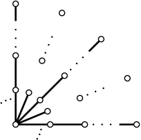
Figure 4. The ascending link of $v$.

The handle additions. For integers $a<b$ we obtain $f^{-1}([a,b])$ from $f^{-1}([a+1,b])$ by a succession of three types of coning operations (equivalently, handle addition operations).

1. For each $0$-cell $v\in f^{-1}(a)$, let $U_{v}$ denote the union of all the cells of $X$, each of which contains $v$ and which maps to the interval $[a,a+1]$ under $f$. Then $U_{v}\cap f^{-1}(a+1)$ is a geometric realization of $Lk_{\uparrow}(v,X)$.

   Attaching the $U_{v}$ to $f^{-1}([a+1,b])$ for each $0$-cell $v\in f^{-1}(a)$ is equivalent to coning off each $U_{v}\cap f^{-1}(a+1)$ copy of $Lk_{\uparrow}(v,X)$ to the corresponding vertex $v$. Denote the resulting complex by $X_{1}$.

   Now $Lk_{\uparrow}(v,X)$ has $(13m+1)$-components, each of which are contractible. Thus coning the copy of $Lk_{\uparrow}(v,X)$ in $f^{-1}(a+1)$ off to $v$ is equivalent to attaching a wedge of $13m$ one-handles to $f^{-1}([a+1,b])$. Thus $X_{1}$ is obtained from $f^{-1}([a+1,b])$ by attaching an infinite family of distinct wedges of $13m$ one-handles, indexed by the $0$-cells of $f^{-1}(a)$.

2. For each $1$-cell $e$ in $f^{-1}(a)$, let $U_{e}$ denote the union of cells, each of which contains $e$ and which maps to $[a,a+1]$ under $f$. Then $U_{e}\cap f^{-1}(a+1)$ is a geometric realization of $Lk_{\uparrow}(e,X)$. This is a discrete set of points. We see that its cardinality is at least one, by writing $e=a_{i}$ for some $1\leq i\leq m$, and noting that $Lk(a_{i},\Gamma_{i})$ is a subset of $Lk_{\uparrow}(e,X)$. Recall that $\Gamma_{i}$ is the simplex containing the bottom edge $a_{i}$ in the subdivision of $t^{-1}a_{i}tV_{i}^{-1}$ in Figure 3.

   Note also that $U_{e}\cap X_{1}$ is isomorphic to $Lk_{\uparrow}(e,X)\ast\partial e$. Thus, attaching $U_{e}$ to $X_{1}$ is equivalent to coning $Lk_{\uparrow}(e,X)\ast\partial e$ off to the barycenter $\widehat{e}$ of $e$. Since $\partial e$ has two points, this is equivalent to attaching a wedge of $(|Lk_{\uparrow}(e,X)|-1)$ two-handles to $X_{1}$. This even makes sense in the case that $Lk_{\uparrow}(e,X)$ has only one point. Then the coning operation is a homotopy equivalence, which is equivalent to attaching 0 two-handles to $X_{1}$.

   Let $X_{2}$ denote the result of attaching $U_{e}$ to $X_{1}$ for each $2$-cell $e$ in $f^{-1}(a)$. As in the previous section, $X_{2}$ is obtained from $X_{1}$ by attaching an infinite family of wedges of two-handles to $X_{1}$, indexed by $1$-cells $e$ in $f^{-1}(a)$.

3. Finally, attach the $2$-cells $d\subset f^{-1}(a)$ to $X_{2}$ to obtain $f^{-1}([a,b])$. Note that $d\cap X_{2}=\partial d$ for each such $2$-cell, and so attaching $d$ is equivalent to coning off $\partial d$ to the barycenter $\widehat{d}$ of $d$.

The handle cancellations. We show that a subset (described in Definition 3.4 below) of the two-handles from the coning operation (2) above cancel with the collection of all one-handles from the coning operation (1). Note that $X_{1}$ is the result of attaching all the one-handles to $f^{-1}([a+1,b])$. By cancel we simply mean that the space obtained from $X_{1}$ by attaching this subset of two-handles is homotopy equivalent to $f^{-1}([a+1,b])$.

Definition 3.4 (Canceling set).

For each $1\leq\ell\leq m$ and for each horizontal edge $a_{\ell}\subset f^{-1}(a)$, consider the union $U_{a_{\ell}}$ of $2$-cells of $X$, each of which contains $a_{\ell}$ and which maps to $[a,a+1]$ under $f$. Let $U^{\prime}_{a_{\ell}}$ denote the subcomplex of $U_{a_{\ell}}$ such that $Lk(a_{\ell},U^{\prime}_{a_{\ell}})$ is isomorphic to

$$Lk(a_{\ell},\Gamma_{\ell})\;\cup\;\bigcup_{\sigma_{i}(j)=\ell,\,j\not=1}Lk(a_{\sigma_{i}(j)},\Delta_{i,j}).$$

That is, we are not considering contributions to $Lk_{\uparrow}(a_{\ell},X)$ which correspond to occurrences of $a_{\ell}$ as the first letter in any $W_{i}$. The canceling set is defined as the following subcomplex of $f^{-1}([a,a+1])$

$$U\;=\;\bigcup_{1\leq\ell\leq m,\,a_{\ell}\subset f^{-1}(a)}U^{\prime}_{a_{\ell}}.$$

The shaded portion of Figure 5 shows the intersection of a $2$-cell $ta_{i}t^{-1}W_{i}^{-1}$ in $f^{-1}([a,a+1])$ with $X_{1}\cup U$.

Lemma 3.5 (Handle cancelation for ascending links).

Let $f:X\to\mathbb{R}$ be as defined above. Given integers $a<b$, let $X_{1}$ be the space obtained from $f^{-1}([a+1,b])$ by attaching $1$-handles as described in coning operation (1) above, and let $U$ be the canceling set of Definition 3.4.

Then $X_{1}\cup U$ is homotopy equivalent to $f^{-1}([a+1,b])$.

Proof.

The homotopy equivalence is fairly easy to see. First, consider relator cells of the form $ta_{i}t^{-1}W_{i}^{-1}\subset f^{-1}([a,a+1])$. Figure 5 shows the intersection of $X_{1}\cup U$ with one of these relators. The only cell of this relator which does not belong to $X_{1}\cup U$ is the unshaded (open) $2$-cell labeled $\Delta_{i,1}$. There is an obvious deformation retraction of this intersection onto the boundary $1$-skeleton $ta_{i}t^{-1}W_{i}^{-1}$. Perform all these deformation retractions for each $a_{i}\subset f^{-1}(a+1)$ and each $1\leq i\leq m$, to get the space $Z$.

\psfrag{ai}{$a_{i}$}\psfrag{as1}{$a_{\sigma_{i}(1)}$}\psfrag{as2}{$a_{\sigma_{i}(2)}$}\psfrag{as3}{$a_{\sigma_{i}(3)}$}\psfrag{as14}{$a_{\sigma_{i}(14)}$}\psfrag{t}{$t$}\psfrag{c}{$\cdots$}\includegraphics{retraction.eps}

Figure 5. Step one of the deformation retraction in Lemma 3.5.

Now, we turn our focus to horizontal $1$-cells at height $a$ in the set $Z$. Each $a_{j}\subset f^{-1}(a)$ is contained in just one $2$-cell of $Z$. This $2$-cell is labeled $\Gamma_{j}$. Push across the free edge $a_{j}$ to deformation retract the relator $t^{-1}V_{j}ta_{j}^{-1}$ onto the subword $t^{-1}V_{j}t$ of its boundary word. Do this equivariantly for all $1\leq j\leq m$ and all $a_{j}\subset f^{-1}(a)$. The resulting space can now be deformed to $f^{-1}([a+1,b])$ by collapsing the edges labeled $t$ in $f^{-1}([a,a+1])$ onto their vertices at level $a+1$. ∎

Continue with the usual Morse argument. We obtain $f^{-1}([a,b])$ from $f^{-1}([a+1,b])$ by first attaching all the new cells of $X_{1}\cup U$. Lemma 3.5 ensures that $X_{1}\cup U$ is homotopy equivalent to $f^{-1}([a+1,b])$. Now we obtain $f^{-1}([a,b])$ from $X_{1}\cup U$ by attaching all $2$-cells of $f^{-1}([a,a+1])$ which are labeled by $\Delta_{i,1}$ for $1\leq i\leq m$, and by attaching all $2$-cells of $f^{-1}(a)$. The boundary of each of these $2$-cells is contained in $X_{1}\cup U$, and so each such attachment can be viewed as a $2$-handle attachment (coning boundary off to barycenter).

In a similar fashion (working with descending links) one can argue that $f^{-1}([a,b+1])$ is obtained from $f^{-1}([a,b])$ up to homotopy by only attaching $2$-handles.

Now, the usual Morse theory arguments of [1] apply to conclude that the level set $f^{-1}(0)$ is connected, and hence that $K$ is finitely generated. Since we are attaching two-handles, the inclusion-induced map $H_{1}(f^{-1}([-n,n]))\to H_{1}(f^{-1}([-m,m]))$ for any integers $0<n<m$ is always a surjection. If this inclusion-induced homomorphism were ever the zero homomorphism, then we would have $H_{1}(f^{-1}([-m,m]))=0$. The two-handles attached to obtain $f^{-1}([-m-1,m+1])$ would produce nontrivial $2$-cycles in $f^{-1}([-m-1,m+1])\subset X$ which contradicts the fact that $X$ is a contractible $2$-complex. Now Theorem 2.2 of [6] (taking $\alpha\in{\mathbb{N}}$ and taking $X_{\alpha}$ to be $f^{-1}([-\alpha,\alpha])$) implies that $K$ is not FP₂. In particular, $K$ is not finitely presented. ∎

4. Conjugacy classes in finitely presented subgroups of hyperbolic groups

In this section we construct a hyperbolic group with a finitely presented subgroup which has infinitely many conjugacy classes of finite-order elements. Our construction is a modification of the construction in [2] of a hyperbolic group with a finitely presented subgroup which is not hyperbolic. The hyperbolic group in [2] is torsion-free, and does not admit any obvious finite-order automorphisms.

Theorem 4.1.

There exist hyperbolic groups containing finitely presented subgroups which have infinitely many conjugacy classes of finite order elements.

As indicated above, the proof consists in constructing a variation of the branched cover complex in [2]. The variation will have an added symmetry that the construction in [2] lacked. This symmetry will enable one to extend the groups under consideration by a finite-order automorphism, and to apply Proposition 1.1. An overview of the branched cover which parallels the construction in [2] is provided in subsection 4.1 below, and the proof that this branched cover does indeed admit a symmetry is given in subsection 4.2.

4.1. The branched cover $Y$

Let $\Theta$ be the graph in Figure 6, where each edge is isometric to the unit interval. Then $\Theta^{3}$, with the product metric, is a piecewise Euclidean cubical complex of non-positive curvature. The hyperbolic group in [2] is defined to be the fundamental group of a particular branched cover $Y$ of $\Theta^{3}$ with branching locus

$$L\;=\;(\Theta\times\{0\}\times\{1\})\;\cup\;(\{1\}\times\Theta\times\{0\})\;\cup\;(\{0\}\times\{1\}\times\Theta)\,.$$

\psfrag{0}{$0$}\psfrag{1}{$1$}\psfrag{a}{$a$}\psfrag{b}{$b$}\psfrag{c}{$c$}\psfrag{d}{$d$}\includegraphics[width=170.71652pt]{theta.eps}

Figure 6. The graph $\Theta$.

We refer to Section 5 of [2] for background on branched covers. Recall from [2] that the branched cover $Y$ is obtained by the following procedure.

• Remove the branching locus $L$ from the non-positively curved cubed complex $\Theta^{3}$. The resulting space $\Theta^{3}-L$ has an incomplete piecewise Euclidean metric.

• Take a finite cover of $\Theta^{3}-L$. The piecewise Euclidean metric on $\Theta^{3}-L$ lifts to an incomplete piecewise Euclidean metric on this cover.

• Complete this metric to form the branched cover $Y\to\Theta^{3}$.

In Lemma 5.5 of [2] it is shown that if $X$ is a non-positively curved piecewise Euclidean cubical complex and if $L\subset X$ is any reasonable branching locus, then every finite branched cover of $X$ over $L$ is itself a non-positively curved piecewise Euclidean cubical complex. In particular, every finite branched cover $Y$ of $\Theta^{3}$ over $L$ above is a non-positively curved piecewise Euclidean cubical complex.

Now we define a Morse function on $\Theta^{3}$, and hence on finite branched covers $Y$ of $\Theta^{3}$. There is a map $\Theta\to S^{1}$ which maps the vertices $0$ and $1$ to a base vertex of $S^{1}$, and maps the edges isometrically around the circle, with orientations specified by the arrows in Figure 6. This defines a map $\Theta^{3}\to S^{1}\times S^{1}\times S^{1}$. Composition with the standard linear map $S^{1}\times S^{1}\times S^{1}\to S^{1}$ (the one covered by $\mathbb{R}^{3}\to\mathbb{R}:(x,y,z)\mapsto x+y+z$) gives a map $\Theta^{3}\to S^{1}$. Finally, the composition $Y\to\Theta^{3}\to S^{1}$ is a circle-valued Morse function on the branched cover $Y$.

The majority of the work in [2] comes from constructing a specific finite branched cover $Y$ having the following properties.

Hyperbolic:

$\pi_{1}(Y)$ is a hyperbolic group, and

F₂–not–F₃:

the kernel of the map $\pi_{1}(Y)\to\pi_{1}(S^{1})$ is finitely presented, but not of type F₃.

These properties are guaranteed by items (3) and (4) of Theorem 6.1 of [2]. The construction of the branched cover $Y$ is described in detail in the proof of Theorem 6.1. We sketch the main points below, and indicate our variation on that construction. The key point is that our variation is equivariant with respect to a particular isometry $\sigma\colon\thinspace\Theta\to\Theta$ (see Section 4.2) and so the branched cover $Y$ admits an isometry $\eta$ induced by $\sigma$.

1. For each $1\leq i\leq 3$ there are projection maps

   $${\rm pr}_{i}\colon\thinspace\Theta^{3}\;\to\;\Theta^{2}:(x_{1},x_{2},x_{3})\;\mapsto\;(x_{i+1},x_{i+2})$$

   where $i$ is taken modulo $3$, and we use $3$ in place of $0$.

   These restrict to projection maps

   $${\rm pr}_{i}\colon\thinspace\Theta^{3}-L\;\to\;\Theta^{2}-\{(0,1)\}$$

   for $1\leq i\leq 3$.

2. Let $\Delta$ be the graph (depicted in Figure 7)

   $$\Theta\times\{0\}\;\cup\;\{1\}\times\Theta\subset\Theta^{2}-\{(0,1)\}.$$

   \psfrag{(0,0)}{{\scriptsize$(0,0)$}}\psfrag{(1,0)}{{\scriptsize$(1,0)$}}\psfrag{(1,1)}{{\scriptsize$(1,1)$}}\psfrag{a0}{$a_{0}$}\psfrag{b0}{$b_{0}$}\psfrag{c0}{$c_{0}$}\psfrag{d0}{$d_{0}$}\psfrag{a1}{$a_{1}$}\psfrag{b1}{$b_{1}$}\psfrag{c1}{$c_{1}$}\psfrag{d1}{$d_{1}$}\includegraphics[width=327.20668pt]{delta.eps}

   Figure 7. The graph $\Delta$.

   By Lemma 6.2 of [2], the inclusion of $\Delta$ in $\Theta^{2}-\{(0,1)\}$ is a homotopy equivalence. We choose the following basis for $\pi_{1}(\Delta,(1,0))$, which is a free group of rank $6$:

   $$\bar{a}_{0}b_{0},\;\bar{a}_{0}\bar{c}_{0},\;\bar{a}_{0}\bar{d}_{0},\;a_{1}\bar{b}_{1},\;a_{1}c_{1},\;a_{1}d_{1}$$

3. Define a homomorphism $\rho\colon\thinspace\pi_{1}(\Delta,(0,1))\to S_{5}$ (when convenient, we shall think of $\rho$ as a homomorphism $\rho\colon\thinspace\pi_{1}(\Theta^{2}-\{(0,0)\},(0,1))\to S_{5}$) by

   $$\bar{a}_{0}b_{0} \mapsto\alpha^{2} a_{1}\bar{b}_{1} \mapsto\beta^{2}$$

   $$\bar{a}_{0}\bar{c}_{0} \mapsto\alpha^{3} a_{1}c_{1} \mapsto\beta^{3}$$

   $$\bar{a}_{0}\bar{d}_{0} \mapsto\alpha a_{1}d_{1} \mapsto\beta$$

   where $\alpha$ and $\beta$ are the permutations

   $$\alpha=(1)(2\;5\;3\;4)\quad\text{and}\quad\beta=(1\;2\;3\;4)(5).$$

   The reader can verify that $[\alpha^{i},\beta^{j}]$ is a $5$-cycle for $1\leq i,j\leq 3$. This implies that the images under $\rho$ of the 36 commutators obtained by taking a pair of loops in $\Delta$ (one composed of two $1$-cells with endpoints $(0,0)$ and $(1,0)$, and the second composed of two $1$-cells with endpoints $(1,0)$ and $(1,1)$) are all $5$-cycles.

   Thus the homomorphism $\rho$ satisfies Property 1 in the proof of Theorem 6.1 of [2]. See Remark 4.2.

4. For $1\leq i\leq 3$ define homomorphisms $\rho_{i}\colon\thinspace\pi_{1}(\Theta^{3}-L,(0,0,0))\to S_{5}$ by

   $$\rho_{i}=\rho\circ\iota\circ{\rm{pr}}_{i}$$

   where $\iota\colon\thinspace\pi_{1}(\Theta^{2}-\{(0,0)\},(0,0))\to\pi_{1}(\Theta^{2}-\{(0,0)\},(1,0))$ is a change of basepoint isomorphism. Specifically, $\iota$ is the isomorphism induced by conjugating an edge path in $\Delta$ based at $(0,0)$ by the edge $\bar{a}_{0}$. For each $i$, this gives an action of $\pi_{1}(\Theta^{3}-L,(0,0,0))$ on the set $S=\{1,2,3,4,5\}$. Define an action of $\pi_{1}(\Theta^{3}-L,(0,0,0))$ on the set $S\times S\times S$ via

   $$\tau=(\rho_{1},\rho_{2},\rho_{3})\colon\thinspace\pi_{1}(\Theta^{3}-L,(0,0,0))\to S_{125}.$$

   The $125$-fold cover of $\Theta^{3}-L$ associated to $\tau$ is connected. Lift the local metric from $\Theta^{3}-L$ to $Y$, and complete it to obtain the branched covering $b\colon\thinspace Y\to\Theta^{3}$.

Remark 4.2.

Our version of $\rho$ satisfies the key Property 1 of Theorem 6.1 of [2]. Thus items (3) and (4) of Theorem 6.1 hold, and so the branched covering $Y$ will satisfy properties Hyperbolic and F₂–not–F₃ above.

However, our choice of $\rho$ has an extra symmetry built in that the one in [2] lacked. This symmetry will be crucial in Section 4.2 below.

4.2. The isometry $\eta\colon\thinspace Y\to Y$

Let $\sigma\colon\thinspace\Theta\to\Theta$ denote the isometry which fixes vertices $0$ and $1$ and transposes the edges $a$ and $b$, and the edges $c$ and $d$. This induces coordinate-wise defined isometries

$$\sigma_{2}\colon\thinspace\Theta^{2}\;\to\;\Theta^{2}\;:(x,y)\;\mapsto\;(\sigma(x),\sigma(y))$$

and

$$\sigma_{3}\colon\thinspace\Theta^{3}\;\to\;\Theta^{3}\;:(x,y,z)\;\mapsto\;(\sigma(x),\sigma(y),\sigma(z))\,.$$

These restrict to isometries of the incomplete spaces $\sigma_{2}\colon\thinspace\Theta^{2}-\{(0,1)\}\;\to\;\Theta^{2}-\{(0,1)\}$ and $\sigma_{3}\colon\thinspace\Theta^{3}-L\;\to\;\Theta^{3}-L$.

Then $\sigma_{2}\colon\thinspace\Theta^{2}-\{(0,1)\}\;\to\;\Theta^{2}-\{(0,1)\}$ induces a map $\sigma_{2}\colon\thinspace\Delta\to\Delta$. The action of $\sigma_{2}$ on $\Delta$ is given by $a_{i}\leftrightarrow b_{i}$, $c_{i}\leftrightarrow d_{i}$, $i=0,1$. Moreover, for $1\leq i\leq 3$, we have

$${\rm pr}_{i\ast}\circ\sigma_{3\ast}=\sigma_{2\ast}\circ{\rm pr}_{i\ast}.$$ (3)

Let $C_{\alpha}\colon\thinspace S_{5}\to S_{5}$ be the inner automorphism $x\mapsto\alpha x\alpha^{-1}$.
Claim. The following two maps $\pi_{1}(\Theta^{2}-\{(1,0)\},(0,0))\to S_{5}$ are equal:

$$\rho\circ\iota\circ\sigma_{2\ast}=C_{\alpha}^{2}\circ\rho\circ\iota$$ (4)

Indeed, using the fact that $\alpha,\beta$ are $4$-cycles, we can check equality on a free basis as follows:

$$\rho\iota\sigma_{2\ast}(b_{0}\bar{a}_{0}) =\rho\iota(a_{0}\bar{b}_{0})=\rho(\bar{b}_{0}a_{0})=\alpha^{-2}$$

$$=\alpha^{2}=C_{\alpha}^{2}\rho(\bar{a}_{0}b_{0})=C_{\alpha}^{2}\rho\iota(b_{0}\bar{a}_{0})$$

$$\rho\iota\sigma_{2\ast}(\bar{c}_{0}\bar{a}_{0}) =\rho\iota(\bar{d}_{0}\bar{b}_{0})=\rho(\bar{a}_{0}\bar{d}_{0}\bar{b}_{0}a_{0})=\alpha^{-1}$$

$$=\alpha^{3}=C_{\alpha}^{2}\rho(\bar{a}_{0}\bar{c}_{0})=C_{\alpha}^{2}\rho\iota(\bar{c}_{0}\bar{a}_{0})$$

$$\rho\iota\sigma_{2\ast}(\bar{d}_{0}\bar{a}_{0}) =\rho\iota(\bar{c}_{0}\bar{b}_{0})=\rho(\bar{a}_{0}\bar{c}_{0}\bar{b}_{0}a_{0})=\alpha$$

$$=C_{\alpha}^{2}\rho(\bar{a}_{0}\bar{d}_{0})=C_{\alpha}^{2}\rho\iota(\bar{d}_{0}\bar{a}_{0})$$

$$\rho\iota\sigma_{2\ast}(a_{0}a_{1}\bar{b}_{1}\bar{a}_{0}) =\rho\iota(b_{0}b_{1}\bar{a}_{1}\bar{b}_{0})=\rho(\bar{a}_{0}b_{0}b_{1}\bar{a}_{1}\bar{b}_{0}a_{0})=\alpha^{2}\beta^{-2}\alpha^{-2}$$

$$=\alpha^{2}\beta^{2}\alpha^{-2}=C_{\alpha}^{2}\rho(a_{1}\bar{b}_{1})=C_{\alpha}^{2}\rho\iota(a_{0}a_{1}\bar{b}_{1}\bar{a}_{0})$$

$$\rho\iota\sigma_{2\ast}(a_{0}a_{1}c_{1}\bar{a}_{0}) =\rho\iota(b_{0}b_{1}d_{1}\bar{b}_{0})=\rho(\bar{a}_{0}b_{0}b_{1}d_{1}\bar{b}_{0}a_{0})=\alpha^{2}\beta^{-1}\alpha^{-2}$$

$$=\alpha^{2}\beta^{3}\alpha^{-2}=C_{\alpha}^{2}\rho(a_{1}c_{1})=C_{\alpha}^{2}\rho\iota(a_{0}a_{1}c_{1}\bar{a}_{0})$$

$$\rho\iota\sigma_{2\ast}(a_{0}a_{1}d_{1}\bar{a}_{0}) =\rho\iota(b_{0}b_{1}c_{1}\bar{b}_{0})=\rho(\bar{a}_{0}b_{0}b_{1}c_{1}\bar{b}_{0}a_{0})=\alpha^{2}\beta\alpha^{-2}$$

$$=C_{\alpha}^{2}\rho(a_{1}d_{1})=C_{\alpha}^{2}\rho\iota(a_{0}a_{1}d_{1}\bar{a}_{0})$$

and so the claim is established.

The symmetry in equation (4) is key to showing that $\sigma_{3}$ lifts to an automorphism $\eta$ of $Y$. First, equation (4) is used to show that $\sigma_{3}\colon\thinspace\Theta^{3}-L\to\Theta^{3}-L$ lifts to a symmetry of the $125$-fold cover, and then the isometry $\eta$ is obtained by continuous extension to the completion $Y$ of this cover.

Recall from item (iv) of subsection 4.1 that the $125$-fold cover of $\Theta^{3}-L$ corresponds to the subgroup

$$H\;=\;\tau^{-1}({\rm Stab}_{S_{125}}((1,1,1)))$$

of $\pi_{1}(\Theta^{3}-L,(0,0,0))$. By construction, $H=H_{1}\cap H_{2}\cap H_{3}$, where

$$H_{i}=\rho_{i}^{-1}(\rm{Stab}_{S_{5}}(1)),\qquad\text{for}\;\;1\leq i\leq 3.$$

The isometry $\sigma_{3}$ lifts to this cover provided that $\sigma_{3\ast}(H)\subset H$. This will follow if $\sigma_{3\ast}(H_{i})\subset H_{i}$ for $1\leq i\leq 3$. If $h\in H_{i}$, (i.e. $\rho_{i}(h)\in\rm{Stab}_{S_{5}}(1)$) then

$$\rho_{i}\sigma_{3\ast}(h)(1) =\rho\iota{\rm pr}_{i\ast}\sigma_{3\ast}(h)(1) \rho_{i}$$ definition of

$$=\rho\iota\sigma_{2\ast}{\rm{pr}}_{i\ast}(h)(1)$$

$$=C_{\alpha}^{2}\rho\iota{\rm{pr}}_{i\ast}(h)(1)$$ equation (4)

$$=C_{\alpha}^{2}\rho_{i}(h)(1) \rho_{i}$$ definition of

$$=\alpha^{2}\rho_{i}(h)\alpha^{-2}(1) C_{\alpha}$$ definition of

$$=1 \rho_{i}(h),\alpha\in\rm{Stab}_{S_{5}}(1)$$ as

We have shown $\rho_{i}(\sigma_{3\ast}(h))\in{\rm Stab}_{S_{5}}(1)$. Thus $\sigma_{3\ast}(H_{i})\subset H_{i}$, and so $\sigma_{3}$ lifts to the $125$-fold cover of $\Theta^{3}-L$.

Since $\sigma_{3}$ fixes the vertex $(0,0,0)\in\Theta^{3}-L$ and acts freely on the link of $(0,0,0)$, we can choose a lift $\widehat{\sigma}_{3}$ to the $125$-fold cover which fixes a vertex $v$ in the fiber over $(0,0,0)$, and acts freely on the link of this vertex. Thus the continuous extension $\eta\colon\thinspace Y\to Y$ of $\widehat{\sigma}_{3}$ is an isometry which fixes a vertex of $b^{-1}((0,0,0))\subset Y$, and which acts freely on the link of this vertex.

The square $\widehat{\sigma}_{3}^{2}$ also fixes $v$ and, covers the identity map $\sigma_{3}^{2}\colon\thinspace\Theta^{3}-L\to\Theta^{3}-L$. Thus $\widehat{\sigma}_{3}^{2}$ is a deck transformation of the $125$-fold cover of $\Theta^{3}-L$ which fixes a point, and so is the identity map. Its continuous extension $\eta^{2}$ is the identity map on $Y$, and so $\eta$ is an order two isometry of $Y$.

Let $K$ be the kernel of the map $\pi_{1}(Y)\to\pi_{1}(S^{1})$. By Remark 4.2 $\pi_{1}(Y)$ is hyperbolic, and $K$ is finitely presented but not of type F₃. Since $\eta$ has finite order, the subgroup $K\rtimes\langle\eta\rangle\subset\pi_{1}(Y)\rtimes\langle\eta\rangle$ is a finitely presented subgroup of the hyperbolic group $\pi_{1}(Y)\rtimes\langle\eta\rangle$ which has infinitely many conjugacy classes of finite-order elements. The conjugacy class count follows either from Proposition 1.1 above, or from Proposition 1.1 of [3].

References

[1]M. Bestvina and N. Brady, Morse theory and finiteness properties of
groups, Invent. Math., 129 (1997), pp. 445–470.
[2]N. Brady, Branched coverings of cubical complexes and subgroups of
hyperbolic groups, J. London Math. Soc. (2), 60 (1999), pp. 461–480.
[3]N. Brady, M. Clay, and P. Dani, Morse theory and conjugacy classes
of finite subgroups, Geom. Dedicata, 135 (2008), pp. 15–22.
[4]N. Brady and A. Miller, structures for free-by-free
groups, Geom. Dedicata, 90 (2002), pp. 77–98.
[5]M. R. Bridson, Finiteness properties for subgroups of , Math. Ann., 317 (2000), pp. 629–633.
[6]K. S. Brown, Finiteness properties of groups, in Proceedings of the
Northwestern conference on cohomology of groups (Evanston, Ill., 1985),
vol. 44, 1987, pp. 45–75.
[7]M. Feighn and G. Mess, Conjugacy classes of finite subgroups of
Kleinian groups, Amer. J. Math., 113 (1991), pp. 179–188.
[8]I. J. Leary and B. E. A. Nucinkis, Some groups of type ,
Invent. Math., 151 (2003), pp. 135–165.
[9]D. T. Wise, Incoherent negatively curved groups, Proc. Amer. Math.
Soc., 126 (1998), pp. 957–964.