The DSUB$m$ Approximation Scheme for the Coupled Cluster Method and Applications to Quantum Magnets

Abstract

A new approximate scheme, DSUB$m$, is described for the coupled cluster method. We then apply it to two well-studied (spin-1/2 Heisenberg antiferromagnet) spin-lattice models, namely: the $XXZ$ and the $XY$ models on the square lattice in two dimensions. Results are obtained in each case for the ground-state energy, the sublattice magnetization and the quantum critical point. They are in good agreement with those from such alternative methods as spin-wave theory, series expansions, quantum Monte Carlo methods and those from the CCM using the LSUB$m$ scheme.

Key words: Coupled cluster method; quantum antiferromagnet

PACS: 75.10.Jm, 75.30.Gw, 75.40.-s, 75.50.Ee

1 Introduction

The coupled cluster method (CCM) is a universal microscopic technique of quantum many-body theory [1, 2, 3, 4, 5, 6, 7, 8, 9]. It has been applied successfully to many physical systems including:

• systems existing in the spatial continuum, e.g., the electron gas [10, 11], atomic nuclei and nuclear matter [12, 13], and molecules [14]; and

• systems on a discrete spatial lattice, e.g., spin-lattice models of quantum magnetism [15, 16, 17, 18, 19, 20, 21, 22, 23, 24, 25, 26, 27].

A special characteristic of the CCM is that it deals with infinite systems from the outset, and hence one never needs to take the limit $N\rightarrow\infty$ explicitly in the number, $N$, of interacting particles or the number of sites in the lattice. However, approximations in the inherent cluster expansions for the correlation operators are required. Several efficient and systematic approximation schemes for the CCM have been specifically developed by us previously for use with lattice systems [16, 28, 29, 30]. Up till now the most favoured and most successful CCM approximation schemes for lattices have been the so-called LSUB$m$ and SUB$n$–$m$ schemes that we describe more fully below in section 3. Although the LSUB$m$ scheme, in particular, has been shown to be highly successful in practice for a wide variety of both frustrated and unfrustrated spin-lattice systems, a disadvantage of this scheme is that the number of spin configurations generally rises very rapidly with the truncation index $m$. This motivates us to develop alternative schemes which satisfy one or both of the following two criteria:

• that we are able to calculate more levels of approximation within the scheme, and hence have available more data points for the necessary extrapolations for calculated physical quantities to the exact limit where all configurations are retained; and

• that one can capture the physically most important configurations at relatively low orders, so that the quantities of interest converge more rapidly with the truncation index.

A main aim of our work is thus to provide users of the CCM with more choices of approximation scheme. In this paper we outline the formal aspects, of and present preliminary results for some benchmark models for, a new CCM approximation scheme, called the DSUB$m$ scheme, for use with systems described on a spatial lattice. The rest of the paper is organized as follows. In section 2 we introduce the CCM formalism in general. In section 3 we then discuss the specific application of the CCM to spin-lattice systems. We consider in section 4 both the existing truncation schemes and introduce the alternative new DSUB$m$ scheme. In order to evaluate the accuracy of the new approximation scheme we apply it to two very well-studied antiferromagnetic spin-lattice models [18, 20], namely: the $XXZ$ and the $XY$ models on the square lattice in two dimensions (2D). Both models have a quantum phase transition. They have also been very successfully investigated by the CCM within the LSUB$m$ scheme for the ground-state (gs) energy and the gs order parameter which is, in our case, the sublattice magnetization. All techniques applied to lattice spin systems need to be extrapolated in terms of some appropriate parameters. For exact diagonalization and quantum Monte Carlo methods, this is the lattice size $N$. As noted above, one good aspect of the CCM is that we may work in the limit of infinite lattice size ($N\rightarrow\infty$) from the outset. By contrast, the extrapolation for the CCM is in terms of some truncation index $m$, where in the limit $m\rightarrow\infty$ we retain all configurations. The CCM extrapolations that have been used up till now in the trunction index, e.g., $m$ for the LSUB$m$ approximation, are heuristic schemes, but we have considerable prior experience [20, 29, 31, 32, 33] in using and refining them, as described in section 5. The new DSUB$m$ approximation scheme is then applied to the square-lattice spin-$1/2$ antiferromagnetic $XXZ$ model in section 6 and the corresondingly $XY$ model in section 7, respectively. The results for both models are compared critically with those from the corresponding LSUB$m$ scheme and also with the results from other methods. Finally, our conclusions are given in section 8 where we reiterate a brief summary of the results.

2 The CCM Formalism

This section briefly describes the CCM formalism (and see e.g., Refs. [8, 9] for further details). A first step in any CCM application is to choose a normzalized model (or reference) state $|\Phi\rangle$ that can act as a cyclic vector with respect to a complete set of mutually commuting multiconfigurational creation operators $C^{+}_{I}\equiv(C^{-}_{I})^{\dagger}$. The index $I$ here is a set-index that labels the many-particle configuration created in the state $C^{+}_{I}|\Phi\rangle$. The exact ket and bra gs energy eigenstates $|\Psi\rangle$ and $\langle\tilde{\Psi}|$, of the many-body system are then parametrised in the CCM form as:                                       Ket-state   Bra-state

$$|\Psi\rangle=\mbox{e}^{S}|\Phi\rangle\,;\qquad\langle\tilde{\Psi}|=\langle\Phi|\tilde{S}\mbox{e}^{-S}\,,$$ (1)

$$S=\sum_{I\neq 0}{\cal S}_{I}C^{+}_{I}\,;\qquad\tilde{S}=1+\sum_{I\neq 0}\tilde{{\cal S}_{I}}C^{-}_{I}\,,$$ (2)

$$H|\Psi\rangle=E|\Psi\rangle\,;\qquad\langle\tilde{\Psi}|H=E\langle\tilde{\Psi}|\,,$$ (3)

where we have defined $C^{+}_{0}\equiv 1\equiv C^{-}_{0}$. The requirements on the multiconfigurational creation operators are that any many-particle state can be written exactly and uniquely as a linear combination of the states $\{C^{+}_{I}|\Phi\rangle\}$, which hence fulfill the completeness relation

$$\sum_{I}C^{+}_{I}|\Phi\rangle\langle\Phi|C^{-}_{I}=1=|\Phi\rangle\langle\Phi|+\sum_{I\neq 0}C^{+}_{I}|\Phi\rangle\langle\Phi|C^{-}_{I}\,,$$ (4)

together with the conditions,

$$C^{-}_{I}|\Phi\rangle=0=\langle\Phi|C^{+}_{I}\,;\qquad\forall\emph{I}\neq 0\,,$$ (5)

$$[C^{+}_{I},C^{+}_{J}]=0=[C^{-}_{I},C^{-}_{J}]\,.$$ (6)

Approximations are necessary in practice to restrict the label set I to some finite (e.g., LSUB$m$) or infinite (e.g., SUB$n$) subset, as described more fully below. The correlation operator $S$ is a linked-cluster operator and is decomposed in terms of a complete set of creation operators ${C^{+}_{I}}$. It creates excitations on the model state by acting on it to produce correlated cluster states. Although the manifest Hermiticity, $(\langle\tilde{\Psi}|)^{\dagger}\equiv|\Psi\rangle/\langle\Psi|\Psi\rangle$, is lost, the normalization conditions $\langle\tilde{\Psi}|\Psi\rangle=\langle\Phi|\Psi\rangle=\langle\Phi|\Phi\rangle\equiv 1$ are preserved. The CCM Schrödinger equations (3) are thus writtern as

$$H\mbox{e}^{S}|\Phi\rangle=E\mbox{e}^{S}|\Phi\rangle\,;\qquad\langle\Phi|\tilde{S}\mbox{e}^{-S}H=E\langle\Phi|\tilde{S}\mbox{e}^{-S}\,;$$ (7)

and its equivalent similarity-transformed form becomes

$$\mbox{e}^{-S}H\mbox{e}^{S}|\Phi\rangle=E|\Phi\rangle\,;\qquad\langle\Phi|\tilde{S}\mbox{e}^{-S}H\mbox{e}^{S}=E\langle\Phi|\tilde{S}\,.$$ (8)

We note that while the parametrizations of equations (1) and (2) are not manifestly Hermitian conjugate, they do preserve the important Hellmann-Feynman theorem at all levels of approximations (viz., when the complete set of many-particle configurations $I$ is truncated) [9]. Furthermore, the amplitudes (${\cal S}_{I},\tilde{\cal S}_{I}$) form canonically conjugate pairs in a time-dependent version of the CCM, by contrast with the pairs (${\cal S}_{I},{\cal S}^{\ast}_{I}$) coming from a manifestly Hermitian-conjugate representation for $\langle\tilde{\Psi}|=(\langle\Phi|\mbox{e}^{S^{\dagger}}\mbox{e}^{S}|\Phi\rangle)^{-1}\langle\Phi|\mbox{e}^{S^{\dagger}}$, which are not canonically conjugate to one another.

The static gs CCM correlation operators $S$ and $\tilde{S}$ contain the real $c$-number correlation coefficients ${\cal S}_{I}$ and ${\tilde{\cal S}}_{I}$ that need to be calculated. Clearly, once the coefficients $\{{\cal S}_{I},\tilde{\cal S}_{I}\}$ are known, all other gs properties of the many-body system can be derived from them. For example, the gs expectation value of an arbitrary operator $A$ can be expressed as

$$\bar{A}\equiv\langle A\rangle\equiv\langle\tilde{\Psi}|A|\Psi\rangle=\langle\Phi|\tilde{S}\mbox{e}^{-S}A\mbox{e}^{S}|\Phi\rangle\equiv A({\cal S}_{I},\tilde{{\cal S}_{I}})\,.$$ (9)

To find the gs correlation coefficients $\{{\cal S}_{I},\tilde{\cal S}_{I}\}$ we simply insert the parametrization of equation (2) into the Schrödinger equations (8), and project onto the complete sets of states $\{\langle\Phi|C^{-}_{I}\}$ and $\{C^{+}_{I}|\Phi\rangle\}$, respectively,

$$\langle\Phi|C^{-}_{I}\mbox{e}^{-S}H\mbox{e}^{S}|\Phi\rangle=0\,;\qquad\forall I\neq 0\,.$$ (10)

$$\langle\Phi|\tilde{S}(\mbox{e}^{-S}H\mbox{e}^{S}-E)C^{+}_{I}|\Phi\rangle=0\;;\hskip 14.45377pt\forall I\neq 0\,.$$ (11)

Equation (11) may also easily be rewritten, by pre-multiplying the ket-state equation (8) with the state $\langle\Phi|\tilde{S}C^{+}_{I}$ and using the commutation relation (6), in the form

$$\langle\Phi|\tilde{S}\mbox{e}^{-S}[H,C^{+}_{I}]\mbox{e}^{S}|\Phi\rangle=0\,;\qquad\forall I\neq 0\,.$$ (12)

Equations (10)–(12) may be equivalently derived by requiring that the gs energy expectation value, $\bar{H}\equiv\langle\tilde{\Psi}|H|\Psi\rangle=\langle\Phi|\tilde{S}\mbox{e}^{-S}H\mbox{e}^{S}|\Phi\rangle$, is minimized with respect to the entire set $\{{\cal S}_{I},{\tilde{\cal S}}_{I}\}$. In practice we thus need to solve equations (10) and (12) for the set $\{{\cal S}_{I},{\tilde{\cal S}}_{I}\}$. We note that equations (9) and (10) show that the gs energy at the stationary point has the simple form

$$E\equiv E({\cal S}_{I})=\langle\Phi|\mbox{e}^{-S}H\mbox{e}^{S}|\Phi\rangle\,,$$ (13)

which also follows immediately from the ket-state equation (8) by projecting it onto the state $\langle\Phi|$. It is important to note that this (bi-)variational formulation does not necessarily lead to an upper bound for $E$ when the summations over the index set $\{I\}$ for $S$ and $\tilde{S}$ in equation (2) are truncated, due to the lack of manifest Hermiticity when such approximations are made. Nevertheless, as we have pointed out above, one can prove [9] that the important Hellmann-Feynman theorem is preserved in all such approximations.

We note that equation (10) represents a coupled set of multinomial equations for the $c$-number correlation coefficients $\{{\cal S}_{I}\}$. The nested commutator expansion of the similarity-transformed Hamiltonian,

$$\mbox{e}^{-S}H\mbox{e}^{S}=H+[H,S]+\frac{1}{2!}[[H,S],S]+\cdots\,,$$ (14)

and the fact that all of the individual components of $S$ in the decomposition of equation (2) commute with one another by construction [and see equation (6)], together imply that each element of $S$ in equation (2) is linked directly to the Hamiltonian in each of the terms in equation (14). Thus, each of the coupled equations (10) is of Goldstone linked-cluster type. In turn this guarantees that all extensive variables, such as the energy, scale linearly with particle number $N$. Thus, at any level of approximation obtained by truncation in the summations on the index $I$ in the parametrizations of equation (2), we may (and, in practice, do) work from the outset in the limit $N\rightarrow\infty$ of an infinite system.

Furthermore, each of the seemingly infinite-order (in $S$) linked-cluster equations (10) will actually be of finite length when expanded using equation (14), since the otherwise infinite series of equation (14) will actually terminate at a finite order, provided only (as is usually the case, including those for the Hamiltonians considered in this paper) that each term in the Hamiltonian $H$ contains a finite number of single-particle destruction operators defined with respect to the reference (or generalized vacuum) state $|\Phi\rangle$. Hence, the CCM parametrization naturally leads to a workable scheme that can be implemented computationally in an efficient manner to evaluate the set of configuration coefficients $\{{\cal S}_{I},{\tilde{\cal S}}_{I}\}$ by solving the coupled sets of equations (10) and (12), once we have devised practical and systematic truncation hierarchies for limiting the set of multiconfigurational set-indices $\{I\}$ to some suitable finite or infinite subset.

3 CCM for Spin-Lattice Systems

We will discuss various practical CCM truncation schemes that fulfill the criteria of being systematically improvable in some suitable truncation index $m$, and that can be extrapolated accurately in practice to the exact, $m\rightarrow\infty$, limit for calculated physical quantities. Before doing so, however, we first describe how the general CCM formalism described in section 2 is implemented for spin-lattice problems in practice. As is the case for any application of the CCM to a general quantum many-body system, the first step is to choose a suitable reference state $|\Phi\rangle$ in which the the state of the spin (viz., in practice, its projection onto a specific quantization axis in spin space) on every lattice site $k$ is characterized. Clearly, the choice of $|\Phi\rangle$ will depend on both the system being studied and, more importantly, which of its possible phases is being considered. We describe examples of such choices later for the particular models that we utilize here as test cases for our new truncation scheme.

Whatever the choice of $|\Phi\rangle$ we note firstly that is very convenient, in order to set up as universal a methodology as possible, to treat the spins on every lattice site in an arbitrarily given model state $|\Phi\rangle$ as being equivalent. A suitably simple way of so doing is to introduce a different local quantization axis and a correspondingly different set of spin coordinates on each lattice site $k$, so that all spins, whatever their original orientation in $|\Phi\rangle$ in a global spin-coordinate system, align along the same direction (which, to be specific, we henceforth choose as the negative $z$ direction) in these local spin-coordinate frames. This can always be done in practice by defining a suitable rotation in spin space of the global spin coordinates at each lattice site $k$. Such rotations are canonical transformations that leave unchanged the fundamental spin commutation relations,

$$[s^{+}_{k},s^{-}_{k^{\prime}}]=2s^{z}_{k}\delta_{kk^{\prime}}\,;\qquad[s^{z}_{k},s^{\pm}_{k^{\prime}}]=\pm s^{\pm}_{k}\delta_{kk^{\prime}}\,,$$ (15)

$$s^{\pm}_{k}\equiv s^{x}_{k}\pm is^{y}_{k}\,,$$ (16)

among the usual SU(2) spin operators ($s^{x}_{k},s^{y}_{k},s^{z}_{k}$) on lattice site $k$. Each spin has a total spin quantum number, $s_{k}$, where ${\bf s}^{2}_{k}=s_{k}(s_{k}+1)$ is the SU(2) Casimir operator. For the models considered here, $s_{k}=s=1/2$, $\forall k$.

In the local spin frames defined above the configuration indices $I$ simply become a set of lattice site indices, $I\rightarrow(k_{1},k_{2},\cdots,k_{m}$). The corresponding generalized multiconfigurational creation operators $C^{+}_{I}$ thus become simple products of single spin-raising operators, $C^{+}_{I}\rightarrow s^{+}_{k_{1}}s^{+}_{k_{2}}\cdots s^{+}_{k_{m}}$, and, for example, the ket-state CCM correlation operator is expressed as

$$S=\sum_{m}\sum_{{k_{1}}{k_{2}}\cdots{k_{m}}}{\cal S}_{k_{1}k_{2}\cdots k_{m}}s^{+}_{k_{1}}s^{+}_{k_{2}}\cdots s^{+}_{k_{m}}\,,$$ (17)

and $\tilde{S}$ is similarly defined in terms of the spin-lowering operators $s^{-}_{k}$. Since the operator $S$ acts on the state $|\Phi\rangle$, in which all spins point along the negative $z$-axis in the local spin-coordinate frames, every lattice site $k_{i}$ in equation (17) can be repeated up to no more than 2$s$ times in each term where it is allowed, since a spin $s$ has only ($2s+1$) possible projections along the quantization axis.

In practice the allowed configurations are often further constrained by symmetries in the problem and by conservation laws. An example of the latter is provided by the $XXZ$ model considered below in section 6, for which we can easily show that the total $z$-component of spin, $s^{T}_{z}=\sum^{N}_{k=1}s^{z}_{k}$, in the original global spin coordinates, is a good quantum number since $[s^{z}_{T},H]=0$ in this case. Finally, for the quasiclassical magnetically ordered states that we calculate here for both models in sections 6 and 7, the order parameter is the sublattice magnetization, $M$, which is given within the local spin coordinates defined above as

$$M\equiv-\frac{1}{N}\langle\tilde{\Psi}|\sum_{k}^{N}s^{z}_{k}|\Psi\rangle=-\frac{1}{N}\sum_{k}^{N}\langle\Phi|\tilde{S}\mbox{e}^{-S}s^{z}_{k}\mbox{e}^{S}|\Phi\rangle\,.$$ (18)

After the local spin axes have been chosen, the model state thus has all spins pointing downwards (i.e., in the negative $z$-direction, where $z$ is the quantization axis),

$$|\Phi\rangle=\bigotimes^{N}_{k_{1}}|\downarrow\rangle_{k}\,;\qquad\mbox{in the local spin axes,}$$ (19)

where $|\downarrow\rangle\equiv|s,-s\rangle$ in the usual $|s,m_{s}\rangle$ notation for single spin states.

The similarity-transformed Hamiltonian $\bar{H}\equiv\mbox{e}^{-S}H\mbox{e}^{-S}$, and all of the corresponding matrix elements in equations (9)–(13) and equation (18), for example, may then be evaluated in the local spin coordinate frames by using the nested commutator expansion of equation (14), the commutator relations of equation (15), and the simple universal relations

$$s^{-}_{k}|\Phi\rangle=0\,;\qquad\forall k\,,$$ (20)

$$s^{z}_{k}|\Phi\rangle\,;\qquad\forall k\,,$$ (21)

that hold at all lattice sites in the local spin frames.

4 Approximation schemes

The CCM formalism is exact if all many-body configurations $I$ are included in the $S$ and $\tilde{S}$ operators. In practice, it is necessary to use approximation schemes to truncate the correlation operators.

4.1 Common previous truncation schemes

The main approximation scheme used to date for continuous systems is the so-called SUB$n$ scheme described below. For systems defined on a regular periodic spatial lattice, we have a further set of approximation schemes which are based on the discrete nature of the lattice, such as the SUB$n$–$m$ and LSUB$n$ schemes described below. The various schemes and their definitions for spin-lattice systems are:

1. the SUB$n$ scheme, in which only the correlations involving $n$ or fewer spin-raising operators for $S$ are retained, but with no further restrictions on the spatial separations of the spins involved in the configurations;

2. the SUB$n$–$m$ scheme wich includes only the subset of all $n$-spin-flip configurations in the SUB$n$ scheme that are defined over all lattice animals of size $\leq m$, where a lattice animal is defined as a set of contiguous lattice sites, each of which is nearest-neighbour to at least one other in the set; and

3. the LSUB$m$ scheme which includes all possible multi-spin-flip configurations defined over all lattice animals of size $\leq m$. The LSUB$m$ scheme is thus equivalent to the SUB$n$–$m$ scheme for $n=2sm$ for particles of spin quantum number $s$. For example, for spin-1/2 systems, for which no more than one spin-raising operator, $s^{+}_{k}$, can be applied at each site $k$, LSUB$m\equiv$ SUB$m$–$m$.

4.2 The new DSUB$m$ scheme

Our new DSUB$m$ scheme is now defined to include in the correlation operator $S$ all possible configurations of spins involving spin-raising operators where the maximum length or distance of any two spins apart is defined by $L_{m}$, where $L_{m}$ is a vector joining sites on the lattice and the index $m$ labels lattice vectors in order of size. Hence DSUB$1$ includes only nearest-neighbours, etc.

Table 1 shows how $L_{m}$ progresses in terms of $k$ and $l$ (which are the sides of the lattice in the $x$ and $y$ directions) for the case of a 2D square lattice with sides parallel to the $x$ and $y$ axes.

Table 1: The formulation of the length parameter $L_{m}$ of the DSUB$m$ approximation on a square lattice, in terms of lattice increments $k$ and $l$ along the two sides of the lattice.

DSUB$m$	$L_{m}$	$k$	$l$
DSUB$1$	1	0	1
DSUB$2$	$\sqrt{2}$	1	1
DSUB$3$	2	0	2
DSUB$4$	$\sqrt{5}$	1	2
DSUB$5$	$\sqrt{8}$	2	2
DSUB$6$	3	0	3
DSUB$7$	$\sqrt{10}$	1	3

Similar tables can be constructed for an arbitrary regular lattice in any number of dimensions. Table 1 shows, for example, that the DSUB5 approximation on a 2D square lattice involves all clusters of spins (and their associated spin-raising operators) for which the maximum distance between any two spins is $\sqrt{8}$. Clearly the DSUB$m$ scheme orders the multispin configurations in terms, roughly, of their compactness, whereas the LSUB$m$ scheme orders them according to the overall size of the lattice animals (or polyominos), defined as the number of contiguous lattice sites involved.

5 Extrapolation schemes

Any of the above truncated approximations clearly becomes exact when all possible multispin cluster configurations are retained, i.e., in the limit as $n\rightarrow\infty$ and/or $m\rightarrow\infty$. We have considerable experience, for example, with the appropriate extrapolations for the LSUB$m$ scheme [20, 29, 31, 32, 33], that shows that the gs energy behaves in the large-$m$ limit as a power series in $1/m^{2}$, whereas the order parameter $M$ behaves as a power series in $1/m$ (at least for relatively unfrustrated systems). Initial experience with the new DSUB$m$ scheme shows, perhaps not unsurprisingly, that in the corresponding large $m$ limit the gs energy and order parameter behave as power series in $1/L^{2}_{m}$ and $1/L_{m}$, respectively, as we show in more detail (below) for the two examples of the spin-1/2 $XXZ$ and $XY$ models on the 2D square lattice. It is clear on physical grounds that the index $L_{m}$ should provide a better extrapolation variable than the index $m$ itself for the DSUB$m$ scheme, and so it turns out in practice. For the present, where we are interested primarily in a preliminary investigation of the power and accuracy of the DSUB$m$ scheme, we limit ourselves to retaining only the leading terms in the power-series expansions,

$$\frac{E}{N}\biggl{|}_{\mbox{\scriptsize{DSUB}}m}=a_{0}+a_{1}\left(\frac{1}{L_{m}^{2}}\right)\,;$$ (22)

$$M\bigl{|}_{\mbox{\scriptsize{DSUB}}m}=b_{0}+b_{1}\left(\frac{1}{L_{m}}\right)\,.$$ (23)

Further sub-leading terms in each of the power series can easily be retained later should it prove useful to increase the accuracy of the extrapolations.

5.1 Three fundamental rules for the selection and extrapolation of the CCM raw data

We list below three fundamental rules as guidelines for the selection and extrapolation of the CCM raw data, using any approximation scheme:

• RULE 1: In order to fit well to any fitting formula that contains $n$ unknown parameters, one should have at least ($n+1$) data points. This rule takes precedence over all other rules, and is vital to obtain a robust and stable fit.

• RULE 2: Avoid using the lowest data points (e.g., LSUB2, SUB2-2, DSUB1, etc.) wherever possible, since these points are rather far from the large-$m$ limit, unless it is necessary to do so to avoid breaking RULE 1, e.g., when only $n$ data points are available.

• RULE 3: If RULE 2 has been broken (e.g., by including LSUB2 or SUB$2$–$2$ data points), then do some other careful consistency checks on the robustness and accuracy of the results.

6 The spin-$1/2$ antiferromagnetic $XXZ$ model on the square lattice

In this section, we shall consider the spin-1/2 $XXZ$ model on the infinite square lattice. The Hamiltonian of the $XXZ$ model, in global spin coordinates, is written as

$$H_{XXZ}=\sum_{\langle i,j\rangle}[s^{x}_{i}s^{x}_{j}+s^{y}_{i}s^{y}_{j}+\Delta s^{z}_{i}s^{z}_{j}]\;,$$ (24)

where the sum on $\langle i,j\rangle$ runs over all nearest-neighbour pairs of sites on the lattice and counts each pair only once. Since the square lattice is bipartite, we consider $N$ to be even, so that each sublattice contains $(1/2)N$ spins, and we consider only the case where $N\rightarrow\infty$. The Néel state is the ground state (GS) in the trivial Ising limit $\Delta\rightarrow\infty$, and a phase transition occurs at (or near to) $\Delta=1$. Indeed, the classical GS demonstrates perfect Néel order in the $z$-direction for $\Delta>1$, and a similar perfectly ordered $x$-$y$ planar Néel phase for $-1<\Delta<1$. For $\Delta<-1$ the classical GS is a ferromagnet.

The case $\Delta=1$ is equivalent to the isotropic Heisenberg model, whereas $\Delta=0$ is equivalent to the isotropic version of the $XY$ model considered in section 7 below. The $z$ component of total spin, $s^{z}_{T}$, is a good quantum number as it commutes with the Hamiltonian of equation (24). Thus one may readily check that $[s^{z}_{T},H_{XXZ}]=0$. Our interest here is in those values of $\Delta$ for which the GS is an antiferromagnet.

The CCM treatment of any spin system is started by choosing an appropriate model state $|\Phi\rangle$ (for a particular regime), so that a linear combinations of products of spin-raising operators can be applied to this state and all possible spin configurations are determined. There is never a unique choice of model state $|\Phi\rangle$. Our choice should clearly be guided by any physical insight that we can bring to bear on the system or, more specifically, to that particular phase of it that is under consideration. In the absence of any other insight into the quantum many-body system it is common to be guided by the behaviour of the corresponding classical system (i.e., equivalently, the system when the spin quantum number $s\rightarrow\infty$). The $XXZ$ model under consideration provides just such an illustrative example. Thus, for $\Delta>1$ the classical Hamiltonian of equation (24) on the 2D square lattice (and, indeed, on any bipartite lattice) is minimized by a perfectly antiferromagnetically Néel-ordered state in the spin $z$-direction. However, the classical gs energy is minimized by a Néel-ordered state with spins pointing along any direction in the spin $x$-$y$ plane (say, along the spin $x$-direction) for $-1<\Delta<1$. Either of these states could be used as a CCM model state $|\Phi\rangle$ and both are likely to be of value in different regimes of $\Delta$ appropriate to the particular quantum phases that mimic the corresponding classical phases. For present illustrative purposes we restrict ourselves to the $z$-aligned Néel state as our choice for $|\Phi\rangle$, written schematically as

$$|\Phi\rangle=|\cdots\downarrow\uparrow\downarrow\uparrow\cdots\rangle\,,\hskip 14.45377pt\mbox{in the global spin axes,}$$

where $|\uparrow\rangle\equiv\bigl{|}\frac{1}{2},+\frac{1}{2}\bigl{\rangle}$ and $|\downarrow\rangle\equiv\bigl{|}\frac{1}{2},-\frac{1}{2}\bigl{\rangle}$ in the usual $|s,m_{s}\rangle$ notation. Such a state is, clearly, likely to be a good starting-point for all $\Delta>1$, down to the expected phase transition at $\Delta=1$ from a $z$-aligned Néel phase to an $x$-$y$ planar Néel phase.

As indicated in section 3 it is now convenient to perform a rotation of the axes for the up-pointing spins (i.e., those on the sublattice with spins in the positive $z$-direction) by $180^{\circ}$ about the spin $y$-axis, so that $|\Phi\rangle$ takes the form given by equation (19). Under this rotation, the spin operators on the original up sub-lattice are transformed as

$$s^{x}\rightarrow-s^{x},\qquad s^{y}\rightarrow s^{y},\qquad s^{z}\rightarrow-s^{z}.$$ (25)

The Hamiltonian of equation (24) may thus be rewritten in these local spin coordinate axes as

$$H_{XXZ}=-\frac{1}{2}\sum_{\langle i,j\rangle}[s^{+}_{i}s^{+}_{j}+s^{-}_{i}s^{-}_{j}+2\Delta s^{z}_{i}s^{z}_{j}]\;.$$ (26)

As in any application of the CCM to spin-lattice systems, we now include in our approximations at any given order only those fundamental configurations that are distinct under the point and space group symmetries of both the lattice and the Hamiltonian. The number, $N_{f}$, of such fundamental configurations at any level of approximation may be further restricted whenever additional conservation laws come into play. For example, in our present case, the $XXZ$ Hamiltonian of equation (24) commutes with the total uniform magnetization, $s^{z}_{T}=\sum^{N}_{k=1}s^{z}_{k}$, in the global spin coordinates, where $k$ runs over all lattice sites. The GS is known to lie in the $s^{z}_{T}=0$ subspace, and hence we exclude configurations with an odd number of spins or with unequal numbers of spins on the two equivalent sublattices of the bipartite square lattice. We show in figure 1

Figure 1: The fundamental configurations for the DSUB$m$ scheme with $m=\{1,2,3,4\}$ for the spin-1/2 $XXZ$ model on a square lattice in two dimensions. The filled circles mark the relative positions of the sites of the square lattice on which the spins are flipped with respect to the model state. The unfilled circles represent unflipped sites.

the fundamental configurations that are accordingly allowed for the DSUB$m$ approximations for this spin-1/2 $XXZ$ model on the 2D square lattice, with $1\leq m\leq 4$. We see that, for example, $N_{f}=12$ at the DSUB4 level of approximation. We also see that $N_{f}=2$ for both the DSUB2 and DSUB3 approximations, since the conservation law $s^{z}_{T}=0$ does not permit any additional configurations of spins with a maximum distance $L_{3}=2$, apart from those already included in the DSUB2 approximation.

6.1 Ground-state energy and sublattice magnetization

The DSUB$m$ approximations can readily be implemented for the present spin-1/2 $XXZ$ model on the 2D square lattice for all values $m\leq 11$ with reasonably modest computing power. By comparison, the LSUB$m$ scheme can be implemented with comparable computing resources for all values $m\leq 10$. Numerical results for the gs energy per spin and sublattice magnetization are shown in table 2

Table 2: The ground-state energy per spin ($E/N$) and sublattice magnetization ($M$) for the spin-$1/2$ $XXZ$ model on the square lattice, obtained using the CCM DSUB$m$ approximation scheme with $1\leq m\leq 11$ at $\Delta=1$. $N_{f}$ is the number of fundamental configurations at a given DSUB$m$ or LSUB$m$ level of approximation. $\Delta_{i}\equiv$ DSUB$m$ sublattice magnetization point of inflexion. The DSUB$m$ results for odd values of $m$, even values of $m$ and the whole series of $m$ are extrapolated separately. These results are compared to calculations using third-order spin-wave theory (SWT), exact diagonalization (ED), series expansion (SE), quantum Monte Carlo (QMC) and LSUB$\infty$ extrapolations of the CCM LSUB$m$ approximations.

Method	$L_{m}$	$N_{f}$	$E/N$	$M$	$\Delta_{i}$	Max. No.
			$\Delta=1$			of spins
DSUB1=LSUB2	1	1	-0.64833	0.421	0	2
DSUB2	$\sqrt{2}$	2	-0.65311	0.410	0.258	4
DSUB3	2	2	-0.65311	0.410	0.258	4
DSUB4	$\sqrt{5}$	12	-0.66258	0.385	0.392	6
DSUB5	$\sqrt{8}$	20	-0.66307	0.382	0.479	8
DSUB6	3	43	-0.66511	0.375	0.506	8
DSUB7	$\sqrt{10}$	135	-0.66589	0.371	0.629	12
DSUB8	$\sqrt{13}$	831	-0.66704	0.363	0.614	14
DSUB9	4	1225	-0.66701	0.363	0.654	14
DSUB10	$\sqrt{17}$	6874	-0.66774	0.357	0.637	16
DSUB11	$\sqrt{18}$	14084	-0.66785	0.356	- a	16
LSUB8		1287	-0.66817	0.352		8
LSUB10		29605	-0.66870	0.345		10
	Extrapolations
	Based on		$E/N$	$M$		$\Delta_{i}$
DSUB$\infty$	$m=\{6,8,10\}$		-0.67082	0.308		1.009
DSUB$\infty$	$m=\{5,7,9,11\}$		-0.67122	0.311		1.059 b
DSUB$\infty$	$m=\{7,9,11\}$		-0.66978	0.319
DSUB$\infty$	$3\leq m\leq 11$		-0.67177	0.315		1.025 c
DSUB$\infty$	$4\leq m\leq 11$		-0.66967	0.325		0.979 c
LSUB$\infty$ [34]	$m=\{3,5,7,9\}$		-0.67029	0.305
LSUB$\infty$ [34, 35]	$m=\{4,6,8,10\}$		-0.66966	0.310
LSUB$\infty$	$m=\{6,8,10\}$		-0.66962	0.308
SWT [36]			-0.66999	0.307
SE [38]			-0.6693	0.307
ED [37]			-0.6700	0.3173
QMC [39]			-0.669437(5)	0.3070(3)

NOTES:
^a The magnetization point of inflexion for DSUB11 is not available since we only calculated at $\Delta=1$ in this approximation.
^b The magnetization points of inflexion for the odd DSUB$m$ levels are extrapolated using $m=\{5,7,9\}$.
^c The magnetization points of inflexion for the whole series of DSUB$m$ data are extrapolated as indicated, but without $m=11$.

at the isotropic point $\Delta=1$ at various levels of approximation, and corresponding results for the same quantities are displayed graphically in figures 2 and 3 as functions of the anisotropy parameter $\Delta$.

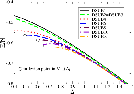
Figure 2: (Color online) CCM results for the ground-state energy per spin, $E/N$, as a function of the anisotropy parameter $\Delta$, of the spin-$1/2$ $XXZ$ model on the square lattice, using various DSUBm approximations based on the z-aligned Néel model state. The DSUB$m$ results with $m=\{6,8,10\}$ are extrapolated using the leading (linear) fit of equation (22) and shown as the curve DSUB$\infty$. $\Delta_{i}\equiv$ magnetization point of inflexion, described in the text.

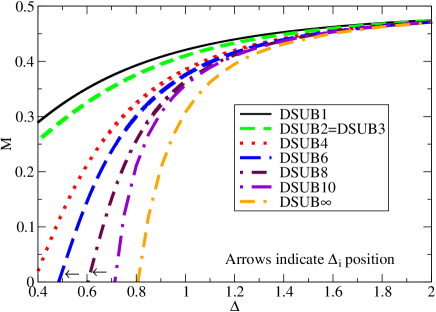
Figure 3: (Color online) CCM results for the sublattice magnetization, $M$, as a function of the anisotropy parmeter $\Delta$, of the spin-$1/2$ $XXZ$ model on the square lattice, using various DSUBm approximations based on the z-aligned Néel model state. The DSUB$m$ results with $m=\{6,8,10\}$ are extrapolated using the leading (linear) fit of equation (23) and shown as the curve DSUB$\infty$. $\Delta_{i}\equiv$ point of inflexion in the curve, shown by arrows in the figure.

We also show in table 2 for the isotropic Heisenberg Hamiltonian ($\Delta=1$) the results for the gs energy and sublattice magnetization using the leading (linear) extrapolation schemes of equations (22) and (23) respectively of the DSUB$m$ data, employing various subsets of results. Comparison is also made with corresponding LSUB$m$ extrapolation schemes for the same model [34, 35]. The results are generally observed to be in excellent agreement with each other, even though the DSUB$\infty$ extrapolations have employed the simple leading (linear) fits of equations (22) and (23), whereas the corresponding LSUB$\infty$ results shown [34, 35] have been obtained from the potentially more accurate quadratic fits $E/N=a_{0}+a_{1}(1/m^{2})+a_{2}(1/m^{2})^{2}$, $M=b_{0}+b_{1}(1/m^{2})+b_{2}(1/m)^{2}$, to the LSUB$m$ data, in which the next-order (quadratic) corrections have also been included in the relevant expansion parameters, $1/m^{2}$ and $1/m$, respectively. Excellent agreement of all the CCM extrapolations is also obtained with the results from the best of the alternative methods for this model, including third-order spin-wave theory (SWT) [36], linked-cluster series expansion techniques [38], and the extrapolations to infinite lattice size ($N\rightarrow\infty$) from the exact diagonalization (ED) of small lattices [37], and quantum Monte Carlo (QMC) calculations for larger lattices [40].

We note that it has been observed and well documented in the past (and see, e.g., Ref. [34]) that the CCM LSUB$m$ results for this model (and many others) for both the gs energy $E$ and the sublattice magnetization $M$ show a distinct period-2 ‘‘staggering’’ effect with index $m$, according to whether $m$ is even or odd. As a consequency the LSUB$m$ data for both $E$ and $M$ converge differently for the even-$m$ and the odd-$m$ sequences, similar to what is observed very frequently in perturbation theory in corresponding even and odd orders [40]. As a rule, therefore, the LSUB$m$ data are generally extrapolated separately for even $m$ and for odd values of $m$, since the staggering makes extrapolations using both odd and even values together extremely difficult. We show in figure 4

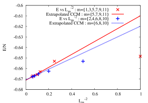
(a) Ground-state energy per spin

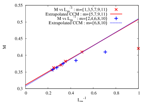
(b) Ground-state sublattice magnetization

Figure 4: (Color online) Illustration of the staggered nature of the DSUB$m$ scheme for the gs energy per spin, $E/N$, and sublattice magnetization, $M$, for the spin-$1/2$ antiferromagnetic $XXZ$ model on the square lattice. The DSUB$m$ data are plotted against $1/L_{m}^{2}$ for $E/N$ and against $1/L_{m}$ for $M$. The results clearly justify the heuristic extrapolation schemes of equations (22) and (23).

our DSUB$m$ results for the gs energy per spin and the sublattice magnetization plotted against $1/L^{2}_{m}$ and $1/L_{m}$, respectively. The higher $m$ values clearly cluster well in both cases on straight lines, thereby justifying a posteriori our heuristic extrapolation fits of equations (22) and (23). Just as in the LSUB$m$ case a slight ‘‘even-odd staggering’’ effect is observed in the DSUB$m$ data (perhaps more so for the energy than for the sublattice magnetization), although it is less pronounced than for the corresponding LSUB$m$ data [34].

6.2 Termination or critical points

Before discussing our DSUB$m$ results further for this model we note that the comparable LSUB$m$ solutions actually terminate at a critical value $\Delta_{c}=\Delta_{c}(m)$, which itself depends on the truncation index $m$ [30]. Such LSUB$m$ termination points are very common for many spin-lattice systems and are very well documented and understood (and see, e.g., Ref. [30]). In all such cases a termination point always arises due to the solution of the CCM equations becoming complex at this point, beyond which there exist two branches of entirely unphysical complex conjugate solutions [30]. In the region where the solution reflecting the true physical solution is real there actually also exists another (unstable) real solution. However, only the (shown) upper branch of these two solutions reflects the true (stable) physical GS, whereas the lower branch does not. The physical branch is usually easily identified in practice as the one which becomes exact in some known (e.g., perturbative) limit. This physical branch then meets the corresponding unphysical branch at some termination point beyond which no real solutions exist. The LSUB$m$ termination points are themselves also reflections of the quantum phase transitions in the real system, and may be used to estimate the position of the phase boundary [30].

It is interesting and intriguing to note that when the DSUB$m$ approximations are applied to the $XXZ$ model, they do not terminate as do the corresponding LSUB$m$ approximations. We have no real explanation for this rather striking difference in behaviour for two apparently similar schemes applied to the same model. However, it is still possible to use our DSUB$m$ data to extract an estimate for the physical phase transition point at which the $z$-aligned Néel phase terminates. As has been justified and utilized elsewhere [18], a point of inflexion at $\Delta=\Delta_{i}$ in the sublattice magnetization $M$ as a function of $\Delta$ clearly indicates the onset of an instability in the system. Such inflexion points $\Delta_{i}=\Delta_{i}(m)$ occur for all DSUB$m$ approximations, as indicated in table 2 and figure 3. The DSUB$m$ approximations are thus expected to be unphysical for $\Delta<\Delta_{i}(m)$, and we hence show the corresponding results for the gs energy per spin in figure 2 only for values $\Delta_{i}>\Delta_{i}(m)$. Heuristically, we find that the magnetization inflexion points $\Delta_{i}(m)$ scale linearly with $1/L_{m}$ to leading order, and the extrapolated results shown in table 2 have been performed with the leading (linear) fit, $\Delta_{i}=c_{o}+c_{1}(1/L_{m})$, commensurate with the corresponding linear fits in $(1/L^{2}_{m})$ and $(1/L_{m})$ for the gs energy per spin and sublattice magnetization of equations (22) and (23), respectively. All of the various extrapolations shown in table 2 for $\Delta_{i}$ in the limit $m\rightarrow\infty$ are in good agreement with one another, thereby again demonstrating the robust quality of the heuristic extrapolation scheme. Furthermore, they are also in excellent agreement with the expected phase transition point at $\Delta_{c}\equiv 1$ between two quasiclassical Néel-ordered phases aligned along the spin $z$-axis (for $\Delta>1$) and in some arbitrary direction in the spin $x$-$y$-plane (for $|\Delta|<1$).

Although we do not do so here, the $x$-$y$ planar Néel phase could itself also easily be investigated by another CCM DSUB$m$ series of calculations based on a model state $|\Phi\rangle$ with perfect Néel ordering in, say, the $x$-direction.

Summarizing our results so far, we observe that the DSUB$m$ scheme has at, least partially, fulfilled the expectations placed upon it for the present model. Accordingly, we now apply it to the second test model of the spin-1/2 $XY$ model on the 2D square lattice.

7 The spin-1/2 $XY$ model on the square lattice

The Hamiltonian of the $XY$ model [18] in global spin coordinates, is written as

$$H_{XY}=\sum_{\langle i,j\rangle}[(1+\Delta)s^{x}_{i}s^{x}_{j}+(1-\Delta)s^{y}_{i}s^{y}_{j}]\,;\hskip 14.45377pt-1\leq\Delta\leq 1\,,$$ (27)

where the sum on $\langle i,j\rangle$ again runs over all nearest-neighbour pairs of lattice sites and counts each pair only once. We again consider the case of spin-1/2 particles on each site of an infinite square lattice.

For the classical model described by equation (27), it is clear that the GS is a Néel state in the $x$-direction for $0<\Delta\leq 1$ and a Néel state in the $y$-direction for $-1\leq\Delta<0$. Hence, since we only consider the case $0\leq\Delta\leq 1$, we choose as our CCM model state $|\Phi\rangle$ for the quantum $XY$ model a Néel state aligned along the $x$-direction, written schematically as,

$$|\Phi\rangle=|\cdots\leftarrow\,\rightarrow\,\leftarrow\,\rightarrow\cdots\rangle\;,\hskip 14.45377pt\mbox{in the global spin axes}.$$

Clearly the case $-1\leq\Delta<0$ is readily obtained from the case $0<\Delta\leq 1$ by interchange of the $x$- and $y$-axes.

Once again we now perform our usual rotation of the spin axes on each lattice site so that $|\Phi\rangle$ takes the form given by equation (19) in the rotated local spin coordinate frame. Thus, for the spins on the sublattice where they point in the negative $x$-direction in the global spin axes (i.e., the left-pointing spins) we perform a rotation of the spin axes by $+90^{\circ}$ about the spin $y$-axis. Similarly, for the spins on the other sublattice where they point in the positive $x$-direction in the global spin axes (i.e., the right-pointing spins) we perform a rotation of the spin axes by $-90^{\circ}$ about the spin $y$-axis. Under these rotations the spin operators are transformed as

$$s^{x}\rightarrow s^{z}\;,\qquad s^{y}\rightarrow s^{y}\;,\qquad s^{z}\rightarrow-s^{x}\;,\qquad\mbox{left-pointing spins};$$ (28a)

$$s^{x}\rightarrow-s^{z}\;,\qquad s^{y}\rightarrow s^{y}\;,\qquad s^{z}\rightarrow s^{x}\;,\qquad\mbox{right-pointing spins}.$$ (28b)

The Hamiltonian of equation (27) may thus be rewritten in the local spin coordinate axes defined above as

$$H_{XY}=\sum_{\langle i,j\rangle}\left[-(1+\Delta)s^{z}_{i}s^{z}_{j}-\frac{1}{4}(1-\Delta)(s^{+}_{i}s^{+}_{j}+s^{-}_{i}s^{-}_{j})+\frac{1}{4}(1-\Delta)(s^{+}_{i}s^{-}_{j}+s^{-}_{i}s^{+})\right]\;.$$ (29)

As before, we now have to evaluate the fundamental configurations that are retained in the CCM correlation operators $S$ and $\tilde{S}$ at each DSUB$m$ level of approximation. Although the point and space group symmeries of the square lattice (common to both the $XXZ$ and $XY$ models considered here) and the two Hamiltonians of equations (26) and (29) are identical, the numbers $N_{f}$ of fundamental configurations for a given DSUB$m$ level are now larger (except for the case $m=1$) for the $XY$ model than for the $XXZ$ model, since the uniform magnetization is no longer a good quantum number for the $XY$ model, $[H_{XY},S^{z}_{T}]\neq 0$. Nevertheless, we note from the form of equation (29), in which the spin-raising and spin-lowering operators appear only in combinations that either raise or lower the number of spin flips by two (viz., the $s^{+}_{i}s^{+}_{j}$ and $s^{-}_{i}s^{-}_{j}$ combinations, respectively) or leave them unchanged (viz., the $s^{+}_{i}s^{-}_{j}$ and $s^{-}_{i}s^{+}_{j}$ combinations), it is only necessary for the $s^{z}_{T}=0$ GS to consider fundamental configurations that contain an even number of spins. Thus, the main difference for the $XY$ model over the $XXZ$ model is that we must now also consider fundamental configurations in which we drop the restriction for the former case of having an equal number of spins on the two equivalent sublattices of the bipartite square lattice that was appropriate for the latter case. We show in figure 5 the fundamental configurations that are allowed for the spin-1/2 $XY$ model on the square lattice for the DSUB$m$ approximation with $1\leq m\leq 3$, and we invite the reader to compare with the corresponding fundamental configurations for the spin-1/2 $XXZ$ model on the same square lattice shown in figure 1.

Figure 5: The fundamental configurations for the DSUB$m$ scheme with $m=\{1,2,3\}$ for the spin-1/2 $XY$ model on a square lattice in two dimensions. The filled circles mark the relative positions of the sites of the square lattice on which the spins are flipped with respect to the model state. The unfilled circles represent unflipped sites.

The corresponding numbers $N_{f}$ of fundamental configurations for the $XY$ model are also shown in table 3 for the higher DSUB$m$ approximations with $m\leq 9$ for which we present results below.

7.1 Ground-state energy and sublattice magnetization

We present results for the spin-1/2 $XY$ model on the square lattice in the CCM DSUB$m$ approximations for all values $m\leq 9$ that can be easily computed with very modest computing power. Comparable computing power enables the corresponding LSUB$m$ scheme to be implemented for all $m\leq 8$. Numerical results for the gs energy per spin and sublattice magnetization are shown in table 3 at the isotropic point at $\Delta=0$ at various levels of approximation, and corresponding results for the same gs quantities are shown graphically in figures 6 and 7 as functions of the anisotropy parameter $\Delta$.

Table 3: The ground-state energy per spin ($E/N$) and sublattice magnetization ($M$) for the spin-$1/2$ $XY$ model on the square lattice, obtained using the CCM DSUB$m$ approximation scheme with $1\leq m\leq 9$ at $\Delta=0$. $N_{f}$ is the number of fundamental configurations at a given level of DSUB$m$ or LSUB$m$ approximation. $\Delta_{c}\equiv$ DSUB$m$ termination point. The DSUB$m$ results for odd values of $m$, even values of $m$ and the whole series of $m$ are extrapolated separately. These results are compared to calculations of series expansion (SE), quantum Monte Carlo (QMC) and LSUB$\infty$ extrapolations of the CCM LSUB$m$ approximations.

Method	$L_{m}$	$N_{f}$	$E/N$	$M$	$\Delta_{c}$	Max. No.
			$\Delta=0$			of spins
DSUB1=LSUB2	1	1	-0.54031	0.475		2
DSUB2	$\sqrt{2}$	3	-0.54425	0.467		4
DSUB3	2	6	-0.54544	0.464		4
DSUB4	$\sqrt{5}$	21	-0.54724	0.458	-0.253	6
DSUB5	$\sqrt{8}$	44	-0.54747	0.456	-0.205	8
DSUB6	3	78	-0.54774	0.455	-0.181	8
DSUB7	$\sqrt{10}$	388	-0.54811	0.453	-0.135	12
DSUB8	$\sqrt{13}$	1948	-0.54829	0.451	-0.107	14
DSUB9	4	3315	-0.54833	0.451	-0.099	14
LSUB6		131	-0.54833	0.451	-0.073	6
LSUB8		2793	-0.54862	0.447	-0.04	8
	Extrapolations
	Based on		$E/N$	$M$		$\Delta_{c}$
DSUB$\infty$	$m=\{4,6,8\}$		-0.54879	0.442		-0.036
DSUB$\infty$	$m=\{5,7,9\}$		-0.54923	0.437		0.011
DSUB$\infty$	$4\leq m\leq 9$		-0.54884	0.441		-0.029
LSUB$\infty$ [18]	$m=\{4,6,8\}$		-0.54892	0.435		0.00
SE [41]			-0.54883	0.43548		0.0
QMC [42]			-0.548824(2)	0.437(2)

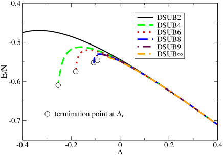
Figure 6: (Color online) CCM results for the gs energy of the spin-$1/2$ $XY$ model on the square lattice obtained using the DSUBm approximation based on the Néel state aligned along any axis in the $x$-$y$ plane. The DSUB$m$ results with $m=\{5,7,9\}$ are extrapolated using equation (22) to give the curve labelled DSUB$\infty$.

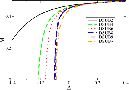
Figure 7: (Color online) CCM results for the gs sublattice magnetization of the spin-$1/2$ $XY$ model on the square lattice obtained using various DSUBm approximations based on the Néel state aligned along any axis in the $x$-$y$ plane. The DSUB$m$ results with $m=\{5,7,9\}$ are extrapolated using equation (23) to give the curve labelled DSUB$\infty$.

We also show in table 3 for the isotropic $XY$ Hamiltonian ($\Delta=0$) the results for the gs energy and sublattice magnetization using the leading (linear) extrapolation schemes of equations (22) and (23) respectively of the DSUB$m$ data, employing various subsets of our results, as for the $XXZ$ model considered previously. We also compare in table 3 the present results with the corresponding CCM LSUB$m$ results [18] for the same model. All of the CCM results are clearly in excellent agreement both with one another and with the results of best of the alternative methods available for this model, including the linked-cluster series expansion (SE) techniques [41] and a quantum Monte Carlo (QMC) method [42].

We again show in figure 8 our DSUB$m$ results for the present $XY$ model for the gs energy per spin and the sublattice magnetization, plotted respectively against $1/L^{2}_{m}$ and $1/L_{m}$.

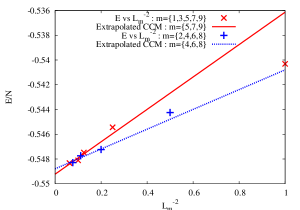
(a) Ground-state energy per spin

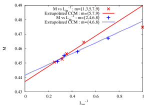
(b) Ground-state sublattice magnetization

Figure 8: (Color online) Illustration of the staggered nature of the DSUB$m$ scheme for the gs energy per spin, $E/N$, and sublattice magnetization, $M$, for the spin-$1/2$ $XY$ model on the square lattice. The DSUB$m$ data are plotted against $1/L_{m}^{2}$ for $E/N$ and against $1/L_{m}$ for $M$. The results clearly justify the heuristic extrapolation schemes of equations (22) and (23).

As previously for the $XXZ$ model, the higher $m$ values cluster well on straight lines in both cases, thereby justifying once more our heursitic choice of extrapolation fits indicated in equations (22) and (23). Figures 8(a) and 8(b) again show an ‘‘even-odd’’ staggering effect in the termination index $m$ for the DSUB$m$ data, which is perhaps slightly more pronounced than that for the $XXZ$ model shown in figures 4(a) and 4(b). For this reason we have again shown separate extrapolations of our DSUB$m$ results in table 3 for the even-$m$ data and the odd-$m$ data, as well as results using all (higher) values of $m$.

7.2 Termination or critical points

It is interesting to note that for the present $XY$ model the CCM DSUB$m$ solutions (with our choice of model state as a Néel state in the $x$-direction) now do physically terminate for all values of the truncation index $m\geq 4$ at a critical value $\Delta_{c}=\Delta_{c}(m)$, exactly as commonly occurs (as for the present model) for the LSUB$m$ calculations, as we explained above in section 6.2. Why such DSUB$m$ terminations occur for the $XY$ model but not for the previous $XXZ$ model is not obvious to us. The corresponding termination points, $\Delta_{c}=\Delta_{c}(m)$, at various DSUB$m$ and LSUB$m$ levels of approximation are shown in table 3. It has been shown previously [29] that $\Delta_{c}(m)$ scales well with $1/m^{2}$ for the LSUB$m$ data, and the LSUB$\infty$ result [18] shown in table 3 was obtained by a leading (linear) fit, $\Delta_{c}(m)=d_{0}+d_{1}(1/m^{2})$. We find heuristically that the best large-$m$ asymptotic behaviour of the DSUB$m$ data for $\Delta_{c}(m)$ is against $1/L^{2}_{m}$ as the scaling parameter. Accordingly, the DSUB$\infty$ values for $\Delta_{c}$ in table 3 are obtained with the leading (linear) fit, $\Delta_{c}(m)=d_{0}+d_{1}(1/L_{m}^{2})$. We see that both the LSUB$\infty$ and DSUB$\infty$ results for $\Delta_{c}\equiv\Delta_{c}(\infty)$ agree very well with the value $\Delta_{c}=0$ that is known to be the correct value for the phase transition in the one-dimensional spin-1/2 $XY$ chain from the known exact solution [43], and which is believed also to be the phase transition point for higher dimensions, including the present 2D square lattice, on symmetry grounds.

8 Conclusions

From the two nontrivial benchmark spin-lattice problems that we have investigated here, it is clear that the new DSUB$m$ approximation scheme works well for calculating their gs properties and phase boundaries. We have utilized here only the simplest leading-order extrapolation schemes in the pertinent scaling variables, and have shown that these may be chosen, for example, as $1/L^{2}_{m}$ for the gs energy and $1/L_{m}$ for the order parameter. Clearly, in general, the results can be further improved by keeping higher-order terms in these asymptotic expansions (i.e., by retaining higher powers in the polynomial scaling expansions) although more data points may then be needed, especially in cases where the ‘‘even-odd’’ staggering effect is pronounced, as for $XY$ model presented here. For further use of the scheme for more complex lattice models (e.g., those exhibiting geometric or dynamic frustration) it will be necessary to re-visit the validity of these expansions, but a great deal of previous experience in such cases for the LSUB$m$ scheme will provide good guidance.

On the basis of the test results presented here, the DSUB$m$ scheme clearly fulfills the first of our two main criteria for introducing it, viz., that the number of fundamental configurations, $N_{f}$, increases less rapidly with truncation index $m$ than for the corresponding LSUB$m$ series of approximations. At the same time our second criterion of capturing the physically most important configurations at relatively low levels of approximation also seems to be fulfilled, according to our experience with the convergence of the DSUB$m$ sequences for observable quantities. At the very least we now have two schemes (LSUB$m$ and DSUB$m$) available to us for future investigations, each of which has its own merits, and which thus allows us more freedom in applications of the CCM to other spin-lattice models in future.

The one slight drawback in the scheme which mitigates against our goal of obtaining more DSUB$m$ data points, for the same computing power than for the LSUB$m$ scheme applied to the same system, and that hence can be used together to attain more accuracy in the extrapolations, is the slight ‘‘even-odd’’ staggering in the data that is observed in the DSUB$m$ results, albeit that it is somewhat reduced from the similar stagerring in the corresponding LSUB$m$ results. We have some ideas on how the DSUB$m$ scheme might itself be modified to reduce this staggering and we hope to report results of these further investigations in a future paper.

References

- 1. Coester F., Nucl. Phys., 1958, 7, 421.
- 2. Čížek J., J. Chem. Phys., 1966, 45, 4256.
- 3. Paldus J., Čížek J., Shavitt I., Phys. Rev. A, 1972, 5, 50.
- 4. Kümmel H., Lührmann K.H., Zabolitzky J.G., Phys. Rep., 1978, 36C, 1.
- 5. Arponen J.S., Ann. Phys. (N.Y.), 1983, 151, 311.
- 6. Arponen J.S., Bishop R.F., Pajanne E., Phys. Rev. A, 1987, 36, 2539.
- 7. Bartlett R.J., J. Phys. Chem., 1989, 93, 1697.
- 8. Bishop R.F., Theor. Chim. Acta, 1991, 80, 95.
- 9. Bishop R.F., in Microscopic Quantum Many-Body Theories and Their Applications, eds. Navarro J., Polls A., Lecture Notes in Physics, 1998, 510, Springer-Verlag, Berlin, p.1.
- 10. Bishop R.F., Lührmann K.H., Phys. Rev. B, 1978, 17, 3757.
- 11. Bishop R.F., Lührmann K.H., Phys. Rev. B, 1982, 26, 5523.
- 12. Day B.D., Phys. Rev. Lett., 1981, 47, 226.
- 13. Day B.D., Zabolitzky J.G., Nucl. Phys., 1981, A336, 221.
- 14. Bartlett R.J., Ann. Rev. Phys. Chem., 1981 32, 359.
- 15. Roger M., Hetherington J.H., Phys. Rev. B, 1990, 41, 200.
- 16. Bishop R.F., Parkinson J.B., Xian Y., Phys. Rev. B, 1991, 44, 9425.
- 17. Bursill R., Gehring G.A., Farnell D.J.J., Parkinson J.B., Xiang T., Zeng C., J. Phys.: Condens. Matter, 1995, 7, 8605.
- 18. Farnell D.J.J., Krüger S.E., Parkinson J.B., J. Phys.: Condens. Matter, 1997, 9, 7601.
- 19. Bishop R.F., Farnell D.J.J., Parkinson J.B., Phys. Rev. B, 1998, 58, 6394.
- 20. Bishop R.F., Farnell D.J.J., Krüger S.E., Parkinson J.B., Richter J., Zeng C., J. Phys.: Condens. Matter, 2000, 12, 6887.
- 21. Farnell D.J.J., Gernoth K.A., Bishop R.F., Phys. Rev. B, 2001, 64, 172409.
- 22. Farnell D.J.J., Bishop R.F., Gernoth K.A., J. Stat. Phys., 2002, 108, 401.
- 23. Bishop R.F., Li P.H.Y., Darradi R., Richter J., J. Phys.: Condens. Matter, 2008, 20, 255251.
- 24. Bishop R.F., Li P.H.Y., Darradi R., Richter J., Europhys. Lett., 2008 83, 47004.
- 25. Bishop R.F., Li P.H.Y., Darradi R., Schulenburg J., Richter J., Phys. Rev. B, 2008, 78, 054412.
- 26. Bishop R.F., Li P.H.Y., Darradi R., Richter J., Campbell C.E., J. Phys.: Condens. Matter, 2008, 20, 415213.
- 27. Bishop R.F., Li P.H.Y., Farnell D.J.J., Campbell C.E., Phys. Rev. B, 2009, 79 (in press).
- 28. Bishop R.F., Parkinson J.B., Xian Yang, Phys. Rev. B, 1991, 43, 13782.
- 29. Bishop R.F., Hale R.G., Xian Y., Phys. Rev. Lett., 1994, 73, 3157.
- 30. Farnell D.J.J., Bishop R.F., in Quantum Magnetism, eds. Schollwöck U., Richter J., Farnell D.J.J., Bishop R.F., Lecture Notes in Physics, 2004, 645, Springer-Verlag, Berlin, p.307.
- 31. Zeng C., Farnell D.J.J., Bishop R.F., J. Stat. Phys., 1998, 90, 327.
- 32. Krüger S.E., Richter J., Schulenburg J., Farnell D.J.J., Bishop R.F., Phys. Rev. B, 2000, 61, 14607.
- 33. Schmalfuß D., Darradi R., Richter J., Schulenburg J., Ihle D., Phys. Rev. Lett., 2006, 97, 157201.
- 34. Farnell D.J.J., Bishop R.F., Int. J. Mod. Phys. B, 2008, 22, 3369.
- 35. Richter J., Darradi R., Zinke R., Bishop R.F., Int. J. Mod. Phys. B, 2007, 21, 2273.
- 36. Hamer C.J., Weihong Z., Arndt P., Phys. Rev. B, 1992, 46, 6276.
- 37. Weihong Z., Oitmaa J., Hamer C.J., Phys. Rev. B, 1991, 43, 8321.
- 38. Richter J., Schulenburg J., Honecker A., in Quantum Magnetism, eds. Schollwöck U., Richter J., Farnell D.J.J., Bishop R.F., Lecture Notes in Physics, 2004, 645, Springer-Verlag, Berlin, p.85.
- 39. Sandvik A.W., Phys. Rev. B, 1997, 56, 11678.
- 40. Morse P.M., Feshbach H., Methods of Theoretical Physics, Part II, 1953, McGraw-Hill, New York.
- 41. Hamer C.J., Oitmaa J., Weihong Z., Phys. Rev. B, 1991, 43, 10789.
- 42. Sandvik A.W., Hamer C.J., Phys. Rev. B, 1999, 60, 6588.
- 43. Lieb E., Schultz T., Mattis D., Ann. Phys. (N.Y.), 1961, 16, 407.