Information of Interest

Abstract

A pricing formula for discount bonds, based on the consideration of the market perception of future liquidity risk, is established. An information-based model for liquidity is then introduced, which is used to obtain an expression for the bond price. Analysis of the bond price dynamics shows that the bond volatility is determined by prices of certain weighted perpetual annuities. Pricing formulae for interest rate derivatives are derived.

Working paper. This version: .

Email: dorje@imperial.ac.uk, robyn.freidman@rbs.com

1. Introduction. We would like to present here an idea concerning how to generate interest rate dynamics from elementary economic considerations. There are of course numerous economic factors that affect the movement of interest rates, and causal relations that hold between these factors are often difficult to disentangle. Hence, rather than attempting to address a range of factors simultaneously, we will focus on one key factor that appears important in determining the interest rate term structure; namely, the liquidity risk, in the narrow sense of cash demand. Our objective is to build an information-based model that reflects the market perception of future liquidity risk, and use it for the pricing and general risk management of interest rate derivatives.

In the framework of arbitrage-free pricing theory the value of an asset is determined by the risk-adjusted expectation of the suitably discounted cash flow. Thus in principle one can derive the price process of an asset by the specification of the random cash flow, along with the market filtration and the discounting factor. Such an idea has been applied successfully to obtain the price process of, for example, credit-risky bonds (Brody et al. 2007) or reinsurance-related products (Brody et al. 2008). When it comes to the modelling of interest rate term structure, however, the matter is made somewhat more complicated, because the cash flow of a discount bond is not random, and thus one has to specify the discount factor to deduce the bond price. One is then led to the specification of the short rate or forward rate processes, but such an approach is undesirable if the objective is to generate from the outset the dynamics of the term structure. This forces us to take an alternative route for deriving bond prices and the associated rates.

The new pricing framework outlined here, based on the consideration of liquidity risk, has several advantages worth noting: (i) economic interpretations of the discount function, the associated rates, and their volatilities become intuitive; (ii) initial term structure can be specified exogenously in a straightforward manner; (iii) arbitrage-free dynamics of interest rates emerge endogenously in such a manner that they are consistent with the market perception of future cash demand; (iv) semi-analytic formulae for caplet and swaption, expressed in terms of elementary Gaussian integrations, can be obtained; and (v) risk premium can in principle be estimated from prices of interest rate derivatives. To illustrate the role played by liquidity risk in determining interest rate systems, let us begin by examining deterministic term structures.

2. Deterministic term structures. Consider first the initial discount function $P_{0T}$. It should be evident that positivity of nominal rates implies that the discount function $P_{0T}$ is decreasing in the maturity variable $T$. Furthermore, a common sense argument shows that a bond with infinite maturity has no value. Thus $P_{0T}$ can be thought of as defining a right-side cumulative distribution function on the positive real line ${\mathds{R}}_{+}$. In particular, $\rho_{0}(T)=-\partial_{T}P_{0T}$ defines a density function over ${\mathds{R}}_{+}$. Put the matter differently, the positive interest term structure implies the existence of a random variable $X$ on a probability space with measure ${\mathbb{Q}}$ such that we have $P_{0T}={\mathbb{Q}}(X\geq T)$. Based on this observation a general arbitrage-free dynamical equation satisfied by the term structure density process $\rho_{t}(T)=-\partial_{T}P_{tT}$ was obtained by Brody & Hughston (2001). In the present investigation, however, we would like to pay more attention to the interpretation of the cumulative distribution $P_{0T}$, the meaning of the random variable $X$, and the role of the probability measure ${\mathbb{Q}}$, in such a way that new interest rate models can be created.

We remark that it is reasonable to regard the random variable $X$ as representing the occurrence time of future liquidity issues, at least to first approximation. From the viewpoint of the buyer of a bond, if with high probability cash is needed before the maturity $T$, then purchase will be made only if the bond price is sufficiently low. Likewise, the seller of a bond would be willing to pay a high premium if there is a likely need for cash before time $T$. Thus $P_{0T}$ represents a survival function, where ‘survival’ means lack of liquidity crisis. It is worth noting that the interplay between liquidity and interest rate has long been discussed in the economics literature. To this end we refer to the presidential address delivered at the eightieth annual meeting of the American Economic Association (Friedman 1968) for further insights.

What we would like to establish here is the fact that the price of a discount bond with maturity $T$ is determined by the risk-adjusted probability that the liquidity crisis arises beyond time $T$: $P_{0T}={\mathbb{Q}}(X\geq T)$. That ${\mathbb{Q}}$ represents the risk-neutral measure will be shown later, but let us for the moment assume that this is the case. Then the risk-neutral hazard rate associated with liquidity crisis is just the initial forward rate $f_{0T}$. Therefore, for a small $\mbox{$\rm d$}T$ we have

$$f_{0T}\,\mbox{$\rm d$}T={\mathbb{Q}}\left(X\in[T,T+\mbox{$\rm d$}T]\,|\,X\geq T\right).$$ (1)

In other words, $f_{0T}\,\mbox{$\rm d$}T$ is the a priori risk-neutral probability of a liquidity crisis occurring in an infinitesimal interval $[T,T+\mbox{$\rm d$}T]$, conditional upon survival until time $T$.

More generally, in the case of a deterministic interest rate term structure, the price $P_{tT}$ at time $t$ of a bond that matures at $T$ is given by the risk-neutral probability of survival until $T$ conditional on survival until $t$:

$$P_{tT}={\mathbb{Q}}\left(X\geq T\,|\,X\geq t\right).$$ (2)

This can be verified by use of the Bayes formula, which shows that the right side of (2) is given by $P_{0T}/P_{0t}$. But this is just the bond price $P_{tT}$ in the case of a deterministic term structure. Thus in a deterministic interest rate system we can calibrate the initial term structure density $\rho_{0}(T)$ using the initial yield curve, from which the subsequent evolution is determined in accordance with (2).

3. Market information about future liquidity. Our aim now is to extend the deterministic model (2) into a dynamical one without losing the key economic interpretation. That is to say, we would like to retain the fact that the bond price represents the conditional risk-neutral probability that the liquidity issue arises beyond time $T$. The problem therefore is to identify the relevant conditioning. In the case of a deterministic term structure (2) the conditioning is given merely by the event $X\geq t$. In a dynamical setup, however, market participants accumulate noisy information concerning future liquidity risk. It is this noisy observation of the timing $X$ of the future cash demand that generates random movements in the bond price. Thus if we let $\{{\mathcal{F}}_{t}\}$ denote the information generated by this observation, then the price of a discount bond is given by the conditional probability

$$P_{tT}={\mathbb{Q}}\left(X\geq T\,|\,(X\geq t)\cap{\mathcal{F}}_{t}\right).$$ (3)

Evidently, the random variable representing the timing of cash demand itself may change in time. In the present investigation, however, we shall confine our analysis to models based on fixed $X$.

If we apply the Bayes formula, then (3) can be expressed in a more intuitive form

$$P_{tT}=\frac{{\mathbb{Q}}\left(X\geq T|{\mathcal{F}}_{t}\right)}{{\mathbb{Q}}\left(X\geq t|{\mathcal{F}}_{t}\right)}.$$ (4)

This is the pricing formula for a discount bond that we propose here. In obtaining (4) we have made use of the fact that $(X\geq T)\cap(X\geq t)=(X\geq T)$.

4. An elementary model for bond price. To proceed we introduce a specific model for $\{{\mathcal{F}}_{t}\}$. Since in the present formulation what concerns market participants is the value of $X$, the ‘signal’ component of the observation must be generated in some form by $X$ itself. In addition, there is an independent noise that obscures the value of $X$. Motivated by the approach introduced in Macrina (2006) and in Brody et al. (2007) for the information-based asset pricing framework, let us consider a simple model whereby the information concerning the value of $X$ is revealed to the market linearly in time at a constant rate $\sigma$, and the noise is generated by an independent Brownian motion $\{B_{t}\}$, defined on a probability space with measure ${\mathbb{Q}}$. Thus the information generating process is given by

$$\xi_{t}=\sigma t\phi(X)+B_{t},$$ (5)

where $\phi(x)$ is a smooth invertible function. In other words, we assume that the filtration ${\mathcal{F}}_{t}$ is given by the sigma algebra generated by $\{\xi_{s}\}_{0\leq s\leq t}$. Note that a more coherent formulation is obtained if we replace the Brownian noise $B_{t}$ by a ‘killed’ Brownian noise ${\mathds{1}}\{X\geq t\}B_{t}$. However, since we are interested in events on $\{X\geq t\}$, and since this alternation does not affect the bond pricing formula, we shall be using (5) for simplicity of exposition. As regards the choice of the function $\phi(x)$ we shall have more to say shortly, but let us for the moment proceed with generality.

We note that since the magnitude of the signal-to-noise ratio is given by $\sigma\sqrt{t}$, the value of $X$ will be revealed asymptotically, that is, $X$ is ${\mathcal{F}}_{\infty}$-measurable. Along with the fact that $\{\xi_{t}\}$ of (5) is Markovian, we find that the bond pricing formula simplifies in this model to

$$P_{tT}=\frac{{\mathbb{Q}}\left(X\geq T|\xi_{t}\right)}{{\mathbb{Q}}\left(X\geq t|\xi_{t}\right)}.$$ (6)

For the calculation of the bond price (6) we consider the following joint probability ${\mathbb{Q}}\left((X\geq T)\cap(\xi_{t}\in\mbox{$\rm d$}\xi)\right)$. Then, on account of the definition (5), we have

$${\mathbb{Q}}\left((X\geq T)\cap(\xi_{t}\in\mbox{$\rm d$}\xi)\right)=\int_{T}^{\infty}{\mathbb{Q}}\left(B_{t}\in[\mbox{$\rm d$}\xi-\sigma t\phi(x)]\right)\rho_{0}(x)\mbox{$\rm d$}x,$$ (7)

where $\rho_{0}(x)=-\partial_{x}P_{0x}$ is the initial term structure density. By substituting the density function for the Brownian motion we obtain the following expression:

$$P_{tT}=\frac{\int_{T}^{\infty}\rho_{0}(x)\,\mbox{$\rm e$}^{\sigma\phi(x)\xi_{t}-\frac{1}{2}\sigma^{2}\phi^{2}(x)t}\mbox{$\rm d$}x}{\int_{t}^{\infty}\rho_{0}(x)\,\mbox{$\rm e$}^{\sigma\phi(x)\xi_{t}-\frac{1}{2}\sigma^{2}\phi^{2}(x)t}\mbox{$\rm d$}x}.$$ (8)

It is interesting to observe that the form of the bond price thus obtained is closely related to the general positive interest representation obtained by Flesaker & Hughston (1996).

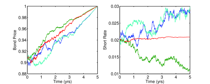
Figure 1: Sample paths of the discount function (8) and the associated short rate (9). The information-adjusting function is set as $\phi(x)=\mbox{$\rm e$}^{-0.025x}$, and the initial term structure is assumed flat so that $P_{0T}=\mbox{$\rm e$}^{-0.02T}$. The information flow rate is set as $\sigma=0.3$, and the bond maturity is 5 years.

As in the deterministic case, the model can be calibrated exactly against the initial yield curve according to the prescription $\rho_{0}(x)=-\partial_{x}P_{0x}$. The subsequent evolution is then determined by the Markovian market information process. In this respect the model has a feature resembling the Markov-functional models (Hunt & Kennedy 2000). The remaining degree of freedom, namely, the parameter $\sigma$, can be calibrated by use of derivative prices. This will be discussed later.

From the bond price (8) we can infer the implied short rate $r_{t}=-\partial_{T}P_{tT}|_{T=t}$. This is given by

$$r_{t}=\frac{\rho_{0}(t)\,\mbox{$\rm e$}^{\sigma\phi(t)\xi_{t}-\frac{1}{2}\sigma^{2}\phi^{2}(t)t}}{\int_{t}^{\infty}\rho_{0}(x)\,\mbox{$\rm e$}^{\sigma\phi(x)\xi_{t}-\frac{1}{2}\sigma^{2}\phi^{2}(x)t}\mbox{$\rm d$}x}.$$ (9)

We draw attention to the observation made in Brody & Hughston (2001) that the short rate is the negative expectation of the differential operator $\partial_{X}=\partial/\partial X$ defined by the action $\partial_{X}\psi(x)=\partial_{x}\psi(x)$ on any test function $\psi(x)$. In the present context, this means that formally we can write $r_{t}=-{\mathbb{E}}[\partial_{X}|(X\geq t)\cap\xi_{t}]$. Here and in what follows expectations are taken with respect to the ${\mathbb{Q}}$ measure unless otherwise specified. The instantaneous forward rate $f_{tT}=-\partial_{T}\ln P_{tT}$ is expressed analogously as

$$f_{tT}=\frac{\rho_{0}(T)\,\mbox{$\rm e$}^{\sigma\phi(T)\xi_{t}-\frac{1}{2}\sigma^{2}\phi^{2}(T)t}}{\int_{T}^{\infty}\rho_{0}(x)\,\mbox{$\rm e$}^{\sigma\phi(x)\xi_{t}-\frac{1}{2}\sigma^{2}\phi^{2}(x)t}\mbox{$\rm d$}x}.$$ (10)

Example. Consider a flat initial term structure given by $P_{0T}=\mbox{$\rm e$}^{-rT}$. The associated a priori density function is then exponential: $\rho_{0}(T)=r\mbox{$\rm e$}^{-rT}$. In a linear information model, we have $\phi(x)=x$. Substitution of these in (8) yields the following bond price process

$$P_{tT}=\frac{N\left(\frac{\xi_{t}-r/\sigma}{\sqrt{t}}-\sigma T\sqrt{t}\right)}{N\left(\frac{\xi_{t}-r/\sigma}{\sqrt{t}}-\sigma t\sqrt{t}\right)},$$ (11)

where $N(x)$ is the normal distribution function.

5. Dynamics of the bond price. We now turn to the analysis of the discount bond dynamics. We find it convenient to introduce the following one-parameter family of processes

$${\hat{\Phi}}_{tu}=\frac{\int_{u}^{\infty}\phi(x)\rho_{0}(x)\,\mbox{$\rm e$}^{\sigma\phi(x)\xi_{t}-\frac{1}{2}\sigma^{2}\phi^{2}(x)t}\mbox{$\rm d$}x}{\int_{u}^{\infty}\rho_{0}(x)\,\mbox{$\rm e$}^{\sigma\phi(x)\xi_{t}-\frac{1}{2}\sigma^{2}\phi^{2}(x)t}\mbox{$\rm d$}x}.$$ (12)

For $u=t$ this corresponds to the conditional expectation ${\hat{\Phi}}_{tt}={\mathbb{E}}[\phi(X){\mathds{1}}\{X\geq t\}|(X\geq t)\cap\xi_{t}]$. That ${\hat{\Phi}}_{tt}$ represents the said conditional expectation can be seen from (3) and (8) which allows us to read off the conditional probability law for $X$.

The bond price dynamics can be deduced by taking the stochastic differential of (8). A calculation shows that

$$\frac{\mbox{$\rm d$}P_{tT}}{P_{tT}}=r_{t}\mbox{$\rm d$}t+\sigma\Sigma_{tT}\mbox{$\rm d$}W_{t}.$$ (13)

Here we have defined

$$\Sigma_{tT}={\hat{\Phi}}_{tT}-{\hat{\Phi}}_{tt}$$ (14)

and

$$W_{t}=\xi_{t}-\sigma\int_{0}^{t}{\hat{\Phi}}_{ss}\mbox{$\rm d$}s.$$ (15)

The key result that we shall establish below is the fact that $\{W_{t}\}$ thus defined is a ${\mathbb{Q}}$-Brownian motion on $\{X\geq t\}$ with respect to the market filtration $\{{\mathcal{G}}_{t}\}$ determined jointly by $\{{\mathcal{F}}_{t}\}$ and the sigma algebra generated by $\{X\geq s\}_{0\leq s\leq t}$. (More precisely, the process defined by $\{{\mathds{1}}\{X\geq t\}W_{t}\}$ is the killed Brownian motion.) It follows from (13) that the probability measure ${\mathbb{Q}}$ can be identified with the risk-neutral measure, since the drift of the bond in this measure is given by the short rate. Following the terminology of Wiener we shall refer to $\{W_{t}\}$ as the innovations process, because $\{W_{t}\}$ measures the arrival of new information to the market concerning future liquidity risk. The dynamical equation (13) also shows that the model under consideration is in fact of a single-factor diffusion type, with a (hedgeable) stochastic volatility and stochastic rates.

We observe from (14) that the bond volatility is determined by the difference between forward conditional expectation ${\hat{\Phi}}_{tT}=P_{tT}^{-1}{\mathbb{E}}[\phi(X){\mathds{1}}\{X\geq T\}|(X\geq t)\cap\xi_{t}]$ of $\phi(X)$ to time $T$ and the conditional expectation ${\hat{\Phi}}_{tt}={\mathbb{E}}[\phi(X){\mathds{1}}\{X\geq t\}|(X\geq t)\cap\xi_{t}]$ of $\phi(X)$ at time $t$. These expectations are related to the concept of advanced and backward transforms considered in survival analysis (Efron & Johnstone 1990). Therefore, if the forward expectation of the function $\phi(X)$ of the timing for future cash demand is close to the current (time $t$) expectation, then the bond volatility is low. Conversely, if there is a large discrepancy between the forward expectation and the current expectation of $\phi(X)$, then the bond price process becomes volatile.

Example. In the case of a linear information model $\phi(x)=x$, we can, in fact, assign a more direct financial interpretation to the meaning of the bond volatility, by virtue of an observation made in Brody & Hughston (2001) that the expectation ${\mathbb{E}}[X]$ of the random variable $X$ is the initial price of the perpetual annuity. In the present framework, $\{{\hat{\Phi}}_{tt}\}$ for $\phi(x)=x$ represents the shifted price process of the annuity. Specifically, we have, on account of integration by parts using the relation $\rho_{t}(x)=-\partial_{x}P_{tx}$, the following representation

$${\hat{\Phi}}_{tt}=t+\int_{t}^{\infty}P_{tx}\mbox{$\rm d$}x.$$ (16)

On the other hand, $\{{\hat{\Phi}}_{tT}\}$ can be thought of as its forward price in the sense that

$${\hat{\Phi}}_{tT}=T+P_{tT}^{-1}\int_{T}^{\infty}P_{tx}\mbox{$\rm d$}x.$$ (17)

Hence the bond volatility, when $\phi(x)=x$, is given by the difference between the forward and current prices of the perpetual annuity plus the time gap $T-t$. In this way we are able to identify an elementary economic interpretation for the bond price dynamics. Furthermore, it also implies that volatility-related products for discount bonds are essentially exotic derivatives on annuities in this model.

To show that the innovations process $\{W_{t}\}$ is a Brownian motion on $\{X\geq t\}$, that is, $\{{\mathds{1}}\{X\geq t\}W_{t}\}$ is the killed Brownian motion, we note that since $(\mbox{$\rm d$}W_{t})^{2}=\mbox{$\rm d$}t$ it suffices to verify that $\{W_{t}\}$ is a martingale. The proof can be sketched as follows. Writing ${\mathbb{E}}_{t}[-]$ for the conditional expectation with respect to $\{{\mathcal{G}}_{t}\}$ and restricting attention on $\{X\geq t\}$ we obtain

$${\mathbb{E}}_{t}[W_{u}] = {\mathbb{E}}_{t}[\xi_{u}]-\sigma\int_{0}^{u}{\mathbb{E}}_{t}[{\hat{\Phi}}_{ss}]\mbox{$\rm d$}s$$ (18)

$$= \sigma u{\mathbb{E}}_{t}[\phi(X)]+{\mathbb{E}}_{t}[B_{u}]-\sigma\int_{0}^{t}{\hat{\Phi}}_{ss}\mbox{$\rm d$}s-\sigma\int_{t}^{u}{\mathbb{E}}_{t}[{\hat{\Phi}}_{ss}]\mbox{$\rm d$}s.$$

We now observe the fact that ${\mathds{1}}\{X\geq t\}{\mathbb{E}}_{t}[\phi(X)]={\mathds{1}}\{X\geq t\}{\hat{\Phi}}_{tt}$ (cf. Bielecki & Rutkowski 2002, chapter 5), which shows that on $\{X\geq t\}$ the random variable ${\hat{\Phi}}_{tt}$ is the conditional expectation of $\phi(X)$ with respect to $\{{\mathcal{G}}_{t}\}$. It follows that on $\{X\geq t\}$ we have

$${\mathbb{E}}_{t}[W_{u}]=\sigma t{\mathbb{E}}_{t}[\phi(X)]+{\mathbb{E}}_{t}[B_{u}]-\sigma\int_{0}^{t}{\hat{\Phi}}_{ss}\mbox{$\rm d$}s.$$ (19)

Now from the tower property of conditional expectation we find ${\mathbb{E}}_{t}[B_{u}]={\mathbb{E}}_{t}[{\mathbb{E}}[B_{u}|{\mathcal{F}}_{t}^{B},X]]={\mathbb{E}}_{t}[B_{t}]$, and since ${\mathbb{E}}_{t}[\xi_{t}]=\xi_{t}$ we deduce the martingale condition ${\mathbb{E}}_{t}[W_{u}]=W_{t}$. It follows on account of Lévy’s characterisation that $\{W_{t}\}$ is a ${\mathbb{Q}}$-Brownian motion on $\{X\geq t\}$.

In the event $\{X<t\}$ the bond price goes to zero and the dynamics is terminated, resulting in the killing of the Brownian motion. Such a hypothetical event corresponds to the ‘quenching’ of the market where liquidity has completely dried out and there is no transferrable fund available.

We note that in terms of the risk-neutral Brownian motion $\{W_{t}\}$ the forward rate dynamics can be expressed manifestly in the HJM form:

$$\mbox{$\rm d$}f_{tT}=\sigma^{2}\Sigma_{tT}(\partial_{T}\Sigma_{tT})\mbox{$\rm d$}t-\sigma(\partial_{T}\Sigma_{tT})\mbox{$\rm d$}W_{t}.$$ (20)

This follows from taking the stochastic differential of (10), and making use of expressions (12), (14), and (15). A calculation shows that the absolute volatility of the instantaneous forward rate is given by $\sigma f_{tT}(\phi(T)-{\hat{\Phi}}_{tT})$.

6. Bond option pricing. We now turn to the problem of bond option pricing. We consider first the price of a European-style call option on a discount bond. Letting $t$ be the maturity and $K$ be the strike of the option, the initial price of a bond option is determined by the expectation

$$C={\mathbb{E}}\left[\mbox{$\rm e$}^{-\int_{0}^{t}r_{s}{\rm d}s}\left(P_{tT}-K\right)^{+}\right].$$ (21)

To proceed we shall apply a modification of a particular type of change of measure technique used in Brody et al. (2007) for calculating option prices. Let us first examine the denominator of the bond price appearing on the right side of (8), and call this $\pi_{t}$:

$$\pi_{t}=\int_{t}^{\infty}\rho_{0}(x)\,\mbox{$\rm e$}^{\sigma\phi(x)\xi_{t}-\frac{1}{2}\sigma^{2}\phi^{2}(x)t}\mbox{$\rm d$}x.$$ (22)

An application of Ito’s rule then gives

$$\frac{\mbox{$\rm d$}\pi_{t}}{\pi_{t}}=-r_{t}\mbox{$\rm d$}t+\sigma{\hat{\Phi}}_{tt}\mbox{$\rm d$}\xi_{t},$$ (23)

from which it follows, upon integration, that

$$\pi_{t}=\exp\left(-\int_{0}^{t}r_{s}{\rm d}s+\sigma\int_{0}^{t}{\hat{\Phi}}_{ss}{\rm d}\xi_{s}-\mbox{$\textstyle\frac{1}{2}$}\sigma^{2}\int_{0}^{t}{\hat{\Phi}}_{ss}^{2}{\rm d}s\right).$$ (24)

If we define further a process $\{M_{t}\}$ according to

$$M_{t}=\exp\left(-\sigma\int_{0}^{t}{\hat{\Phi}}_{ss}{\rm d}\xi_{s}+\mbox{$\textstyle\frac{1}{2}$}\sigma^{2}\int_{0}^{t}{\hat{\Phi}}_{ss}^{2}{\rm d}s\right),$$ (25)

then a short calculation shows that the call price (21) can be expressed in the form

$$C={\mathbb{E}}\left[M_{t}\left(\int_{T}^{\infty}\!\rho_{0}(x)\,\mbox{$\rm e$}^{\sigma\phi(x)\xi_{t}-\frac{1}{2}\sigma^{2}\phi^{2}(x)t}\mbox{$\rm d$}x-K\int_{t}^{\infty}\!\rho_{0}(x)\,\mbox{$\rm e$}^{\sigma\phi(x)\xi_{t}-\frac{1}{2}\sigma^{2}\phi^{2}(x)t}\mbox{$\rm d$}x\right)^{+}\right].$$ (26)

Next we substitute (15) in (25) to obtain

$$M_{t}=\exp\left(-\sigma\int_{0}^{t}{\hat{\Phi}}_{ss}{\rm d}W_{s}-\mbox{$\textstyle\frac{1}{2}$}\sigma^{2}\int_{0}^{t}{\hat{\Phi}}_{ss}^{2}{\rm d}t\right),$$ (27)

which shows that $\{M_{t}\}$ is the change of measure density martingale associated with (15). Letting ${\mathbb{B}}$ denote the ‘Brownian measure’ under which the information process $\{\xi_{t}\}$ is a standard Brownian motion we thus have

$$C={\mathbb{E}}^{\mathbb{B}}\left[\left(\int_{T}^{\infty}\!\rho_{0}(x)\,\mbox{$\rm e$}^{\sigma\phi(x)\xi_{t}-\frac{1}{2}\sigma^{2}\phi^{2}(x)t}\mbox{$\rm d$}x-K\int_{t}^{\infty}\!\rho_{0}(x)\,\mbox{$\rm e$}^{\sigma\phi(x)\xi_{t}-\frac{1}{2}\sigma^{2}\phi^{2}(x)t}\mbox{$\rm d$}x\right)^{+}\right]$$ (28)

for the call price. Performing the Gaussian integration associated with the ${\mathbb{B}}$-expectation, we obtain an explicit expression for the price of the bond option. In particular, if $|\phi(x)|$ is increasing then we find

$$C=\int_{T}^{\infty}\!\rho_{0}(x)N\left(\sigma\sqrt{t}\phi(x)-\frac{\xi^{*}}{\sqrt{t}}\right)\mbox{$\rm d$}x-K\int_{t}^{\infty}\!\rho_{0}(x)N\left(\sigma\sqrt{t}\phi(x)-\frac{\xi^{*}}{\sqrt{t}}\right)\mbox{$\rm d$}x,$$ (29)

whereas if $|\phi(x)|$ is decreasing we find

$$C=\int_{T}^{\infty}\!\rho_{0}(x)N\left(\frac{\xi^{*}}{\sqrt{t}}-\sigma\sqrt{t}\phi(x)\right)\mbox{$\rm d$}x-K\int_{t}^{\infty}\!\rho_{0}(x)N\left(\frac{\xi^{*}}{\sqrt{t}}-\sigma\sqrt{t}\phi(x)\right)\mbox{$\rm d$}x.$$ (30)

Here $\xi^{*}$ is the unique critical value for $\xi_{t}$ such that $P_{tT}=K$. That there is a unique value for $\xi^{*}$ can easily be verified by the monotonicity of the bond price in $\xi_{t}$. This fact should also be intuitively clear. For example, if $|\phi(x)|$ is increasing in $x$, then the larger the $\xi_{t}$ is, the more likely that the value of $X$ is large. But if the value of $X$ is likely to be large, then cash demand in the short time horizon is unlikely to occur, hence resulting in higher bond prices. A converse argument applies to the case of a decreasing $|\phi(x)|$.

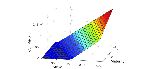
Figure 2: Price of a call option on a discount bond. The bond maturity is $5$ years. The information-adjusting function is set as $\phi(x)=\mbox{$\rm e$}^{-0.05x}$, and the initial term structure is assumed flat so that $P_{0T}=\mbox{$\rm e$}^{-0.02T}$. The information flow rate is set as $\sigma=0.25$.

Analogous calculations can be performed to obtain the price of an option on the swap rate:

$$C_{s}={\mathbb{E}}^{\mathbb{B}}\left[\left(\int_{t}^{T_{n}}\!\rho_{0}(x)\,\mbox{$\rm e$}^{\sigma\phi(x)\xi_{t}-\frac{1}{2}\sigma^{2}\phi^{2}(x)t}\mbox{$\rm d$}x-K\sum_{i=1}^{n}\int_{T_{i}}^{\infty}\!\rho_{0}(x)\,\mbox{$\rm e$}^{\sigma\phi(x)\xi_{t}-\frac{1}{2}\sigma^{2}\phi^{2}(x)t}\mbox{$\rm d$}x\right)^{+}\right].$$ (31)

The point is that the random variable $\xi_{t}$ appearing here is Gaussian with mean zero and variance $t$ in the ${\mathbb{B}}$-measure, and hence (31) reduces to merely performing a single Gaussian integration. Thus we see that in the present framework we can obtain semi-analytic pricing formulae, involving elementary Gaussian integrations, for both caplets and swaptions.

We note that the value of the parameter $\sigma$ can be calibrated from the option price (29) or (30). Whether this can always be done consistently depends on whether the option vega defined by ${\mathcal{V}}=\partial C/\partial\sigma$ changes its sign. We have considered special cases for the a priori density $\rho_{0}(x)$ and various specifications of $\phi(x)$ to confirm the positivity/negativity of ${\mathcal{V}}$, suggesting that either ${\mathcal{V}}>0$ or ${\mathcal{V}}<0$ holds for arbitrary $\rho_{0}(x)$ and monotonic $\phi(x)$. Hence it seems plausible that ‘implied volatility’ $\sigma(K)$ in the present framework can always be determined unambiguously from option prices.

7. Interpretation of the auxiliary measure. The probability measure ${\mathbb{B}}$ introduced here somewhat artificially for the purpose of calculating derivative prices in fact embodies an economic interpretation. This can be seen from the expression (14) for the bond price volatility $\Sigma_{tT}$, which shows that the $\Sigma_{tT}$ is invariant under the shift $\phi(X)\to\phi(X)+\alpha_{t}$ in the drift of the information process for any $\{\alpha_{t}\}$ independent of $X$. This degree of freedom can be used to fix the risk premium according to $\lambda_{t}=-\sigma{\hat{\Phi}}_{tt}$ without loss of generality (see also the discussion in Brody & Hughston 2002). Thus we find that the auxiliary measure ${\mathbb{B}}$ introduced for the purpose of option pricing can be identified with the market measure. It also follows that the constant initial term structure model (11) can now be seen as an example of the semilinear model introduced in Brody & Hughston (2002).

The key point to note here is that the specification of a model $\{\xi_{t}\}$ for the flow of information concerning the timing of the liquidity risk fixes both the short rate process $\{r_{t}\}$ and the risk premium process $\{\lambda_{t}\}$. As a consequence, we find that the process $\{\pi_{t}\}$ defined by the expression

$$\pi_{t}=\int_{t}^{\infty}p_{t}(x)\mbox{$\rm d$}x$$ (32)

appearing, for example, in the denominator of the bond price (8), is the pricing kernel, where $p_{t}(x)$ denotes the unnormalised conditional probability density for the random variable $X$ given ${\mathcal{F}}_{t}$:

$${\mathbb{Q}}\left(X\geq t|{\mathcal{F}}_{t}\right)=\frac{\int_{t}^{\infty}p_{t}(x)\mbox{$\rm d$}x}{\int_{0}^{\infty}p_{t}(x)\mbox{$\rm d$}x}.$$ (33)

In other words, $\{p_{t}(x)\}$ solves the Zakai equation associated with the filtering equation for $\phi(X)$. This observation is useful in considering the pricing of hybrid derivatives on account of the fact that if $H_{T}$ represents the random payout on the maturity day $T$ of a derivative contract (for example, the payoff $H_{T}=(S_{T}-K)^{+}$ of a European option on a stock), then the price $H_{tT}$ of the derivative at time $t\leq T$ is given by

$$H_{tT}=\frac{{\mathbb{E}}^{\mathbb{B}}[\pi_{T}H_{T}]}{\pi_{t}}.$$ (34)

In particular, for $H_{T}=1$ we recover the bond pricing formula. Similarly, if $\{\pi_{t}^{i}\}$ is the pricing kernel calibrated to currency $i$ and $\{\pi_{t}^{j}\}$ is the pricing kernel calibrated to currency $j$, then the arbitrage-free and friction-free foreign exchange rate is given by the ratio $\pi_{t}^{i}/\pi_{t}^{j}$. In particular, it is the market perception of the random variables $X^{i}$ and $X^{j}$ that determines the exchange-rate volatility (for a pricing-kernel approach to interest rate and foreign exchange system, see Brody & Hughston 2004 and references cited therein).

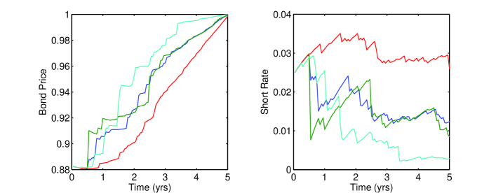
Figure 3: Sample paths of the discount function (36) and the associated short rate (37). The information-adjusting function is set as $\phi(x)=\mbox{$\rm e$}^{-0.02x}$, and the initial term structure is assumed flat so that $P_{0T}=\mbox{$\rm e$}^{-0.025T}$. The rate is set as $m=0.1$, and the bond maturity is 5 years.

It should be remarked parenthetically that although in the present investigation we have closely examined a simple model (5) for the market information, many of the derived concepts are applicable to a wide range of models for $\{{\mathcal{F}}_{t}\}$. Of course, expressions for various quantities such as the bond price or forward rate volatility are dependent on the choice of the information process. For example, if the rate at which information concerning the value of $\phi(X)$ is revealed to the market is time dependent, then the Markov information model (5) will be modified to a non-Markov process: $\xi_{t}=\phi(X)\int_{0}^{t}\sigma_{s}\mbox{$\rm d$}s+B_{t}$. The price of the bond in such a scenario can still be calculated straightforwardly, with the result

$$P_{tT}=\frac{\int_{T}^{\infty}\rho_{0}(x)\,\mbox{$\rm e$}^{\phi(x)\int_{0}^{t}\sigma_{s}{\rm d}\xi_{s}-\frac{1}{2}\phi^{2}(x)\int_{0}^{t}\sigma_{s}^{2}{\rm d}s}\mbox{$\rm d$}x}{\int_{t}^{\infty}\rho_{0}(x)\,\mbox{$\rm e$}^{\phi(x)\int_{0}^{t}\sigma_{s}{\rm d}\xi_{s}-\frac{1}{2}\phi^{2}(x)\int_{0}^{t}\sigma_{s}^{2}{\rm d}s}\mbox{$\rm d$}x}.$$ (35)

Alternatively, we may consider an interest rate model driven by pure jump Lévy processes. An example is given by the gamma filter introduced in Brody et al. (2008), whereby the information process is $\xi_{t}=X\gamma_{t}$. Here $\{\gamma_{t}\}$ denotes a standard gamma process with rate parameter $m$. In this case, the expression for the bond price process reads

$$P_{tT}=\frac{\int_{T}^{\infty}\rho_{0}(x)x^{-mt}\mbox{$\rm e$}^{-\xi_{t}/x}\mbox{$\rm d$}x}{\int_{t}^{\infty}\rho_{0}(x)x^{-mt}\mbox{$\rm e$}^{-\xi_{t}/x}\mbox{$\rm d$}x},$$ (36)

and the associated short rate process is

$$r_{t}=\frac{\rho_{0}(t)t^{-mt}\mbox{$\rm e$}^{-\xi_{t}/t}}{\int_{t}^{\infty}\rho_{0}(x)x^{-mt}\mbox{$\rm e$}^{-\xi_{t}/x}\mbox{$\rm d$}x}.$$ (37)

Hence the present framework provides for a wide range of new interest rate models to be created that are tractable and relatively easy to implement.

8. Interpretation of the function $\phi(x)$. Let us now discuss the choice of the function $\phi(x)$ introduced in the information process (5). What might appear to be the most natural candidate for $\phi(x)$ is a linear function: $\phi(x)=x$. As indicated above, in this case the bond volatility has a natural characterisation given by the difference between (17) and (16). We find, however, that in this model the market price of risk (the excess rate of return above the short rate) is strictly negative. From information-theoretic point of view, such a market can be interpreted as follows. Recall that a small value of $X$ implies that there is an acute liquidity crisis awaiting. However, according to the information process $\xi_{t}=\sigma tX+B_{t}$ there is little prior warning to the market concerning the ‘smallness’ of $X$, since $\{\xi_{t}\}$ in this case is dominated by noise. As a consequence, liquidity issues arise essentially as a surprise. What the model shows is that in such a scenario the risk premium becomes negative.

Under normal market conditions, we expect the risk premium be positive. This is obtained by a function $\phi$ such that it decreases to zero (or increases to zero if $\phi\leq 0$) for large $X$. Examples of this type are $\phi(x)=\pm\mbox{$\rm e$}^{-\kappa x}$ for a positive $\kappa$, or $\phi(x)=\pm(x-x_{0})^{-1}$ for a positive $x_{0}$. For these choices, small values of $X$ carry heavier weights in the signal component, as compared to larger values of $X$. As a consequence, signals of an imminent liquidity crisis reach the market ahead of time, enabling appropriate precautions to be taken, thus leading to a positive risk premium. This feature can be understood in conjunction with the fact that the observation $\{\xi_{t}\}$ is a Brownian motion in the market measure. The bond volatilities in these examples are determined by certain weighted annuity prices. For example, when $\phi(x)=\mbox{$\rm e$}^{-\kappa x}$ we have

$$\Sigma_{tT}=\left(\mbox{$\rm e$}^{-\kappa T}-\mbox{$\rm e$}^{-\kappa t}\right)-\kappa\left[P_{tT}^{-1}\int_{T}^{\infty}\mbox{$\rm e$}^{-\kappa x}P_{tx}\mbox{$\rm d$}x-\int_{t}^{\infty}\mbox{$\rm e$}^{-\kappa x}P_{tx}\mbox{$\rm d$}x\right].$$ (38)

It is worth remarking that the positivity of the risk premium in the arbitrage pricing theory is an assumption that cannot be deduced from the no arbitrage condition. Hence it is satisfying that in the present framework we are able to deduce how the structure of the flow of information affects the signature of the risk premium. In particular, it may be possible to use the functional degree of freedom $\phi(x)$ to calibrate various derivative prices. This is useful, because it is virtually impossible to estimate the risk premium directly from the price process of risky assets.

9. Discussion. Empirical studies indicate that a persistent increase in money supply leads in short term (up to a month or so) to a fall in nominal interest rates—this is the so-called liquidity effect (Cochrane 1989). On the other hand, in the longer term an increase in money supply increases expected inflation, hence leading to an increase in nominal rates—this is the so-called Fisher effect. Typically both effects coexist in that an increase in money supply reduces nominal rates but increases expected inflation so that the real rate also falls. Needless to say, interrelations between these effects are difficult to disentangle. The implication of these macroeconomic considerations to the present approach is that the random variable $X$, which we identified as representing the timing of liquidity crisis in the narrow sense of cash demand, is dependant on a number of market factors and not merely on money supply.

Going forward, we would like to formulate a model for real discount bonds, thus allowing us to price inflation-related products in a manner consistent with the nominal interest rate dynamics. One way of realising this within the information-based pricing framework might be through using multiple market factors (cf. Macrina 2006). This would allow inflation to be modelled consistently with the interest rate term structure.

Our objective here has been the introduction of a new interest rate modelling framework that captures some important macroeconomic elements, in such a way that resulting models can be used in practice for the pricing and risk management of interest rate derivatives. The random variable $X$, whose existence is ensured by the positivity of nominal rates and the vanishing of infinite-maturity bond prices, has the dimension of time, and hence it has been interpreted as representing the timing of future liquidity crises. It is worth emphasising that all the results established here are, of course, independent of this particular interpretation. Nevertheless, our interpretation allows us to enhance fixed-income risk management with an intuitive understanding of the model being used.

- (1) Bielecki, T. R. & Rutkowski, M. Credit Risk: Modelling, Valuation and Hedging (Berlin: Springer-Varlag 2002).
- (2) Brody, D. C. & Hughston, L. P. 2001 Interest rates and information geometry. Proceedings of the Royal Society London A457, 1343-1364.
- (3) Brody, D. C. & Hughston, L. P. 2002 Entropy and information in the interest rate term structure. Quantitative Finance 2, 70-80.
- (4) Brody, D. C. & Hughston, L. P. 2004 Chaos and coherence: a new framework for interest rate modelling. Proceedings of the Royal Society London A460, 85-110.
- (5) Brody, D. C., Hughston, L. P. & Macrina, A. 2007 Beyond hazard rates: a new framework for credit-risk modelling. In Advances in Mathematical Finance: Festschrift Volume in Honour of Dilip Madan (Basel: Birkhäuser).
- (6) Brody, D. C., Hughston, L. P. & Macrina, A. 2008 Dam rain and cumulative gain. Proceedings of the Royal Society London A464, 1801-1822.
- (7) Cochrane, J. H. 1989 The return of the liquidity effect: A study of the short-run relation between money growth and interest rates. Journal of Business and Economic Statistics 7, 75-83.
- (8) Efron, B. & Johnstone, I. M. 1990 Fisher’s information in terms of the hazard rate. Annals of Statistics 18, 38-62.
- (9) Flesaker, B. & Hughston, L. P. 1996 Positive interest. Risk Magazine September, 46-49.
- (10) Friedman, M. 1968. The role of monetary policy. American Economic Review 58, 1-17.
- (11) Hunt, P. J. & Kennedy, J. E. 2000 Financial Derivatives in Theory and Practice (Chichester: Wiley).
- (12) Macrina, A. 2006 An information-based framework for asset pricing: -factor theory and its applications. PhD thesis, King’s College London.