Effects of resolution and helium abundance in A star surface convection simulations

Abstract

We present results from 2D radiation-hydrodynamical simulations of fully compressible convection for the surface layers of A-type stars with the ANTARES code. Spectroscopic indicators for photospheric convective velocity fields show a maximum of velocities near $T_{\rm eff}\sim 8000$ K. In that range the largest values are measured for the subgroup of Am stars. Thus far, no prognostic model, neither theoretical nor numerical, is able to exactly reproduce the line profiles of sharp line A and Am stars in that temperature range. In general, the helium abundance of A stars is not known from observations. Hence, we have considered two extreme cases for our simulations: a solar helium abundance as an upper limit and zero helium abundance as a lower limit. The simulation for the helium free case is found to differ from the case with solar helium abundance by larger velocities, larger flow structures, and by a sign reversal of the flux of kinetic energy inside the hydrogen ionisation zone. Both simulations show extended shock fronts emerging from the optical surface, as well as mixing far below the region of partial ionisation of hydrogen, and vertical oscillations emerging after initial perturbations have been damped. We discuss problems related to the rapid radiative cooling at the surface of A-type stars such as resolution and efficient relaxation. The present work is considered as a step towards a systematic study of convection in A- to F-type stars, encouraged by the new data becoming available for these objects from both asteroseismological missions and from high resolution spectroscopy.

Introduction

Research on A-type has benefitted enormously from the introduction of high resolution spectrographs with $R\gtrsim 100,000$ and from advancements in asteroseismology through telescope networks and satellite missions. They provide a new way of probing our theoretical understanding of these objects and address questions such as: how are convection and pulsation linked to each other, in a physical parameter region no longer completely dominated by the strong envelope convection found in cool stars such as our Sun? How does convective mixing in these stars affect diffusion processes? What physical mechanism let chromospheres disappear in early A-type stars? How much does convection influence observed spectra and how does convection interfere with determining stellar parameters from spectroscopy? This selection of physical questions demonstrates that A stars provide a unique physical laboratory (Landstreet, 2004) underlying the richness observed in their spectra (Adelman, 2004).

In the following we report on the first results from a project on numerical simulations of A-type (and F-type) stars, motivated by the progress made by asteroseismological missions such as CoRoT and MOST and challenged by results from high resolution spectroscopy. The simulations ultimately aim at improving our understanding of the dynamical processes of convection and its interaction with pulsation and, through mixing, on diffusion processes that shape the appearance of A-type stars. We first provide a background on how convection has observationally been identified in A-type stars. We then summarise the theoretical explanations given for the peculiar convective line broadening found in A stars and review previous attempts made to model the surface convection zones in these stars. In the subsequent section we discuss the setup of the numerical simulations we have performed for mid A-type stars followed by a discussion of our results and our conclusions as well as an outlook on further work.

Observational Background

The existence of convection in the surface layers of A stars was first predicted by Siedentopf (1933). Initially, observational evidence for such convection zones came from a non-zero microturbulence parameter $\xi$. Common values for $\xi$ were found in the range of $2\dots 4$ km s^-1 for both normal A and Am-type main sequence stars (see Landstreet 2007 for a review and Adelman 2004 for examples and further references). This readily exceeds the microturbulent velocities found for their cool star counterparts (see Gray 1988 for an extended discussion of $\xi$ in cool stars). To find direct evidence for convective velocity fields in the shapes of spectral lines of A stars is much more difficult. The average projected rotational velocities of normal A-type stars is found to be $>120$ km s^-1 and even for Am stars $v_{\rm e}\sin i$ values of less than $10\dots 15$ km s^-1 are the exception and not the rule (cf. the tables and references shown in Adelman 2004 and also the recent study of Royer et al. 2007). Hence, first evidence that the bisectors of spectral lines in early type (sharp line) stars do not resemble those observed for cool stars was found for late F-type supergiants (Gray & Toner, 1986) and the early F-type bright giant Canopus (Dravins & Lind, 1984; Dravins, 1987). Stars in this parameter range were shown to feature line profiles with curved bisectors caused by extended depressions in the blue wing of spectral lines. This results in an asymmetric line shape inverted in comparison with line profiles of cool supergiants (and those of our Sun and other cool main sequence stars). First evidence for this feature to be present in main sequence A stars was reported by Gray & Nagel (1989) for the case of HR 178 (HD 3883, an Am star).

This was followed by a study of Landstreet (1998) who found two Am stars, HR 4750 (HD 108642) and 32 Aqr (HD 209625), to show large asymmetries and a depressed blue wing in profiles of strong spectral lines. Weak lines were found to have much smaller profile asymmetries or even none at all. The same effects were found to be slightly weaker in the case of the hotter A-type star HR 3383 (HD 72660). A hot A-star with similar properties, HR 6470 A (HD 157486 A), was identified by Silaj et al. (2005). The current status of observational evidence of velocity fields caused by surface convection in main sequence A stars is analysed in Landstreet et al. (2009), who added another five stars to this sample. The newly identified objects include a mid A-type star with strong line profile asymmetries as previously found only for Am stars (Gray, 1989; Landstreet, 1998). Based on the collected data, which involved also reobserving objects during the same night, in consecutive nights, in different runs, and in different wavelength ranges, they concluded that the properties of the line profiles of these stars are robust. Furthermore, they concluded that the only explanation for the line profiles which is consistent with the observational data is the presence of photospheric velocity fields not related to pulsation thus confirming the suggestion by Landstreet (1998). These velocity fields are present in both normal A and in Am stars, though the latter contain the most extreme cases, in agreement with their higher values of $\xi$. It is interesting to note that chromospheric activity indicators were identified for A-type stars with $T_{\rm eff}\lesssim 8200$ K (Simon et al., 2002) which roughly coincides with the effective temperature of those stars for which the largest profile asymmetries and overall convective line broadening have been identified (Landstreet et al., 2009).

Theoretical Explanations and Previous Simulations

The most straightforward explanation for the “inverted” or “reversed” line bisectors has already been given by Gray & Toner (1986) for the case of supergiants who suggested that this could be caused by hot columns of rising gas outshining the cold downflows. This was further developed by Gray (1989) and Dravins (1990) who noted that the hot upflows need to cover only a small fraction to reproduce such line profiles. This idea was also discussed for the case of main sequence A stars by Landstreet (1998).

Could this be recovered from non-local models of convection or radiation-hydrodynamical simulations? A first study of the coupled convection zones caused by ionization of H i (and He i) as well of He ii was presented in Latour et al. (1981), who used a modal expansion of an anelastic approximation to the hydrodynamical equations to describe convective motions in a mid A-type star. They noted the two convection zones to be coupled by overshooting. Due to the large He abundance (Y=0.354) assumed in this work it is difficult to compare it with more recent calculations (the large value of $Y$ might partially explain why they found the convective flux to be larger in the He ii ionisation zone, a property not recovered in later work). Xiong (1990) presented solutions obtained from his non-local model of convection for an F-type, an A-type, and two late B-type stars. Two separate convection zones were found coupled by overshooting for the mid A-type star with a convective flux being larger for the photospheric convection zone. A solar He abundance (Y=0.28) was assumed, as in the study of Kupka & Montgomery (2002), who used the fully non-local convection model of Canuto & Dubovikov (1998) and Canuto et al. (2001) to construct envelopes of A stars for an evolutionary sequence of a 2.1 $M_{\odot}$ star and for an effective temperature sequence at three different metallicities. Except for the hottest A stars the two convection zones were found to be coupled by overshooting with the photospheric zone dominating in mid and late A-type stars (in agreement with the numerical simulations by Freytag 1995, see below). They also investigated photospheric overshooting and found a positive kinetic energy flux for the observable layers of mid and late A-type stars. Such a distribution agrees with the model of Gray (1989); Dravins (1990); Landstreet (1998), although no synthetic spectra were computed at that point.

The first radiation-hydrodynamical (RHD) simulations of a mid A-type star in two spatial dimensions (2D) with $49\times 42$ grid points were presented in Sofia & Chan (1984) (radial resp. vertical coordinate listed first here and in the following). However, an impenetrable upper boundary condition had to be placed at optical depths $\tau$ of 0.22 to $2/3$ in those simulations. This put the boundary layer right into the zone of partial ionisation of H i with its accompanying density inversion and pushed vertical velocities to zero in that layer. Consequently, the lower convection zone due to ionisation of He ii was found to dominate even at a solar He abundance and no predictions of photospheric velocities could be made. The stably stratified layers in-between those two zones were found to be fully mixed. In Gigas (1989) a 2D RHD simulation for the parameters of Vega was presented. The model had $30\times 36$ points, but extended to much lower optical depths of $\log\tau\sim-2.4$. No He ionisation was included in the equation of state and simulation time had to be limited to one hour of stellar time. Vertical oscillations were found in the photosphere instead of a pattern of up- and downflows. Interestingly, line profiles calculated using that simulation were found to be bent bluewards. However, a comparison with Landstreet (1998) reveals that although the resulting bisector looks similar to those found for strong lines in HD  72660, a strong asymmetry is also found for weak lines contrary to observations, as corroborated by the analysis of Landstreet et al. (2009), who included another four stars in that $T_{\rm eff}$ range of 8900 K to 10000 K in their analysis. Given the short simulation time and the reported periods of 5 to 15 min the observed oscillations could also have been transient. This is also implied by results of the first extended study of A stars by means of 2D RHD simulations by Freytag (1995) (see also Freytag et al. 1996), who found oscillations to be damped even for a $T_{\rm eff}\sim 9000~{}K$ and a $\log(g)=3.9$, i.e., at the blue edge of the $\delta$ Sct instability strip, while oscillations were clearly excited in an even cooler model. Most of the simulation in Freytag (1995) were carried out for a typical resolution of $65\times 62$ grid points, with a few simulations doubling horizontal resolution, and one case reaching $95\times 182$ points for a short run. A solar chemical composition was assumed throughout and partial ionisation was accounted for as well. The case of non-grey radiative transfer was considered for one model and found to have little influence on the model structure and the flow itself. The convective (enthalpy) flux was always found to be larger in the H i driven convection zone compared to the deeper one driven by He ii (if included in the simulation box) for models with $T_{\rm eff}\lesssim 9000~{}K$ with the two convection zones always connected by overshooting. A characteristic property of the simulations were nevertheless rather high velocities in the lower convection zone with vertical root mean square ($v_{\rm rms}$) maxima often around 1 km s^-1. These maxima are related to strong vortices found in the lower convection zone. No synthetic spectra were computed from those simulations.

A surprising change to these developments came finally with the first RHD simulations in 3D for two mid A-type main sequence stars by Freytag & Steffen (2004) (with a $T_{\rm eff}$ of 8000 K and 8500 K for a $\log(g)$ of 4.4). The grey approximation and a solar chemical composition were assumed. 90 to 110 grid points were used along the vertical direction and 180 points along the horizontal ones. Similar to the previous 2D RHD simulations and solar granulation simulations they followed a box-in-a-star approach in which a limited volume located near the surface of the star is considered for the calculations. Contrary to most of the preceding 2D simulations the extent of the simulation boxes considered by Freytag & Steffen (2004) were chosen such as to contain at least several up- and downflow structures along any horizontal direction, which explains the larger number of grid points. Nevertheless, their simulations revealed the usual granulation pattern, with some subtle differences. In the end this lead to line profiles very much looking like solar ones in contradiction to the observations by Landstreet (1998). The calculated line profiles were further analysed by Steffen et al. (2006). In a follow-up work a third 3D RHD simulation (for a $T_{\rm eff}$ of 8000 K and a $\log(g)$ of 4.0) was presented by Kochukhov et al. (2007) using again the CO⁵BOLD code as in Freytag & Steffen (2004) and Steffen et al. (2006), but this time with a slightly higher resolution ($170\times 220^{2}$). In addition, part of the run was repeated using non-grey radiative transfer (based on binned opacities). Due to the latter the match for weak lines of stars such as HD 108642 (with actual stellar abundances used for the spectrum synthesis) improved. The same held for the cores of strong lines, but the wings of strong lines remained clearly discrepant both in shape, width, and bisector curvature. Only one more 3D RHD simulation of a cool A-star ($T_{\rm eff}=7300$ K, $\log(g)=4.3$, solar metallicity, non-grey) with $82\times 100^{2}$ grid points was presented in more detail by Trampedach (2004), though without computations of stellar spectra. However, in that simulation the H i and He ii zones are still connected to a single layer in a configuration described to be highly unstable. Further work in the literature has dealt with simulating interacting convection zones assuming idealised microphysics, but these results cannot be directly compared to stellar observations without invoking additional assumptions on the surface radiative cooling and the effects of chemical composition.

The discrepancy found by Freytag & Steffen (2004) is surprising, since RHD simulations using the same code had been used to compute realistic solar spectra that match observed line profiles (see Steffen 2007 and references therein). Obviously, the simulation results are in contradiction with the model of hot and narrow, rapidly rising columns of gas. The observations discussed by Landstreet et al. (2009) indicate that chemical peculiarity (Freytag & Steffen, 2004) can play only a limited role, as the line profile anomaly is found in both Am and normal A stars. This still cannot exclude He abundance to play a role (Kupka, 2005), at least at the level of explaining the differences between stars showing the most asymmetric and broadened profiles (of Am-type) and their counterparts among normal A stars. Effects of rotation might have to be considered, too (suggested by Arlt in Freytag & Steffen 2004, some consequences were analysed in Kupka 2005). This suggestion was also motivated by the frequent binary nature of the observed sharp line stars. However, the line profiles in Landstreet (1998) and Landstreet et al. (2009) do not resemble at all the flat-bottomed line profiles of rapid rotators seen pole-on such as Vega (Gulliver et al., 1994; Hill et al., 2004). Since there is no indication from the data on the sample of Landstreet et al. (2009) that the binaries are very close or interacting, nor that there is any dependence of the profiles on the rotation period other than the ability of detecting them, rotation appears to be a less likely candidate to resolve this discrepancy. Rather, numerical resolution (Freytag & Steffen, 2004) or the entire scheme used for the radiative transfer (Landstreet, priv. comm. 2004) may play a much more important role (see also Kupka 2005).

Numerical Simulations of A-type Stars with ANTARES

To investigate the cause of these discrepancies between observation and numerical simulations we have decided to perform RHD simulations of A-type stars with the ANTARES code (Muthsam et al. 2007, Muthsam et al. 2009). This work is part of a more extended research project on convection in A- and F-type stars intended to study convection-pulsation interaction and the properties of convection under physical conditions that lead to very different efficiencies for the transport of heat and for the mixing of fluid, respectively.

As a first step we decided to have a closer look at the effects of helium abundance and of resolution, since both have not been investigated yet in sufficient detail. In addition, we also wanted to clarify the nature of the extremely restrictive time steps due to the short radiative cooling time scale $t_{\rm rad}$ (Freytag & Steffen, 2004; Steffen, 2007) (see Eq. (5)). As ANTARES currently solves the fully compressible equations of hydrodynamics coupled to the stationary radiative transfer equation with a fully explicit time integration method, the ensuing time step constraints due to $t_{\rm rad}$ are severe and the resulting computational costs very high (10 to 100 times higher than for a solar granulation simulation of comparable resolution according to Freytag & Steffen 2004). We have thus begun our study with RHD simulations in 2D to single out the most promising cases for 3D simulations and possibly suggest improvements to the time integration to reduce the computational costs of 3D simulations.

With ANTARES we solve the RHD equations for fully compressible flows,

$$\frac{\partial\rho}{\partial t}+\nabla\cdot\left[\rho{\bf u}\right]=0,$$ (1)

$$\frac{\partial\rho{\bf u}}{\partial t}+\nabla\cdot[\rho{\bf u}{\bf u}+p\underline{I}]=\rho{\bf g}+\nabla\cdot\underline{\tau},$$ (2)

$$\frac{\partial e}{\partial t}+\nabla\cdot[{\bf u}(e+p)]=\rho({\bf g}\cdot{\bf u})+\nabla\cdot({\bf u}\cdot\underline{\tau})+Q_{\rm{rad}},$$ (3)

which are the continuity, Navier-Stokes, and total energy equation describing the conservation of mass density $\rho$, momentum density $\rho{\bf u}$, and total energy density $e$. The later is the sum of internal ($e_{\rm int}$) and kinetic energy density, respectively, and ${\bf u}$ is the flow velocity. An equation of state (EOS) relates $e_{\rm int}$ and $\rho$ to the temperature $T$ and the gas pressure $p$ (or rather, the sum of gas pressure and isotropic radiation pressure $p_{\rm rad}$, the meaning of $p$ as used in the following). The EOS is taken from the most up-to-date OPAL tables (Rogers et al., 1996) and used also to compute all other required thermodynamic derivatives. We note that $\underline{I}$ is simply the identity matrix, $\underline{\tau}$ is the viscous stress tensor, and $t$ and ${\bf x}$ denote time and space. The simulations discussed below are box-in-a-star simulations for a limited volume ranging from the upper photosphere to the stably stratified layers around $T\sim 60,000$ K to $70,000$ K, thus containing the surface convection zones inside the box. Since this region is small with respect to the stellar radius, a Cartesian (box) geometry is taken for the simulation box and the gravity ${\bf g}$ is a constant, downwards pointing vector equalling the surface gravity $g$. Horizontal boundary conditions are hence periodic and the geometry is plane parallel. The horizontal domain is chosen wide enough to fit several up- and downflow structures into the box at photospheric depth. The vertical boundary conditions are assumed to be impenetrable and stress-free (free-slip) with a constant energy flux assumed at the bottom of the simulation zone (and directly related to the $T_{\rm eff}$ defined for the simulation). The lower boundary is placed sufficiently far below the convection zones to have only limited influence (at most through reflecting waves). The upper boundary condition is placed at $\log\tau_{\rm ross}\sim-5$ for similar reasons. The appropriate domain sizes are estimated from scaling the linear dimensions of solar granulation simulations by the pressure scale height $l=H_{p}=P/(\rho g)\sim T/(\mu g)$, which when comparing to the Sun implies

$$l/l_{\odot}=T_{\rm eff}\mu_{\odot}g_{\odot}/(T_{\rm eff,\odot}\mu g)$$ (4)

for a star characterised by $(T_{\rm eff},\mu,g)$, where $\mu$ is the mean molecular weight. In optically thick layers the radiative (heating and) cooling rate $Q_{\rm rad}=\nabla\cdot F_{\rm rad}$ can be computed from the diffusion approximation $F_{\rm rad}=-K_{\rm rad}\nabla T$, where $K_{\rm rad}$ is the radiative conductivity obtained from equation of state quantities and the Rosseland opacity $\kappa_{\rm ross}$. For the latter, we use tabulated OPAL opacities (Iglesias & Rogers, 1996) extended at low temperatures with tables by Ferguson et al. (2005), both computed for the solar mixture of Grevesse & Noels (1993). For the photospheric layers a radiative transfer equation must be solved for accurate computation of $Q_{\rm rad}$. This computation is extended into deeper layers to allow a smooth transition to the diffusion approximation. Details on this procedure as used in ANTARES are given in Obertscheider (2007) and in Muthsam et al. (2009). We note that even in the grey approximation the results of this approach are different from the plain diffusion approximation. In ANTARES the stationary limit of the radiative transfer (intensity) equation is assumed (as in Freytag 1995, Freytag & Steffen 2004, Kochukhov et al. 2007) and the resulting $Q_{\rm rad}$ is computed from an integration of the intensity obtained for a finite set of rays from this procedure. The grey case differs from the non-grey one by just integrating along each ray for a single frequency band rather than for multiple ones, but contrary to the diffusion approximation this accounts for inhomogeneity of cooling and heating in a convective stellar photosphere. We also point out here that the assumption of stationarity (instantaneous radiative transfer) leaves $\rho$, $\rho{\bf u}$, and $e$ as the dynamical variables of the system which have to be followed by the time integration during the simulation.

To perform simulations which are close to an observational case we have chosen $T_{\rm eff}=8200$ K and a $\log(g)=4.0$ as basic physical parameters, as they are representative of HD 108642 (Kupka et al. 2004; note that Landstreet 1998 and Landstreet et al. 2009 suggested a $T_{\rm eff}$ 100 K lower and a $\log(g)$ 0.1 dex higher than those values, but such differences are well within the observational uncertainties). Since diffusion has been suggested to substantially change the helium content of the upper envelope during the main sequence life time of A-type stars (Vauclair et al., 1974; Richard et al., 2001; Michaud, 2004), we consider two extreme cases of helium abundance: a solar one and no helium at all. A solar metallicity mass fraction of $Z=0.02$ was taken in both cases (this value is a compromise, because the underabundance of light elements relative to their solar values lowers the absolute value of $Z$ while the opacity resulting from the different chemical composition contributing to $Z$ is increased in the photosphere of Am-type stars; see Kupka et al. 2004 for further details on the abundances of HD 108642). The hydrogen mass fraction $X$ is scaled up from 0.7 to 0.98 in the case where helium is absent ($Y=0$).

For the simulations presented here we have chosen a coarse grid with a single refinement zone embedded inside the domain covered by the coarse grid. Since the simulations are in 2D, the horizontal boundary conditions of the coarse grid are periodic and because the fine grid is used to improve resolution near the surface, it has the same horizontal extent as the coarse one. Hence, it has periodic boundary conditions as well. Vertically, the fine grid is located in the interior of the coarse grid which provides the vertical boundary conditions for the fine grid. The coarse grid itself has the closed vertical boundary conditions already described above. For the case with solar helium abundance, the coarse grid has $150\times 200$ points which span a domain of $32.2\times 40.3$ Mm² and yield a resolution of $216\times 201$ km². The fine grid has $205\times 200$ points and is located vertically between about 1.1 Mm and 12.1 Mm as measured from the top of the simulation box. This provides a resolution of $54\times 201$ km², i.e., a vertical refinement by a factor of 4. For the plots shown below the vertical axis is shifted by $-3.8$ Mm to have the downwards pointing vertical axis be labelled with zero where the horizontally and temporally averaged temperature equals $T_{\rm eff}$. For the simulation without helium, a coarse grid of $130\times 210$ points is used spanning a domain of $26.1\times 41.7$ Mm² and thus providing a mesh size of $202\times 199$ km². The fine grid is located vertically between about $1.8$ Mm and $13.1$ Mm as measured from the top and has $225\times 210$ grid points. Hence, the resolution on the fine grid is $51\times 199$ km², which again implies a vertical refinement by a factor of 4. For this simulation the vertical axis is shifted in the plots shown below by $-4.6$ Mm. As a result, in plots showing both simulations the vertical axis value of zero indicates the average location where $T=T_{\rm eff}$, i.e., the optical surface, for both cases. For the radiative transfer, we have used 12 rays and a single bin for Rosseland mean opacities, i.e., the grey approximation.

Apart from setting up the simulations and some test runs which were done on single and two CPU core configurations most of the simulation runs to evolve both the solar helium and the helium-free case were done on 8 CPU cores using the MPI capabilities of ANTARES. The code was slightly modified to allow grid refinement zones to cover the entire horizontal extent of the model, as the fine grid was previously used to have higher resolution only in a specific domain of interest (cf. Muthsam et al. 2007). These enhanced possibilities to use fine grids are now a standard feature of the code (Muthsam et al., 2009). Another improvement added to the code and motivated by simulations of A-type stars was its ability to work with arbitrary chemical compositions (and thus combinations of $X$,$Y$, and $Z$), since the opacity and equation of state tables used have some restrictions on the combinations of these parameters. The improved microphysics interface is now also a standard module of the code. After initializing the simulations, all production runs were performed on the POWER5 p575 of the RZG in Garching. The initial conditions for the simulations were taken from 1D models for HD 108642 calculated with the LLmodels code (Shulyak et al., 2004) using the convection model by Canuto & Mazzitelli (1991) and opacity distribution function tables by Kurucz (1993a) and Kurucz (1993b). For the 1D models $\xi=4$ km s^-1 was assumed (Landstreet, 1998; Kupka et al., 2004) and $T_{\rm eff}$ and $\log(g)$ were the same as in the simulations (values taken from Kupka et al. 2004). The flow in the simulations is started by a lack of perfect hydrostatic equilibrium of the stratification introduced by the differences in the equation of state and opacities used, the change in grid spacing between the 1D model and the simulation, and the different numerical methods used in both codes. In addition, we add a small perturbation in the mass density field by creating a random distribution for the density perturbations in Fourier space. The values of this smooth noise function are added at each point to the average for the horizontal layer as obtained from the 1D model. The noise is equally distributed over all modes (wave numbers), but its magnitude is scaled as a function of depth to produce the largest density fluctuations where the 1D convection model predicts the largest temperature fluctuations. This avoids the introduction of long-lived perturbations in the radiative region near the bottom of the simulation box, which would cause unnecessarily long relaxation times (we return to this topic further below).

Results

In the following we discuss the main results of our 2D RHD simulations for both the case with solar helium abundance and for the case with zero helium abundance. Some results from experimental runs with different initial conditions and resolution but otherwise identical parameters are included as well.

Relaxation and oscillations

Figure 1: Vertical (solid line) and horizontal (dashes) velocities of the centre of gravity for the simulation with solar helium abundance as a function of time. The horizontal component is magnified by a factor of $10^{3}$. On the top x-axis, time is normalised by the sound-crossing time. Arrows indicate the beginning and the end of the artificial damping phase.

Both simulations were run for several sound-crossing times until convective motions had sufficiently developed, which is indicated by a growth in vorticity and in total kinetic energy. For the simulation with solar He abundance notable growth of convective motions occurred after about three sound-crossing times (time for a sound wave to cross the entire simulation box vertically, here $t_{\rm sc}=1371.6$ s). After $t/t_{\rm sc}\gtrsim 5$ convective motions dominated the contributions to kinetic energy and experienced a phase of exponential growth. Figure 1 shows the velocity of the centre of gravity of the entire simulation volume as a function of time. The oscillations triggered by the stratification being out of perfect hydrostatic equilibrium are prominent and are almost purely vertical since the horizontal component is totally negligible. There is only weak intrinsic damping. We attribute this to the quality of the advection scheme implemented in ANTARES. We removed these oscillations by introducing a damping term at $t/t_{\rm sc}\sim 6.1$ for the vertical velocity component, as is routinely done so during relaxation of solar granulation simulations (Trampedach, 1997). Due to the short time scale chosen the oscillations are rapidly damped which allows us to turn off this artificial damping after $t/t_{\rm sc}\sim 7.9$. At this point the vertical oscillations contribute $\lesssim 3\%$ to the total kinetic energy of the flow and shortly afterwards the total kinetic energy starts dropping for the first time after its rapid phase of growth and at least the upper convection zone itself is essentially relaxed. The snapshots in Figs. 5,  7, and 8 have hence been taken at $t/t_{\rm sc}\gtrsim 8$. The equivalent holds for the averages in Fig. 3 and 4.

An alternative way of visualizing vertical oscillations is to look at the motion of the photosphere and define the velocity $v_{\rm ph}$ as the horizontally averaged vertical motion of the layer for which $T=T_{\rm eff}$ (the photospheric radius) at a given point in time. For both simulations this velocity is about an order of magnitude larger than that of the centre of gravity. Figure 2 shows the time development of $v_{\rm ph}$ for the simulation with zero helium abundance. Intrinsic damping is just slightly more efficient than in the previous case. Artificial damping of vertical motions is applied from $t/t_{\rm sc}\sim 4.4$ to $t/t_{\rm sc}\sim 13.9$ onwards (here, $t_{\rm sc}=1150.9$ s). As we have used a smaller damping rate for this second simulation the damping phase is longer and smoother than for the previous case. The development of convection also takes longer: strong convective motions set in only after $t/t_{\rm sc}\sim 7$ and they dominate over the vertical oscillations in terms of kinetic energy after $t/t_{\rm sc}\sim 9$. While the convective motions increase in strength, the contributions by oscillations drop until they reach a level of $\lesssim 3\%$ at $t/t_{\rm sc}\sim 14$. Once the flow can evolve undamped, some oscillatory motions seem to rise again. This is more obvious for $v_{\rm ph}$ than for the centre of gravity, despite $v_{\rm ph}$ is also much more influenced by events taking place at the surface such as the formation of shock fronts, which contribute to the non-sinusoidal shape of the function visible in Fig. 2. With kinetic energy increasing no longer exponentially the simulation slowly reaches equilibrium at $t/t_{\rm sc}\sim 18$. The snapshot in Fig. 6 and the averages in Fig. 4 have been computed for $t/t_{\rm sc}\gtrsim 17$.

Figure 2: Temporal evolution of photospheric velocity for the simulation with zero helium abundance. On the top x-axis time is normalised by the sound-crossing time. Arrows indicate the beginning and the end of the artificial damping phase.

We notice that a proper choice of the initial perturbations is more important for simulations of surface convection in A stars than for solar granulation simulations. An earlier model for the case of solar helium abundance, which had been perturbed with an additional, sinusoidal velocity field instead of a random perturbation in density, showed strong resiliency to “forget” this pattern in the zone of He ii ionisation even after several sound-crossing times. That simulation run was hence discarded. This behaviour is quite different from the solar case where the same kind of perturbation is rapidly removed by the convective flow, for instance, in the simulations of Obertscheider (2007).

Structure of the convection zone

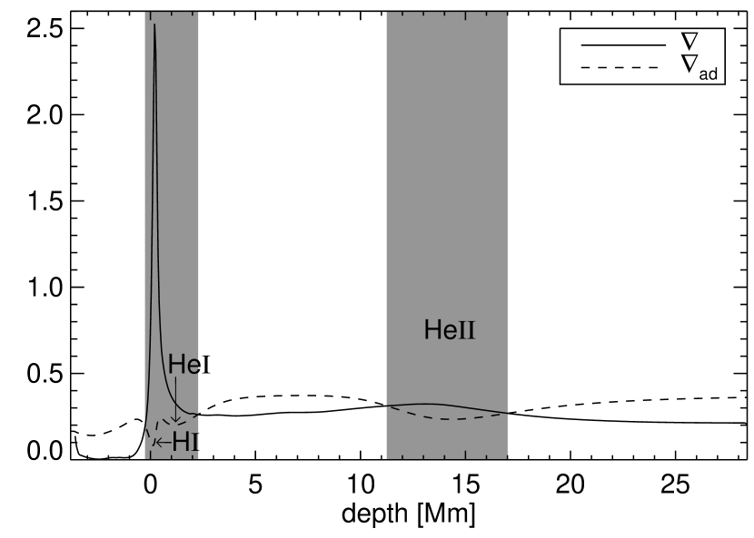
Figure 3: Temporal and horizontal average of actual ($\nabla$) and adiabatic ($\nabla_{\rm ad}$) temperature gradient for the simulation with solar helium abundance. The regions of partial ionisation of H i, He i, and He ii are indicated. Layers unstable according to the Schwarzschild criterion are indicated in grey.

In Figure 3 we show the dimensionless temperature gradient $\nabla$ and the dimensionless adiabatic gradient $\nabla_{\rm ad}$ for the simulation with solar helium abundance. The superadiabatic peak in the zone of partial hydrogen ionisation is about 3.5 times steeper than in a simulation of solar granulation (cf. Rosenthal et al. 1999 for the latter). The upper convection zone is about 2.52 Mm deep as obtained from the definition of the Schwarzschild criterion applied to the horizontally and time averaged gradients. The upper zone is mostly driven by the partial ionisation of H i. It is extended due to the partial ionisation of He i which takes place close enough to unite both regions into a single convection zone. With 5.7 Mm the second convection zone, which is caused by partial ionisation of He ii, is much larger in vertical extent. This is mostly due to the increase of the local pressure scale height. The resulting mean structure is very similar to that one found in one dimensional models of stellar atmospheres and stellar envelopes for that part of the HR diagram (cf. Vauclair et al. 1974, Latour et al. 1981, Landstreet 1998), because the high radiative losses of convection keep the stratification of the entire envelope in these stars close to that one of a purely radiative model (this has also been found by Freytag 1995, Freytag et al. 1996, Kupka & Montgomery 2002, Freytag & Steffen 2004).

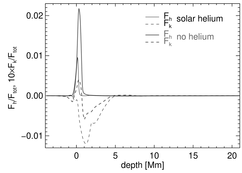
Figure 4: Convective (enthalpy) and kinetic energy flux in units of the total flux, shown as solid and dashed line, respectively, for the simulation with solar helium abundance (black thin) and without helium (grey thick). The kinetic energy flux is multiplied by a factor of 10 for better visibility.

By comparison, the simulation with zero helium abundance has just a single convection zone due to the partial ionisation of H i. Its extent into the photosphere up from where on average $T=T_{\rm eff}$ is marginally smaller than in the previous case (0.23 Mm instead of 0.25 Mm). With a total extent of 1.56 Mm when following the same definition as used above, it is more shallow than its counterpart containing helium, in spite of a larger local scale height due to a lower $\mu$, Eq. (4). This is a direct result of the lack of He i ionisation extending the zone deeper inside (note the behaviour of $\nabla_{\rm ad}$ in Fig. 3). However, with a maximum of 1.6 the gradient $\nabla$ itself is flatter and the resulting superadiabatic gradient is only about 2.3 times steeper than in solar granulation simulations.

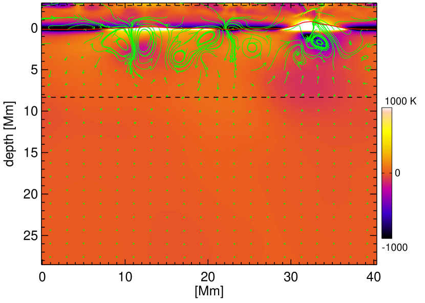
Figure 5: Snapshot of temperature fluctuations ($[T^{\prime}]=K$) relative to their horizontal mean for the simulation with solar helium abundance. Extreme values have been chopped for easier visualization. The two black dashed lines indicate the region where grid refinement has been applied. The $\tau_{\rm ross}=1$ ‘isosurface’ is denoted by a solid line. Streamlines indicate the direction and magnitude of the local flow field (the mean vertical velocity has been subtracted to improve visibility of the weakest vortices).

Differences are also visible in the flux distribution. Figure 4 displays the enthalpy (convective) flux $F_{\rm h}$ and the flux of kinetic energy $F_{\rm k}$ for both simulations in units of the total (input) flux after subtracting the contribution due to the mean flow (i.e., due to the remaining vertical oscillations). That contribution is negligible for $F_{\rm k}$, but can contribute a relative flux of up to 0.5% to $F_{\rm h}$, if the averaging time is short, i.e., $t<t_{\rm sc}$. The higher enthalpy flux found in the simulation with no helium is hardly significant since it could be the signature either of a more relaxed simulation or of an effectively stronger convection due to a lower mean molecular weight. The same could hold for the higher velocities found for the helium free case, though we consider them more likely to be caused indeed by a lower $\mu$. Nevertheless, and interestingly enough, we note that in the simulation with no helium $F_{\rm k}$ has the opposite sign for the upper half of the convection zone. This feature remains robust even when averaging for $t/t_{\rm sc}\sim 3$ and also when averaging over one third of that time scale for different subintervals. This inversion in the sign of $F_{\rm k}$, which does not appear in simulations of solar convection, occurs in our simulation with the most shallow convective zone. In this case with a really thin convective layer heating from below and cooling from above act at the same time within a pressure scale height, while in a thicker zone, such as in the model with solar helium abundance, heating and cooling are more disconnected (cf. Moeng & Rotunno 1990 for a discussion of heating from below and cooling from above in a meteorological context). We also note that at the chosen scale the fluxes in the He ii ionisation zone are not visible (cf. Steffen et al. 2006 and Steffen 2007). These small fluxes require a more careful inspection of the simulation.

Indeed, if we look at Fig. 5 we see that the strongest vortices created by the flow are located in the upper convection zone or just slightly underneath it and thus are close to the region of the strongest convective driving. The large downdraft at a horizontal coordinate of 23 Mm manages to penetrate just a little bit into the lower convection zone, but at that time no strong vortices have developed in that region. We recall our previous observation that if vortices are seeded there as an initial condition, for instance by a sinusoidal perturbation, they remain there for a long time. This is both due to the weak convective driving (which cannot rapidly destroy a vortex or push it into a stably stratified layer) and due to the general longevity of vortex patches in 2D (cf. Muthsam et al. 2007). Temperature fluctuations are found largest at the optical surface (the extrema have been truncated in the plot for a better contrast and can be four to five times larger while root mean square fluctuations are twice as large). The optical surface is corrugated mostly around rapidly evolving upflow regions.

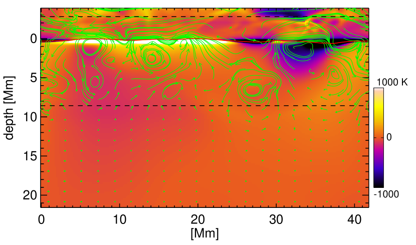
Figure 6: Snapshot of temperature fluctuations ($[T^{\prime}]=K$) relative to their horizontal mean for the simulation without helium. Scaling of $T^{\prime}$, domain boundaries of the grid refinement zone, the location of the optical surface defined at $\tau_{\rm ross}=1$, and the local velocity field (with mean vertical velocity subtracted) are indicated as in Fig. 5.

In Figure 6 we see quite a similar overall pattern for the simulation without helium. The horizontal scales are somewhat larger as expected from Eq. (4). Vortex patches are also strongest inside the convection zone itself, but a larger number of them is found further below than in Fig. 5. We think that this is a result of the longer time evolution of this simulation. Eventually, also in Fig. 5 downflows from above will form new vortex patches in the lower convection zone or patches located in the stably stratified layer in between will reach it. Thus, if we run the simulation with solar helium abundance significantly longer, we may eventually see an increase in $F_{\rm h}$. However, this may not be more realistic, as the vortex patches in 2D just happen to assemble near the bottom of a simulation of a strongly stratified medium (cf. Muthsam et al. 2007). Since 3D simulations started from 2D ones may inherit these properties for quite some (simulation) time, we think that future long-term simulations are the only way to accurately compute the enthalpy and kinetic energy fluxes in the lower convection zone of models for A stars with a helium content large enough to drive that zone.

Shock fronts and their development

As we can conclude from the small enthalpy fluxes found for both simulations shown in Fig. 4 convection is rather inefficient in transporting heat in mid A-type stars, a result also reported by Freytag (1995), Freytag et al. (1996), Kupka & Montgomery (2002), Freytag & Steffen (2004), Steffen et al. (2006), and Steffen (2007). Consequently, the mean temperature gradient stays close to the radiative one and hence, contrary to RHD simulations of solar granulation, a density inversion appears in the layer where H i is partially ionised (Freytag, 1995). This is a consequence of the lower mean molecular weight which in turn is caused by the doubling of the number of particles contributed by ionised hydrogen relative to neutral one. In the Sun efficient convection and thus a much flatter $\nabla$ is counterbalancing this effect of partial ionisation (cf. the simulations of M. Steffen and F.J. Robinson compared in Kupka 2009; the model by Canuto & Mazzitelli 1991 is an exception, since it predicts inefficient convection for the photospheric layers of the Sun which are located on top of a rapid transition to efficient, adiabatic convection dominating the bulk part of the convective envelope). Figure 7 shows a snapshot for our simulation with solar helium abundance. The density inversion is prominent and the ensuing Rayleigh-Taylor instability enhances the convective instability caused by high opacity and a low $\nabla_{\rm ad}$ (see Fig. 3 for the latter).

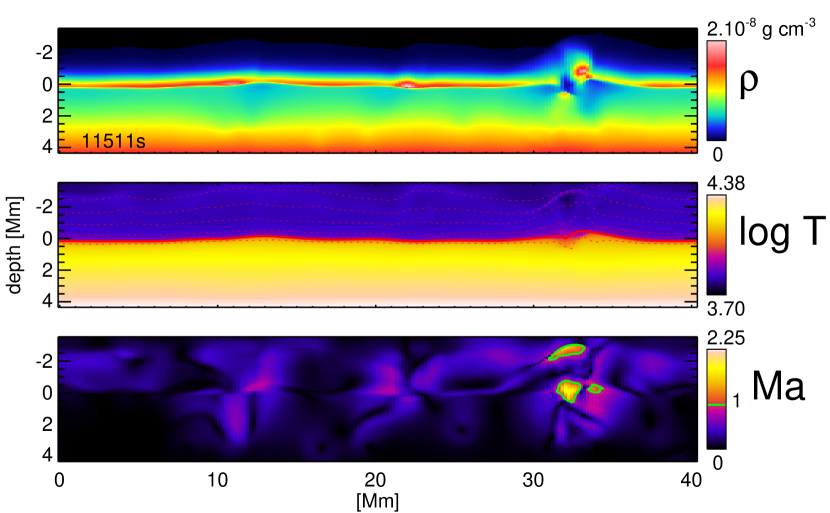
Figure 7: Mass density $\rho$, logarithm of temperature $T$ ($[T]=K$), and local Mach number in the simulation with solar helium abundance prior to the formation of a large shock front. The isoline for which $\tau_{\rm ross}=1$ is denoted in the middle panel by a thick solid line. Isolines for $\log\tau_{\rm ross}=-4,-3,-2,-1,+1$ are denoted as dotted lines. Note the density inversion near the optical surface in the top panel. Regions of supersonic flow are surrounded by a bright solid isoline where ${\rm Ma}=1$.

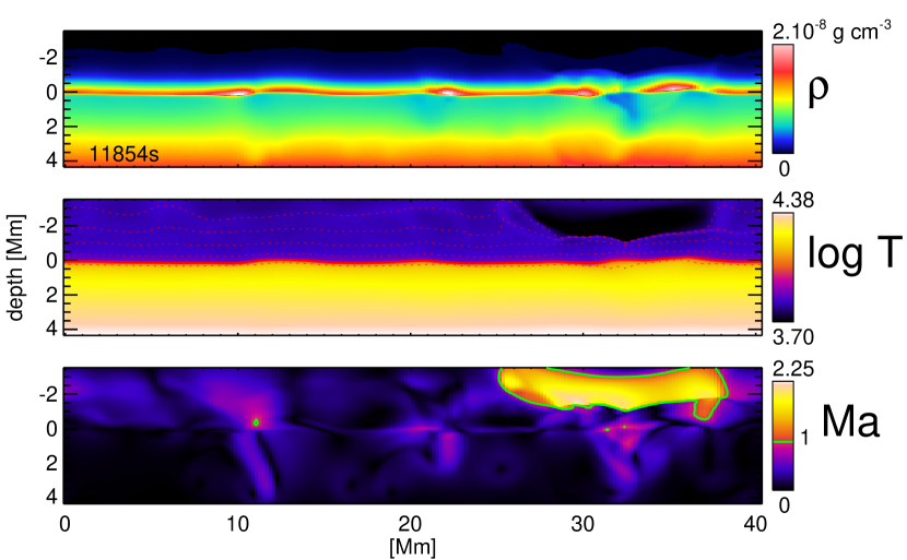
Figure 8: Mass density $\rho$, logarithm of temperature $T$ ($[T]=K$), and local Mach number in the simulation with solar helium abundance 343 s ($0.25\,t_{\rm sc}$) after the time step displayed in Fig. 7. Note the large shock front in the photosphere spreading more than $1/3$ of this layer within the simulation box. It is characterised by large jump in temperature and a relative increase in the optical depth by more than an a factor of 10. Isolines have the same meaning as in Fig. 7.

Note that the inversion layer is interrupted by a complex feature at a horizontal coordinate of $\sim 33$ Mm. In this region the optical surface is more corrugated (solid line in the temperature plot in the middle panel) and supersonic velocities are found there, too (bottom panel). This feature is the result of two counterrotating vortices, which form at some time $t/t_{\rm sc}\gtrsim 7.5$. At $t/t_{\rm sc}\sim 8$ they have created an extended region just underneath the photosphere with a temperature lower than its horizontal average. The low temperature fluid is supplied by the strong downdraft between the vortex pair which reaches supersonic velocities in its inflow area within the photosphere. At $t/t_{\rm sc}\sim 8.2$ hot gas from the neighbouring upflows has mostly covered the cold downflow region leaving a dense spot of cold material in its centre. As a result supersonic flow appears both in the two photospheric inflow areas and in the downdraft itself. From now on the structure begins to collapse emitting a series of shock fronts. At $t/t_{\rm sc}\sim 8.4$, which is shown in Fig. 7, there are no more supersonic inflow regions. Rather, supersonic velocities are found in a small front in the upper photosphere (bottom panel), visible also in $T$ (band structure trailed by material of lower $T$ underneath) and in $T^{\prime}$ in Fig. 5, which shows the state of the simulation 68 s before that one illustrated in Fig. 7. The streamlines in Fig. 5 also demonstrate that the structure is no longer dominated by a pair of roughly equally strong vortices. Supersonic flow is also found just underneath the patch of dense gas extending into the photosphere (Fig. 7).

Once this gas patch has bumped onto the layers just below it, a large shock front is created which horizontally extends over one third of the simulation box and also spreads over almost one third of the photosphere contained in the simulation volume. This can be seen in Fig. 8, at $\sim 0.25\,t_{\rm sc}$ after the state shown in Fig. 7. The snapshot shows the moment when the remainders of the previous front, which is shown still moving upwards in Fig. 7 and is reflected by the upper boundary condition shortly afterwards, are absorbed by the new front. This explains the extended high Ma number region preceding the new front (we recall here that a shock front is a (near) discontinuity in the hydrodynamic variables, which does not necessarily have to move at supersonic velocities). As the upwards moving material has much higher density, it immediately absorbs the downwards moving one with very little changes to its physical state. Note that the shock front is optically thin, although with a steep gradient in optical depth (isolines of $\log\tau_{\rm ross}=-3$ and $-4$ nearly merging with each other). At the same time the anomaly in the density stratification has nearly disappeared. Comparing with Fig. 7 we can see that the density in this region has dropped dramatically (in fact to average horizontal values) leaving a low temperature region which is reheated by the upwards moving shock front. We note that similar events also appear in the simulation run without helium and smaller events appear more frequently than the extreme case illustrated by Fig. 7 and Fig. 8. These violent events have no counterpart in simulations of solar convection performed with the ANTARES code (Muthsam et al., 2007). Even though they are intermittent in nature, they are common enough (cf. the front visible in Fig. 6 in the upper right corner of the simulation volume) to be important statistically. They may even contribute to the shape of line profiles and provide an efficient source of heating up a chromosphere (cf. Simon et al. 2002).

Resolution and computation of the radiative cooling rate $Q_{\rm rad}$

Already for the case of solar granulation the most difficult quantity to resolve in equations (1)–(3) is the radiative heating and cooling rate $Q_{\rm rad}$ (Nordlund & Stein, 1991). It directly influences the large, energy carrying scales by driving the cooling (and reheating) of gas in the photosphere. Quantities directly related to $Q_{\rm rad}$ such as the radiative flux $F_{\rm rad}$ and the superadiabatic temperature gradient $\nabla-\nabla_{\rm ad}$ or the profiles of $T$ and $p$ are readily resolved at vertical grid spacings of $\sim 12\dots 25$ km, but to obtain an equally smoothly resolved $Q_{\rm rad}$ requires a 10 times higher resolution (Nordlund & Stein, 1991), even though $T$, $p$, and $F_{\rm rad}$ appear reasonably well converged at a resolution of $\sim 12\dots 25$ km. Apparently, at that resolution the simulation runs benefit from some averaging effects. We also recall that in regions where the diffusion approximation holds, we have $Q_{\rm rad}=-\mbox{\rm div}(K_{\rm rad}\nabla T)$ which involves a second derivative of $T$. This explains why resolution requirements for $Q_{\rm rad}$ are higher than for mean structure quantities ($p$, $T$, …) and their first derivatives ($F_{\rm rad}$, $\nabla$, …).

How well do we resolve $Q_{\rm rad}$ in A-type stars? Analysing our simulations for the coarse grid, which at 200 km resolution is equivalent to a solar granulation simulation with a resolution of $\sim 50$ km, the answer is: at that grid spacing not at all. Near the surface $Q_{\rm rad}$ often has a triple-peak structure covered by about 15 grid points. At the same time on the fine grid there is only a double peak-structure ranging just 5 such grid points, i.e. 20 points on the fine grid, whereas the maxima of these peaks have less than $1/3$ of the size found on the coarse grid. Physically, the double peak-structure originates from the radiative cooling layer at the bottom of the photosphere (which is also present in RHD simulations of solar surface convection) and a heating layer just underneath it. The latter is created by the partial ionisation of H i and the inefficiency of convective transport in the superadiabatic layer coinciding with the entire surface convection zone (see Fig. 3). Once the simulation contains a fully developed surface convection zone, the detailed structure of the peak becomes more complex, as heating and cooling layers are no longer confined to a thin zone (cf. Fig. 5 to Fig. 8). Since the coarse grid solution is discarded by ANTARES at each time step for a domain where a fine grid solution is available, the wrong solution on the coarse grid has no impact on the development of the fine grid. But it nevertheless implies a warning concerning simulations of mid A-type stars with lower effective resolution for $Q_{\rm rad}$ than the one presented by our fine grid solutions. We consider even our current simulations on the boarder line of resolving the overall structure and magnitude of $Q_{\rm rad}$, because each of the very sharp peaks is represented by only about 5 points. By comparison, at a vertical resolution of 16 km (corresponding to about 60 km for our present case) a solar granulation simulation would have the main (negative) peak covered by 15 points which resolve $Q_{\rm rad}$ smoothly everywhere except near its extremum (Obertscheider, 2007). Thus, A stars require a 3 to 4 times higher effective resolution at the stellar photosphere to properly resolve $Q_{\rm rad}$. This is also in agreement with the fact that $\nabla$ is steeper than in the Sun by just about that factor (Fig. 3).

There is a second problem associated with $Q_{\rm rad}$. The radiative time scales in the photospheres of A stars are much shorter than in the Sun (Freytag, 1995; Freytag & Steffen, 2004; Steffen, 2007), since the opacity at their surface is lower while temperatures are higher. For optically thick layers the lower densities near their surface play a role, too. Hence, the time scale for relaxing a temperature perturbation of arbitrary optical thickness by radiation (Spiegel, 1957),

$$t_{\rm rad}=\frac{c_{\rm v}}{16\kappa\sigma T^{3}}\left(1-\frac{\kappa\rho}{k}\,\mbox{\rm arccot}\,\frac{\kappa\rho}{k}\right)^{-1},$$ (5)

becomes smaller than the hydrodynamical time scales in a simulation. This includes the time scale of sound waves travelling a grid distance $h$, i.e., $t_{\rm sound}=h/c_{\rm s}$. In Eq. (5), $c_{\rm v}$ is the specific heat at constant volume, $\kappa$ is the opacity, $\sigma$ is the Stefan-Boltzmann constant, and a perturbation of size $l$ with $k=2\pi/l$ is assumed. For the optically thick case $t_{\rm rad}$ converges to the time scale of radiative diffusion, $t_{\rm diff}=3(\kappa\rho/k)^{2}c_{\rm v}/(16\kappa\sigma T^{3})\sim l^{2}/\chi$, but remains larger than zero for the optically thin case defined by $\kappa\rho/k\ll 1$ (using the specific heat at constant pressure, $c_{\rm p}$, in the definitions does not change the argument). Comparing the time scales $t_{\rm sound}$ and $t_{\rm rad}$ for the case $h=l$ reveals the shortest radiative relaxation time scales in the problem. It is important to note that although for an A-type star the sound speed $c_{\rm s}$ is larger than for the Sun in the layer where $T=T_{\rm eff}$, $t_{\rm rad}$ becomes even smaller. For the Sun at usual resolutions of $20\dots 30$ km for granulation simulations (Kupka, 2009) $t_{\rm sound}\lesssim t_{\rm rad}$, while for an A-type star with an equivalent resolution $t_{\rm rad}\sim 0.01\dots 0.1\,t_{\rm sound}$ for layers around the optical surface (Freytag, 1995; Freytag & Steffen, 2004).

As a consequence, RHD simulations of mid A-type stars, which use a purely explicit time integration method, are limited to time steps $\Delta t\leq t_{\rm rad}$. This was noticed in Freytag & Steffen (2004) and also in Freytag (1995). Since ANTARES currently uses a purely explicit time integration scheme for Eqs. (1)–(3), it is subject to the same restrictions. The most severe limitations implied by (5) are found for optical depths $1\lesssim\tau\lesssim 10$. There, $t_{\rm diff}$ is already a useful approximation of $t_{\rm rad}$, whence $\Delta t\lesssim h^{2}/\chi$ as for the heat equation. Consequently, a grid refinement by a factor of 4 in that region requires a 16 times smaller time step. This explains the extremely small $\Delta t$ of 5 ms and 3.4 ms for our 2D simulations with solar helium abundance and without helium, respectively. We note that the coarse grid time steps of about 0.08 s and 0.05 s are comparable to the $\lesssim 0.2$ s reported in Freytag & Steffen (2004) — these differences in $\Delta t$ show that the 2D simulations presented here require computational efforts just slightly smaller than state-of-the-art 3D simulations at lower resolution $h$. But are such small $\Delta t$ unavoidable, if $Q_{\rm rad}$ is computed on the same mesh as the hydrodynamical variables? To check this we have computed the evolution time scale of the independent hydrodynamical variables $\rho$ and $e$. If we know both variables at the grid at a time step $n$, i.e., $\rho^{(n)}$ and $e^{(n)}$, for any integration method we require that $\Delta t<C\rho^{(n)}(\partial\rho^{(n)}/\partial t)^{-1}$ and $\Delta t<Ce^{(n)}(\partial e^{(n)}/\partial t)^{-1}$, where $C$ is a constant less than 1, typically 0.1, to be able to predict the new state of the system at the time step $n+1$ (otherwise, even with fully implicit methods, iterative solvers may not converge, instabilities can occur, etc.). If we take $C=0.1$, this is equivalent to requiring that at each grid cell the solution should not change by more than 10% during an integration step. Inspecting the simulation at three subsequent time steps we can easily estimate the time derivative and evaluate these inequalities. We have done this for the first time steps of the simulation and for a number of time steps spread over the entire duration of the run for solar helium abundance. To interpret the results we have also evaluated the convective flow time scale $t_{\rm c}=h/\max(({\bf u}^{2})^{1/2})$ as well as $t_{\rm s}=h/\max c_{\rm s}$, and finally $\Delta t<Ce^{(n)}(Q_{\rm rad}^{(n)})^{-1}$ to see, if $Q_{\rm rad}$ operates on a shorter time scale than any of the mechanical terms in Eq. (3).

Table 1: Time scales of the simulations with solar helium abundance. Grid 1 denotes the entire coarse grid, grid 2 the fine grid, grid 3 the coarse grid without the domain for which the fine grid is available. $C=0.1$ and $D=0.25$ in all calculations.

time scale	grid 1	grid 2	grid 3
$t=0.06$ s
$Dt_{\rm s}$	1.27	0.51	1.27
$Dt_{\rm c}$	18673.50	2204.89	36166.30
$C\min(\rho/\rho_{t})$	1.48	31.11	1.48
$C\min(e/e_{t})$	0.56	0.12	1.49
$C\min(e/Q_{\rm rad})$	0.40	0.12	17.97
$t=3.62$ s
$Dt_{\rm s}$	1.27	0.51	1.27
$Dt_{\rm c}$	371.56	23.12	587.73
$C\min(\rho/\rho_{t})$	25.60	7.60	25.60
$C\min(e/e_{t})$	7.33	2.91	20.33
$C\min(e/Q_{\rm rad})$	0.84	2.15	64.36
$t=11442.92$ s ($\sim 8.3\,t_{\rm sc}$)
$Dt_{\rm s}$	1.27	0.51	1.27
$Dt_{\rm c}$	1.86	0.49	8.05
$C\min(\rho/\rho_{t})$	0.80	0.53	6.30
$C\min(e/e_{t})$	0.81	0.53	7.35
$C\min(e/Q_{\rm rad})$	0.40	1.12	13.59

In Table 1 we show the results for the third time step, for a time step after initial relaxation through radiation, and for a time step during the generation of shock fronts described in the previous subsection. Time steps between the second and the third example show a rather continuous transition between these two. We note that only during the first time steps the radiative heating and cooling ($e/Q_{\rm rad}$) constrains the temporal evolution by providing the shortest time scale (even, if $C=D$). However, already after a few seconds the temperature perturbations have been smoothed out to an extent that sound speed and its associated time scale $t_{\rm s}$ set the restrictions for the time evolution of the dynamical variables of the system. In the last time step shown supersonic velocities in the photosphere finally have led to $t_{\rm c}<t_{\rm s}$. We conclude that except for the first few hundred simulation time steps totalling just a few seconds, which are subject to the assumed initial conditions and random perturbations applied to the latter, the temporal evolution of the system is governed by the hydrodynamical time scales. This holds even for $Q_{\rm rad}$ itself, which implies changes on the total energy on a similar time scale as hydrodynamical processes (note that the overestimation of $Q_{\rm rad}$ on the coarse grid leads to a slightly shorter time scale, but this part of the solution is discarded by using the fine grid solution — outside the fine grid domain the coarse grid solution imposes no restrictions).

Thus, mathematically $Q_{\rm rad}$ is just a stiff term in a differential equation making the whole problem at least in principle solvable on the evolution timescale of the dynamical variables of the system by a properly designed implicit integration method. The restrictions in $\Delta t$ are solely due to high wave number components $k$ contained in $Q_{\rm rad}$, which represent radiative transfer over one or a few grid cells. This transfer indeed occurs on short time scales $t_{\rm rad}$, but does not govern the evolution of the system itself, as it takes the much longer time $Ce/Q_{\rm rad}$ to substantially change the energy content of a grid cell radiatively. A natural approach is to consider an operator splitting technique and integrate only $Q_{\rm rad}$ by an implicit method. This strategy is used also in simulations of convection in rotating spherical shells to model the lower part of the solar convection zone (Clune et al., 1999). But here the difficulty is that the coefficients in $Q_{\rm rad}$ are neither constant, nor linearly dependent on $(\rho,e)$. Plain subcycling for the integration of $Q_{\rm rad}$ (multiple radiative transfer steps per hydrodynamical time step) alone is inefficient, since $Q_{\rm rad}$ as a whole does not cause rapid changes to $e$, but only its high $k$ components evolve that way, while a consistent update of its coefficients is non-trivial. Thus, we consider it more promising to analyse higher order methods with proper damping of small but rapidly evolving components or filtering methods for their suitability to accelerate RHD simulations of stellar convection at high resolution. This would bring 3D simulations resolving the radiative heating and cooling at the surface of mid A-type main sequence stars from a supercomputing application to the realm of high performance department computers, as have been used in solar granulation simulations with ANTARES (see Muthsam et al. 2007, 2009).

Conclusions and Outlook

We have presented 2D RHD simulations performed with the ANTARES code for a mid A-type star for two extreme cases of helium abundance, a solar one and a helium free composition. The simulations differ from previous works by a higher resolution and the application of high (5^th) order advection schemes running stably for these simulations without the need to introduce artificial diffusion (see Muthsam et al. 2009 for further details). The quality of the advection scheme was demonstrated by the need to introduce artificial damping of vertical velocities over several sound-crossing time scales of the simulations to remove vertical oscillations introduced by the initial conditions. After that phase oscillations driven by the flow itself are found to reappear. The mean structure of the convection zone is close to a radiative one, as found in previous RHD simulations in 2D and 3D. The most interesting differences found between the two cases we have considered include an inversion of the sign of the flux of kinetic energy as well as higher velocities and larger flow structures, each of them observed for the case with zero helium abundance. This can be understood in terms of the smaller extent of the convection zone due to the absence of partial ionisation of helium and the lower mean molecular weight of a helium free mixture. Since the evolution time scales of the surface convection zone are sufficiently short, we expect these results to be robust. As a note of caution we point out the lack of strong vortices found for the zone of He ii ionisation for the case with solar abundance, which is in contrast to the results reported in Freytag (1995) and Freytag et al. (1996). From further simulation runs with different initial conditions we have found that at least for the lower (He ii ionisation driven) convection zone the simulations should be performed over very long times to ensure they no longer depend on the initial perturbations (vortices seeded initially may just remain while they may take a long time to grow on their own). As soon as the surface convection zone is sufficiently developed large shock fronts are emitted into the photosphere. These result from the interaction of vortex pairs with the density inversion near the surface. We expect that a similar mechanism could work around strong downflow regions in 3D simulations as well. The large shock fronts might affect spectral line profiles and provide a mechanism of heating chromospheres in mid A-type stars. Finally, we have analysed the importance of resolution to properly compute the radiative heating and cooling rate $Q_{\rm rad}$ and have shown that the time step restrictions on a hydrodynamical solver implied by computing this quantity on a fine mesh are just those of a classical stiff term in a differential equation. Properly designed implicit integration methods should thus be able to accelerate RHD simulations of this class of stars.

This is most important since the two simulations shown here required 8.3 million time steps for the fine grid solutions resulting in a total of $\sim 13,000$ CPU core hours (on POWER5 1.9 GHz CPUs). A 3D RHD simulation at the same resolution $h$ is hence a supercomputing project (we recall that this is a consequence of the $\Delta t\lesssim h^{2}/\chi$ dependence of an explicit solver — a larger $h$ as used in previous works would make the simulation more affordable, but this should be traded in only, if $Q_{\rm rad}$ can be computed sufficiently accurately). Such a project is feasible with the ANTARES code which has been successfully run with good scaling on up to 1024 CPU cores at the POWER6 machine of the RZG in Garching. However, this would still restrict us to very few simulation runs. We thus think it is important to work on the implementation of proper integration methods, since this would provide benefits also for simulations of other types of stars once high enough resolution is demanded. Moreover, it would bring 3D RHD simulations of mid A-type stars with a resolution $h$ as presented here into the realm of high performance department and university computers, which is already the case for equivalent simulations of F-type to M-type main sequence stars.

We are working on a version of ANTARES with open vertical boundary conditions which avoids the reflection of waves and shock fronts. This will make the simulations more suitable for the study of convection-pulsation interactions and increase the stability of the code, since it avoids extreme conditions occurring when a front hits the upper boundary. We intend to use long-term simulations with this new version of ANTARES to compute synthetic spectra for comparisons with observations, study convection-pulsation interactions, and probe non-local models of convection, followed by 3D simulations as a final step.

Acknowledgments

We thank Ch. Stütz for computing several 1D model atmospheres with the LLmodels code which were used as initial conditions and also thank B. Löw-Baselli for useful discussions on grid refinements. F. Kupka and J. Ballot are grateful to the MPI for Astrophysics and the RZG in Garching for granting access to the IBM POWER5 p575, on which the numerical simulations presented in this paper have been performed. J. Ballot acknowledges support through the ANR project Siroco and H.J. Muthsam is grateful for support through the FWF project P18224-N13.

References

- Adelman (2004) Adelman, S.J. 2004, in The A-Star Puzzle (IAU Symp. 224), J. Zverko, W.W. Weiss, J. Žižňovský, S.J. Adelman (eds.), (Cambridge, UK: Cambridge University Press), 1
- Canuto & Mazzitelli (1991) Canuto V.M., Mazzitelli, I. 1991, ApJ 370, 295
- Canuto & Dubovikov (1998) Canuto V.M., Dubovikov, M.S. 1998, ApJ 493, 834 (CD98)
- Canuto et al. (2001) Canuto V.M., Cheng Y., Howard A. 2001, J. Atmos. Sci. 58, 1169
- Clune et al. (1999) Clune, T.C., Elliott, J.R., Miesch, M.S., Toomre, J., Glatzmaier, G.A. 1999, Parallel Computing 25, 361
- Dravins (1987) Dravins, D. 1987, A&A 172, 211
- Dravins (1990) Dravins, D. 1990, A&A 228, 218
- Dravins & Lind (1984) Dravins, D., Lind, J. 1984, in Small-Scale Dynamical Processes in Quiet Stellar Atmospheres, S.L. Keil (ed.) (Sacramento Peak, NM: National Solar Observatory), 414
- Ferguson et al. (2005) Ferguson, J.W., Alexander, D.R., Allard, F., Barman, T., Bodnarik, J.G., Hauschildt, P.H., Heffner-Wong, A., Tamanai, A. 2005, ApJ 623, 585
- Freytag (1995) Freytag, B. 1995, PhD thesis, Universität Kiel, Germany
- Freytag et al. (1996) Freytag, B., Steffen, M., Ludwig, H.-G. 1996, A&A 313, 497
- Freytag & Steffen (2004) Freytag, B., Steffen, M. 2004, in The A-Star Puzzle (IAU Symp. 224), J. Zverko, W.W. Weiss, J. Žižňovský, S.J. Adelman (eds.), (Cambridge, UK: Cambridge University Press), 139
- Gigas (1989) Gigas, D. 1984, in Solar and Stellar Granulation, R.J. Rutten, G. Severino (eds.) (Dordrecht, Kluwer), NATO Adv. Sci. Inst. (ASI) Serives C, Vol. 263, 533
- Gray (1988) Gray, D.F. 1988, Lectures on Spectral-line Analysis: F, G and K Stars, (Arva, ON, Canada: The Publisher)
- Gray (1989) Gray, D.F. 1989, PASP 101, 832
- Gray & Toner (1986) Gray, D.F., Toner, C.G. 1986, PASP 98, 499
- Gray & Nagel (1989) Gray, D.F., Nagel, T. 1989, ApJ 341, 421
- Grevesse & Noels (1993) Grevesse, N., Noels, A. 1993, in Origin and Evolution of the Elements, N. Prantzos, E. Vangioni-Flam and M. Cassé (eds.), (Cambridge, UK: Cambridge University Press), 15
- Gulliver et al. (1994) Gulliver, A.F., Hill, G., Adelman, S.J. 1994, ApJ 429, L81
- Hill et al. (2004) Hill, G., Gulliver, A.F., Adelman, S.J. 2004, in The A-Star Puzzle (IAU Symp. 224), J. Zverko, W.W. Weiss, J. Žižňovský, S.J. Adelman (eds.), (Cambridge, UK: Cambridge University Press), 35
- Iglesias & Rogers (1996) Iglesias, C.A., Rogers, F.J. 1996, ApJ 464, 943
- Kochukhov et al. (2007) Kochukhov, O., Freytag, B., Piskunov, N., Steffen, M. 2007, in Convection in Astrophysics (IAU Symp. 239), F. Kupka, I.W. Roxburgh, K.L. Chan (eds.), (Cambridge, UK: Cambridge University Press), 68
- Kupka (2005) Kupka, F. 2005, in Element Stratification in Stars: 40 Years of Atomic Diffusion, G. Alecian, O. Richard, S. Vauclair (eds.), EAS Publications Series, Vol. 17, 177
- Kupka (2009) Kupka, F. 2009, in Interdisciplinary Aspects of Turbulence, W. Hillebrandt, F. Kupka (eds.) (Springer Verlag, Berlin), Lecture Notes in Physics Vol. 756, 49
- Kupka et al. (2004) Kupka, F., Paunzen, E., Iliev, I.Kh., Maitzen, H.M. 2004, MNRAS 352, 863
- Kupka & Montgomery (2002) Kupka, F., Montgomery, M.H. 2002, MNRAS 330, L6
- Kurucz (1993a) Kurucz, R.L. 1993, Opacities for Stellar Atmospheres: [+0.0], [+0.5], [+1.0], Kurucz CD-ROM No. 2 (Cambridge, Mass., Smithsonian Astrophysical Observatory)
- Kurucz (1993b) Kurucz, R.L. 1993, Opacities for Stellar Atmospheres: [-5.0], [+0.0,noHe], [-0.5,noHe], Kurucz CD-ROM No. 8 Cambridge, Mass., Smithsonian Astrophysical Observatory)
- Landstreet (1998) Landstreet, J.D. 1998, A&A 338, 1041
- Landstreet (2004) Landstreet, J.D. 2004, in The A-Star Puzzle (IAU Symp. 224), J. Zverko, W.W. Weiss, J. Žižňovský, S.J. Adelman (eds.), (Cambridge, UK: Cambridge University Press), 423
- Landstreet (2007) Landstreet, J.D. 2007, in Convection in Astrophysics (IAU Symp. 239), F. Kupka, I.W. Roxburgh, K.L. Chan (eds.), (Cambridge, UK: Cambridge University Press), 103
- Landstreet et al. (2009) Landstreet, J.D., Ford, H.A., Kupka, F., Officer, T., Sigut, T.A.A., Silaj, J., Strasser, S., Townshend, A. 2009, A&A, submitted
- Latour et al. (1981) Latour, J., Toomre, J., Zahn, J.-P. 1981, ApJ 248, 1081
- Michaud (2004) Michaud, G. 2004, in The A-Star Puzzle (IAU Symp. 224), J. Zverko, W.W. Weiss, J. Žižňovský, S.J. Adelman (eds.), (Cambridge, UK: Cambridge University Press), 173
- Moeng & Rotunno (1990) Moeng, C.-H., Rotunno, R. 1990, J. Atmos. Sci. 47, 1149
- Muthsam et al. (2007) Muthsam, H.J., Löw-Baselli, B., Obertscheider, Chr., Langer, M., Lenz, P., Kupka, F. 2007, MNRAS 380, 1335
- Muthsam et al. (2009) Muthsam, H.J., Kupka, F., Löw-Baselli, B., Obertscheider, Chr., Langer, M., Lenz, P. 2009, NewA, submitted
- Nordlund & Stein (1991) Nordlund, Å., Stein, R.F. 1991, in Stellar Atmospheres: Beyond Classical Models, Proceedings of the Advanced Research Workshop, Trieste, Italy, L. Crivellari et al. (eds.) (Dordrecht, D. Reidel Publishing Co.), 263
- Obertscheider (2007) Obertscheider, C. 2007, PhD thesis, Universität Wien, Austria
- Richard et al. (2001) Richard, O., Michaud, G., Richer, J. 2001, ApJ 558, 377
- Rogers et al. (1996) Rogers, F.J., Swenson, F.J., Iglesias, C.A. 1996, ApJ 456, 902
- Rosenthal et al. (1999) Rosenthal, C.S., Christensen-Dalsgaard, J., Nordlund, Å., Stein, R.F., Trampedach, R. A&A 351, 689
- Royer et al. (2007) Royer, F., Zorec, J., Gómez, A.E. 2007, A&A 463, 671
- Shulyak et al. (2004) Shulyak, D., Tsymbal, V., Ryabchikova, T., Stütz, Ch., Weiss, W.W. 2004, A&A 428, 993
- Siedentopf (1933) Siedentopf, H. 1933, Astron. Nachr. 247, 297
- Silaj et al. (2005) Silaj, J., Townshend, A., Kupka, F., Landstreet, J., Sigut, A. 2005, in Element Stratification in Stars: 40 Years of Atomic Diffusion, G. Alecian, O. Richard, S. Vauclair (eds.), EAS Publications Series, Vol. 17, 345
- Simon et al. (2002) Simon, T., Ayres, T.R., Redfield, S., Linsky, J.L. 2002, ApJ 579, 800
- Sofia & Chan (1984) Sofia, S., Chan, K.L. 1984, ApJ 282, 550
- Spiegel (1957) Spiegel, E.A. 1957, ApJ 126, 202
- Steffen (2007) Steffen, M. 2007, in Convection in Astrophysics (IAU Symp. 239), F. Kupka, I.W. Roxburgh, K.L. Chan (eds.), (Cambridge, UK: Cambridge University Press), 36
- Steffen et al. (2006) Steffen, M., Freytag, B., Ludwig, H.-G. 2006, in Proceedings of the 13th Cambridge Workshop on Cool Stars, Stellar Systems and the Sun, held 5-9 July, 2004 in Hamburg, Germany F. Favata, G.A.J. Hussain, and B. Battrick (eds.) (European Space Agency, SP-560), 985
- Trampedach (1997) Trampedach, R. 1997, Master thesis, Aarhus University, Denmark
- Trampedach (2004) Trampedach, R. 2004, in The A-Star Puzzle (IAU Symp. 224), J. Zverko, W.W. Weiss, J. Žižňovský, S.J. Adelman (eds.), (Cambridge, UK: Cambridge University Press), 155
- Vauclair et al. (1974) Vauclair, G., Vauclair, S., Pamjatnikh, A. 1974, A&A 31, 63
- Xiong (1990) Xiong, D.-R. 1990, A&A 232, 31