Blurred constitutive laws and bipotential convex covers

Abstract

In many practical situations, incertitudes affect the mechanical behaviour that is given by a family of graphs instead of a single one. In this paper, we show how the bipotential method is able to capture such blurred constitutive laws, using bipotential convex covers.

MSC-class: 49J53; 49J52; 26B25

1 Introduction

The constitutive laws of the materials can be represented, as in Elasticity, by a univalued mapping $T:X\rightarrow Y$ or, as in in Plasticity, can be put in the form of a multivalued operator $T:X\rightarrow 2^{Y}$. Equivalently, a constitutive law can be seen as the graph $M\subset X\times Y$ of the operator $T$, that is $\displaystyle M=\,Graph(T)=\left\{(x,y)\mbox{ : }y\in T(x)\right\}$. $X$ and $Y$ are spaces of dual variables, for example $X$ may be a space of stresses and $Y$ may be a space of deformation rates. The duality between these spaces is a function $\langle\cdot,\rangle:X\times Y\rightarrow\mathbb{R}$.

If the graph $M$ is maximal cyclically monotone, then there is a convex and lower semi-continuous (l.s.c.) function $\phi:X\rightarrow\bar{\mathbb{R}}$, called a superpotential (or pseudo-potential), such that $\displaystyle M=\,Graph(\partial\phi)$, where $\partial\phi$ is the subdifferential of $\phi$ and the function $\phi$ is determined by the graph $M$, up to an additive constant.

The constitutive laws of dissipative materials admitting a superpotential can be put into the form $y\in\partial\phi(x)$. Such constitutive laws are often qualified as standard [9] and the law is said to be a normality law, a subnormality law or an associated law. However, many experimental laws proposed these last decades, particularly in Plasticity, are non associated. For such laws, we proposed in [13] a suitable modelization thanks to a function called bipotential.

The laws admitting a bipotential are called laws of implicit standard materials because they have the form $y\in\partial b(\cdot,y)(x)$ , which is a subnormality law but the relation between $x$ and $y$ is implicit.

The bipotential theory allows, in connection with the calculus of variation, to model a wide spectrum of non associated constitutive laws. Examples of such non associated constitutive laws are: non-associated Drücker-Prager [15] and Cam-Clay models [16] in soil mechanics, cyclic Plasticity ([14],[2]) and Viscoplasticity [10] of metals with non linear kinematical hardening rule, Lemaitre’s damage law [1], the coaxial laws ([17],[19]), the Coulomb’s friction law [13], [14], [3], [7], [8], [11], [15], [18], [12]. A complete survey can be found in [17]. In the previous works, robust numerical algorithms were proposed to solve structural mechanics problems.

The cornerstone inequality in the definition of bipotentials (definition 2.0.2 (b)) extends the Fenchel’s inequality. In particular, to any superpotential $\phi$ is associated the separable bipotential:

$$b(x,y)=\phi(x)+\phi^{*}(y)$$ (1.0.1)

where $\phi^{*}$ is the Fenchel conjugate of $\phi$ (with respect to the duality between the spaces $X$ and $Y$). The implicit subnormality law $y\in\partial b(\cdot,y)(x)$ becomes the associated law $y\in\partial\phi(x)$. However, there are many bipotentials which can not be expressed in the form (1.0.1).

For all the particular constitutive laws previously mentioned, the bipotentials were heuristically constructed, without knowing beforehand the conditions under which ones the law admits a bipotential, nor a systematic algorithm to construct this bipotential.

In [4] we solved two key problems: (a) when the graph of a given multivalued operator can be expressed as the set of critical points of a bipotentials, and (b) a method of construction of a bipotential associated (in the sense of point (a)) to a multivalued, typically non monotone, operator. The main tool was the notion of convex lagrangian cover of the graph of the multivalued operator, and a related notion of implicit convexity of this cover. The results of [4] apply only to bi-convex, bi-closed graphs (for short BB-graphs) admitting at least one convex lagrangian cover by maximal cyclically monotone graphs. This is a rather large class of graph of multivalued operators but important applications to the mechanics, such as the bipotential associated to contact with friction [13], are not in this class.

In more recent papers [5], [6], we proposed an extension of the method presented in [4] to a more general class of BB-graphs. This is done in two steps. In the first step we proved that the intersection of two maximal cyclically monotone graphs is the critical set of a bipotential if and only if a condition formulated in terms of the inf convolution of a family of convex lsc functions is true [6] . In the second step we extended the main result of [4] by replacing the notion of convex lagrangian cover with the one of bipotential convex cover (definition 3.2). In this way we were able to apply our results to the bipotential for the Coulomb’s friction law.

The purpose of this paper is to describe a new application of bipotentials. In many practical situations, incertitudes affect the mechanical behaviour. In other words, we tolerate indeterminacy of the constitutive law which is represented by a family of graphs instead of a single one. In particular, when no solution can be found for ill-posed problems, relaxation of stronger conditions on the material behavior would allow to provide at least an approximate solution. Our aim now is to show how the bipotential is able to capture such blurred constitutive law, by using bipotential convex covers.

The main results of the paper are Propositions 4.1, 5.1 and 6.1. In Proposition 4.1 we find a bipotential for a blurred Elasticity law, or equivalently, we show that such law can be expressed as a implicit subnormality law. We pass then to a more difficult blurred Plasticity law, with a variable yielding threshold $\eta$ taking arbitrary values in $[\lambda_{-},\lambda_{+}]$. For this law we achieve the same as previously in Proposition 5.1.

The third result concerns a blurred Coulomb friction law. The law of unilateral contact with Coulomb’s dry friction is a typical example of a non associated constitutive law in mechanics which admits a bipotential [13]. It is to be remarked that the Coulomb friction law does not have a separated bipotential, because the graph of the law is not even monotone. In Proposition 6.1 we are able to provide a bipotential formulation for a blurred Coulomb friction law with arbitrary values for the friction coefficient $\mu$ in a range $\left[\mu_{-},\mu_{+}\right]$.

Aknowledgements.

The first two authors acknowledge the support from the European Associated Laboratory ”Math Mode” associating the Laboratoire de Mathématiques de l’Université Paris-Sud (UMR 8628) and the ”Simion Stoilow” Institute of Mathematics of the Romanian Academy. The first author thanks to M. Jean and M. Raous of the Laboratoire de Mécanique et d’Acoustique (UPR CNRS, Marseille), the first one for the idea at the origin of this work and the second one for the kind invitation to give a seminar which led to discussions where this idea was suggested.

2 Bipotentials

$X$ and $Y$ are topological, locally convex, real vector spaces of dual variables $x\in X$ and $y\in Y$, with the duality product $\langle\cdot,\cdot\rangle:X\times Y\rightarrow\mathbb{R}$. We shall suppose that $X,Y$ have topologies compatible with the duality product, that is: any continuous linear functional on $X$ (resp. $Y$) has the form $x\mapsto\langle x,y\rangle$, for some $y\in Y$ (resp. $y\mapsto\langle x,y\rangle$, for some $x\in X$). We use the notation: $\displaystyle\bar{\mathbb{R}}=\mathbb{R}\cup\left\{+\infty\right\}$. For any convex and closed set $A\subset X$, its indicator function, $\displaystyle\chi_{A}$, is defined by

$$\chi_{A}(x)=\left\{\begin{array}[]{ll}0&\mbox{ if }x\in A\\ +\infty&\mbox{ otherwise }\end{array}\right.$$

The subgradient of a function $\displaystyle\phi:X\rightarrow\bar{\mathbb{R}}$ at a point $x\in X$ is the (possibly empty) set:

$$\partial\phi(x)=\left\{u\in Y\mid\forall z\in X\ \langle z-x,u\rangle\leq\phi(z)-\phi(x)\right\}\ .$$

Definition 2.1

A bipotential is a function $b:X\times Y\rightarrow\bar{\mathbb{R}}$, with the properties:

1. $b$ is convex and lower semicontinuous in each argument;

2. for any $x\in X,y\in Y$ we have $\displaystyle b(x,y)\geq\langle x,y\rangle$;

3. for any $(x,y)\in X\times Y$ we have the equivalences:

   $$y\in\partial b(\cdot,y)(x)\ \Longleftrightarrow\ x\in\partial b(x,\cdot)(y)\ \Longleftrightarrow\ b(x,y)=\langle x,y\rangle\ .$$ (2.0.1)

The graph of $b$ is

$$M(b)\ =\ \left\{(x,y)\in X\times Y\ \mid\ b(x,y)=\langle x,y\rangle\right\}\ .$$ (2.0.2)

If the graph $M$ of a law is the graph of a bipotential $b$, we say that the law (the graph) admits a bipotential.

For any graph $M\subset X\times Y$, we can introduce the sections $\displaystyle M(x)\ =\ \left\{y\in Y\mid(x,y)\in M\right\}$ and $M^{*}(y)\ =\ \left\{x\in X\mid(x,y)\in M\right\}$. Hence the operator $T$ assigns to each $x\in X$ the section $M(x)$ and the inverse law assigns to each $y\in Y$ the section $M^{*}(y)$.

Let a constitutive law be given by a graph $M$. Does it admit a bipotential? The existence problem is easily settled by the following result.

Theorem 2.2

Given a non empty set $M\subset X\times Y$, there is a bipotential $b$ such that $M=M(b)$ if and only if for any $x\in X$ and $y\in Y$ the sections $M(x)$ and $M^{*}(y)$ are convex and closed.

The proof can be found in [4]. Then we say that $M$ is bi-convex and bi-closed, or in short that $M$ is a BB-graph.

If the law is represented by a BB-graph, then a closely related topic is to know whether the bipotential is unique. The answer is no. The proof of the previous result is based on the introduction of the bipotential

$$b_{\infty}(x,y)=\left\langle x,y\right\rangle+\chi_{M}(x,y).$$

If the graph $M=Graph(\partial\phi)$ is cyclically monotone maximal, then it admits at least two distinct bipotentials: the separable bipotential defined by 1.0.1 and $b_{\infty}$. Therefore the graph of the law alone is not sufficient to uniquely define the bipotential.

3 Bipotential convex covers

Theorem 2.2 does not give a satisfying bipotential for a given multivalued constitutive law, because the bipotential $b_{\infty}$ is somehow degenerate. We would like to find a method of construction of bipotentials which for a given BB-graph $M$ will return a bipotential $b$ which is not everywhere infinite outside the graph $M$, and such that if $M$ is maximal cyclically monotone then the method will give us a separable bipotential.

We saw that the graph alone is not sufficient to construct interesting bipotentials. We need more information to start from. This is provided by the notion of bipotential convex cover.

Let $Bp(X,Y)$ be the set of all bipotentials $b:X\times Y\rightarrow\bar{\mathbb{R}}$. We shall need the following definitions (4.1 and 4.1 [6]).

Definition 3.1

Let $\Lambda$ be an arbitrary non empty set and $V$ a real vector space. The function $f:\Lambda\times V\rightarrow\bar{\mathbb{R}}$ is implicitly convex if for any two elements $\displaystyle(\lambda_{1},z_{1}),(\lambda_{2},z_{2})\in\Lambda\times V$ and for any two numbers $\alpha,\beta\in[0,1]$ with $\alpha+\beta=1$ there exists $\lambda\in\Lambda$ such that

$$f(\lambda,\alpha z_{1}+\beta z_{2})\ \leq\ \alpha f(\lambda_{1},z_{1})+\beta f(\lambda_{2},z_{2})\quad.$$ (3.0.1)

Definition 3.2

A bipotential convex cover of the non empty set $M$ is a function $\displaystyle\lambda\in\Lambda\mapsto b_{\lambda}$ from $\Lambda$ with values in the set $Bp(X,Y)$, with the properties:

1. The set $\Lambda$ is a non empty compact topological space,

2. Let $f:\Lambda\times X\times Y\rightarrow\mathbb{R}\cup\left\{+\infty\right\}$ be the function defined by

   $$f(\lambda,x,y)\ =\ b_{\lambda}(x,y).$$

   Then for any $x\in X$ and for any $y\in Y$ the functions $f(\cdot,x,\cdot):\Lambda\times Y\rightarrow\bar{\mathbb{R}}$ and $f(\cdot,\cdot,y):\Lambda\times X\rightarrow\bar{\mathbb{R}}$ are lower semi continuous on the product spaces $\Lambda\times Y$ and respectively $\Lambda\times X$ endowed with the standard topology,

3. We have $\displaystyle M\ =\ \bigcup_{\lambda\in\Lambda}M(b_{\lambda})$.

4. with the notations from point (b), the functions $f(\cdot,x,\cdot)$ and $f(\cdot,\cdot,y)$ are implicitly convex in the sense of Definition 3.0.1.

The next theorem, [6] theorem 4.6, is the key result needed further.

Theorem 3.3

Let $\displaystyle\lambda\mapsto b_{\lambda}$ be a bipotential convex cover of the graph $M$ and $b:X\times Y\rightarrow R$ defined by

$$b(x,y)\ =\ \inf\left\{b_{\lambda}(x,y)\ \mid\ \lambda\in\Lambda\right\}\ .$$ (3.0.2)

Then $b$ is a bipotential and $M=M(b)$.

The result is rather surprising because an inferior envelop of functions, even convex, is not generally a convex function. The property (d) of the Definition 3.2 is essential to ensure the convexity properties of $b$.

4 Application to a Elasticity law with thick line

The finite element method is a numerical method of discretizing continua, widely used today for solving structural mechanics problems. The accuracy of the approximative solution can be controlled by computing a posteriori estimators. Three different approaches were proposed. Contrary to the methods based on the equilibrium residuals ([20], [21], [22], [23], [24]), the ones using smoothing techniques ([25], [26], [27]) and the dual analysis based on upper and lower bounds for the energy ([28], [29]), the method of the error on the constitutive law (or constitutive relation error) is based on mechanical concepts and can be more naturally extended to non linear problems of evolution ([30], [31], [32], [33], [34], [35], [36], [37]). We use such an idea in the sense that we admit an error on the elastic law instead of satisfying it exactly. We shall use bipotentials constructed from bipotential convex covers, in order to formulate the elasticity law with thick line as a implicit subnormality law.

We shall take $X=Y=\mathbb{R}^{n}$ and the duality product is the usual scalar product in $\mathbb{R}^{n}$. let us consider the elastic linear law $y=\lambda x$ with $\lambda>0$ which is the most simple example of linear elastic law where the dual variables $x$ and $y$ are vectors. In the present application, the material parameter, the ”elastic modulus” $\lambda$, has a fixed value but we allow some error on the constitutive law $a=y-\lambda x$ with a fixed margin of tolerance $\epsilon>0$. In other words, we considered the blurred elastic law described by the BB-graph:

$$M=\left\{(x,y)\in X\times Y\ \mid\ \parallel y-\lambda x\parallel\leq\epsilon\right\}\ .$$ (4.0.1)

Figure 4.1: Elasticity law. (a): ideal law with thin line. (b): law with thick line

In figure 4.1, a pictural representation of the blurred law is a graph with ”thick line” (displayed at the right) in contrast to the ideal law of the previous section with a ”thin line” (displayed at the left).

Proposition 4.1

The blurred elastic law with the graph $M$ (4.0.1) is represented by the bipotential:

$$b(x,y)=\left\langle x,y\right\rangle+\frac{1}{2\lambda}\ \left(\ \left(\parallel y-\lambda x\parallel-\epsilon\right)_{+}\right)^{2}$$ (4.0.2)

with the notation $\displaystyle\left(\alpha\right)_{+}=\max(\alpha,0)$.

Equivalently, the relation $\displaystyle\|y-\lambda x\|\leq\varepsilon$ can be put in the form $y\in\partial b(\cdot,y)(x)$, with $b$ the bipotential defined by (4.0.2).

Proof.

The graph $M$ is clearly bi-convex and bi-closed. We construct a bipotential convex cover of $M$ by assigning to the parameter $a\in B(\epsilon)$ the set

$$M_{a}=\left\{(x,y)\in X\times Y\ \mid\ y=\lambda x\right\}\ ,$$

which can be seen as the graph of the elastic law $y=\lambda x+a$ with an ”initial stress” $a$. it is clear that $M_{a}$ is the subdifferential $\partial\phi_{a}$ of the potential:

$$\phi_{a}(x)=\frac{\lambda}{2}\parallel x\parallel^{2}+\left\langle x,a\right\rangle\ .$$

Its Fenchel conjugate is:

$$\phi_{a}^{*}(y)=\frac{1}{2\lambda}\parallel y-a\parallel^{2}\ .$$

Let $\left\{b_{a}\mbox{ : }a\in B(\epsilon)\right\}$ be the collection of the separated bipotentials:

$$b_{a}(x,y)\ =\phi_{a}(x)+\phi_{a}^{*}(y)\ =\ \frac{\lambda}{2}\parallel x\parallel^{2}+\left\langle x,a\right\rangle+\frac{1}{2\lambda}\parallel y-a\parallel^{2}\ ,$$

$$b_{a}(x,y)\ =\ \left\langle x,y\right\rangle+\frac{1}{2\lambda}\parallel y-a-\lambda x\parallel^{2}\$$

We want to verify that it defines a bipotential convex cover of $M$. The conditions (a) to (c) of Definition 3.2 are fulfilled. We have to prove the last condition (d). For the implicit convexity of $f(\cdot,x,\cdot)$, the inequality 3.0.1 is then: for any $x\in X$, $y_{1},y_{2}\in Y$, $a_{1},a_{2}\in B(\epsilon)$, $\alpha,\beta\in[0,1]$, $\alpha+\beta=1$, there exists $a\in B(\varepsilon)$ such that:

$$\alpha\parallel y_{1}-a_{1}-\lambda x\parallel^{2}+\beta\parallel y_{2}-a_{2}-\lambda x\parallel^{2}\geq\parallel\alpha y_{1}+\beta y_{2}-a-\lambda x\parallel^{2}\ .$$

Because the square of the norm is convex, an obvious choice for $a$ is $a=\alpha a_{1}+\beta a_{2}$. For the implicit convexity of $f(\cdot,\cdot,y)$, the demonstration is similar. We apply Theorem 3.3 and we obtain a bipotential of the graph $M$ with the form:

$$b(x,y)\ =\ \inf\left\{b_{a}(x,y)\ \mbox{ : }a\in B(\epsilon)\right\}\ =\ \inf\left\{\frac{\lambda}{2}\parallel x\parallel^{2}+\left\langle x,a\right\rangle+\frac{1}{2\lambda}\parallel y-a\parallel^{2}\mbox{ : }\parallel a\parallel\leq\epsilon)\right\}\ .$$

We shall prove now that $b$ has the form (4.0.2). Two events have to be considered:

1. The infimum is realized at $a$ such that $\parallel a\parallel<\epsilon$. Hence $b_{a}(x,y)$ is stationary with respect to $a$, that is: $a=y-\lambda x$. Eliminating $a$ by this relation, a straightforward calculation shows that the infimum is:

   $$b(x,y)=\left\langle x,y\right\rangle\ .$$

2. Otherwise, introducing a Lagrange multiplier $\eta$, we have:

   $$b(x,y)\ =\ \sup\left\{\inf\left\{\ \ b_{a}(x,y)+\eta\ \left(\parallel a\parallel^{2}-\epsilon^{2}\right)\ \mbox{ : }a\in Y\right\}\ \mbox{ : }\eta\geq 0\right\}$$

The stationarity condition with respect to $a$ gives:

$$a=\frac{y-\lambda x}{1+2\eta}\ .$$ (4.0.3)

Hence the constraint $\parallel a\parallel=\epsilon$ allows to deduce the value of the Lagrange multiplier:

$$\eta=\frac{1}{2}\left(\frac{1}{\epsilon}\parallel y-\lambda x\parallel-1\right)\ .$$ (4.0.4)

Introducing expression 4.0.4 into 4.0.3 leads to: $\displaystyle a=\epsilon\frac{y-\lambda x}{\parallel y-\lambda x\parallel}$. Eliminating $a$ by this relation gives the value of the infimum:

$$b(x,y)=\left\langle x,y\right\rangle+\frac{1}{2\lambda}\ \left(\parallel y-\lambda x\parallel-\epsilon\right)^{2}\ .$$

We verify immediately that $b$ has indeed the expression (4.0.2.  $\square$

The same reasoning may be performed for the more realistic elasticity law $y=Kx$ with $K$ a elasticity tensor, but the computations are more involved.

5 Application to a blurred Plasticity law

We want now to extend the previous ideas to non smooth constitutive laws. Let us consider the Plasticity law with a yielding threshold $\lambda$ for which the plastic domain is the the closed ball $B(\lambda)$ of center $0$ and radius $\lambda$: $\displaystyle B(\lambda)\ =\ \left\{y\in Y\mbox{ : }\|y\|\leq\lambda\right\}$. The Plasticity law is given by the maximal cyclically monotone graph:

$$M_{\lambda}\ =\ \left\{(0,y)\in X\times Y\mbox{ : }\|y\|<\lambda\right\}\ \ \cup\ \ \left\{(x,y)\in X\times Y\ \mbox{ : }\ \parallel y\parallel=\lambda,\exists\eta\geq 0,x=\eta y\right\}\ .$$

The graph $M_{\lambda}$ is the subdifferential $\partial\phi_{\lambda}$ of the potential:

$$\phi_{\lambda}(x)=\ \ \lambda\|x\|\ .$$ (5.0.1)

Its Fenchel conjugate is: $\displaystyle\phi_{\lambda}^{*}(y)=\chi_{B(\lambda)}(y)$. We allow some error on the constitutive law:

$$y\in\partial\phi_{\lambda}(x)+a$$

with a fixed margin of tolerance $\epsilon>0$ on the norm of $a$. In other words, we consider the blurred plastic law described by the graph:

$$M=\left\{(x,y)\in X\times Y\ \mid\ \exists\ a\in B(\epsilon),\ y\in\partial\phi_{\lambda}(x)+a\ \right\}\ .$$ (5.0.2)

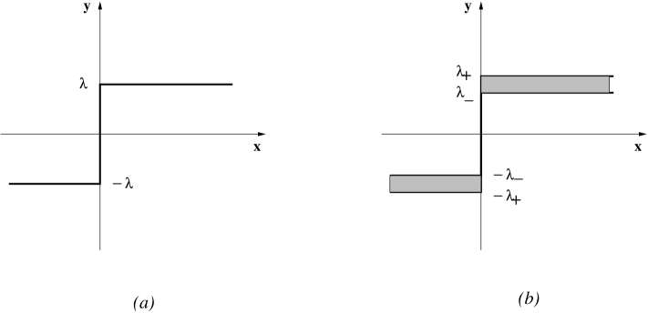
Figure 5.1: Plasticity law. (a): ideal law with thin line. (b): law with thick line

In figure 5.1, a pictural representation of the blurred law is a graph with ”thick line” (displayed at the right) in contrast to the ideal law with a ”thin line” (displayed at the left).

Proposition 5.1

The blurred plastic law with the graph $M$ (5.0.2) is represented by the bipotential:

$$b(x,y)=sup\left(\lambda_{-},\parallel y\parallel\right)\parallel x\parallel+\chi_{B(\lambda_{+})}(y)$$ (5.0.3)

with the notation $\lambda_{\pm}=\lambda\pm\epsilon$.

Equivalently, the relation $y\in\partial\phi(x)+a$, $\|a\|\leq\varepsilon$, can be put in the form $y\in\partial b(\cdot,y)(x)$, with $b$ the bipotential defined by (5.0.3).

Proof.

As previously, we intend to construct a bipotential for $M$ from a bipotential convex cover. This time $a$ is not the good parameter for a bipotential convex cover because it is difficult to check all the conditions of Theorem 3.3 for this parameter.

The bipotential convex cover will have as parameter a variable yielding threshold $\eta$ taking arbitrary values in $[\lambda_{-},\lambda_{+}]$ where $\lambda_{\pm}=\lambda\pm\epsilon$. The graph $M$ (5.0.2 ) admits the description:

$$M=\left\{(0,y)\in X\times Y\ \mid\ \parallel y\parallel<\lambda_{-}\right\}\cup$$ (5.0.4)

$$\cup\left\{(x,y)\in X\times Y\ \mid\ \lambda_{-}\leq\parallel y\parallel\leq\lambda_{+}\ and\ \exists\eta\geq 0,\ x=\eta y\right\}$$

Let $\left\{b_{\eta}\mbox{ : }\eta\in[\lambda_{-},\lambda_{+}]\right\}$ be the collection of separated bipotentials:

$$f(\eta,x,y)=b_{\eta}(x,y)\ =\ \eta\|x\|+\chi_{B(\eta)}(y)\ .$$

We shall verify that this is a bipotential convex cover of $M$. Indeed, the conditions (a) to (c) of Definition 3.2 are obviously fulfilled. With $f(\eta,x,y)=b_{\eta}(x,y)$, we have to prove the last condition (d). For the implicit convexity of $f(\cdot,\cdot,y)$ we have to prove that for any $x_{1},x_{2}\in X$, $y\in Y$, $\eta_{1},\eta_{2}\in[\lambda_{-},\lambda_{+}]$, $\alpha,\beta\in[0,1]$, $\alpha+\beta=1$ there exists $\eta\in[\lambda_{-},\lambda_{+}]$ such that:

$$\alpha\eta_{1}\parallel x_{1}\parallel+\beta\eta_{2}\parallel x_{2}\parallel+\chi_{B(\eta_{1})}(y)+\chi_{B(\eta_{2})}(y)\geq\eta\parallel\alpha x_{1}+\beta x_{2}\parallel+\chi_{B(\eta)}(y)\ .$$

We choose $\eta=\min(\eta_{1},\eta_{2})$. The previous inequality becomes: for any $\parallel y\parallel\leq\eta$

$$\alpha\eta_{1}\parallel x_{1}\parallel+\beta\eta_{2}\parallel x_{2}\parallel\geq\eta\parallel\alpha x_{1}+\beta x_{2}\parallel\ ,$$

which is true because of the convexity of the norm.

For the implicit convexity of $f(\cdot,x,\cdot)$ we have to prove that: for any $x\in X$, $y_{1},y_{2}\in Y$, $\eta_{1},\eta_{2}\in[\lambda_{-},\lambda_{+}]$, $\alpha,\beta\in[0,1]$, $\alpha+\beta=1$there exists $\eta\in[\lambda_{-},\lambda_{+}]$ such that:

$$(\alpha\eta_{1}+\beta\eta_{2})\ \parallel x\parallel+\chi_{B(\eta_{1})}(y_{1})+\chi_{B(\eta_{2})}(y_{2})\geq\eta\parallel x\parallel+\chi_{B(\eta)}(\alpha y_{1}+\beta y_{2})$$

This time we choose $\eta=\alpha\eta_{1}+\beta\eta_{2}$. Indeed, for any $\parallel y_{1}\parallel\leq\lambda_{1}$ and $\parallel y_{2}\parallel\leq\lambda_{2}$, we have:

$$\parallel\alpha y_{1}+\beta y_{2}\parallel\ \leq\ \alpha\parallel y_{1}\parallel+\beta\parallel y_{2}\parallel\ \leq\ \alpha\eta_{1}+\beta\eta_{2}=\eta$$

therefore the inequality we want to prove becomes trivial:

$$(\alpha\eta_{1}+\beta\eta_{2})\ \parallel x\parallel\geq\eta\parallel x\parallel\ .$$

Hence we are in the conditions of applying Theorem 3.3. The graph $M$ admits the bipotential

$$b(x,y)\ =\ \inf\left\{\lambda\|x\|+\chi_{B(\lambda)}(y)\mbox{ : }\lambda\in[\lambda_{-},\lambda_{+}]\right\}\ .$$

In order to compute $b$, three events have to be considered:

1. for $\parallel y\parallel>\lambda_{+}$, $b(x,y)\ =+\infty\$ ,

2. for $\lambda_{-}\leq\parallel y\parallel\leq\lambda_{+}$, $b(x,y)\ =\ \inf\left\{\lambda\|x\|\mbox{ : }\parallel y\parallel<\lambda\leq\lambda_{+}\right\}\ =\ \|y\|\|x\|\$,

3. for $\parallel y\parallel\leq\lambda_{-}$, $b(x,y)\ =\ \inf\left\{\lambda\|x\|\mbox{ : }\lambda_{-}\leq\lambda\leq\lambda_{+}\right\}\ =\ \lambda_{-}\|x\|\$.

The proof is done.  $\square$

6 Application to a blurred Coulomb’s friction law

The law of unilateral contact with Coulomb’s dry friction is a typical example of what is called a non associated constitutive law in mechanics. Despite of its rather complex structure, it is worthwhile to have interest in it because of its importance in many practical problems.

We shall not discuss here the phenomenal and experimental aspects but only the mathematical modeling with respect to the bipotential theory. To be short, the space $X=\mathbb{R}^{3}$ is the one of relative velocities between points of two bodies, and the space $Y$, identified also to $\mathbb{R}^{3}$, is the one of the contact reaction stresses. The duality product is the usual scalar product. We put

$$(x_{n},x_{t})\in X=\mathbb{R}\times\mathbb{R}^{2},\quad(y_{n},y_{t})\in Y=\mathbb{R}\times\mathbb{R}^{2}\ ,$$

where $x_{n}$ is the gap velocity, $x_{t}$ is the sliding velocity, $y_{n}$ is the contact pressure and $y_{t}$ is minus the friction stress. The friction coefficient is $\mu>0$. The graph of the law of unilateral contact with Coulomb’s dry friction is defined as the union of three sets, respectively corresponding to the ’body separation’, the ’sticking’ and the ’sliding’.

$$M_{\mu}=\left\{(x,0)\in X\times Y\ \mid\ x_{n}<0\right\}\cup\left\{(0,y)\in X\times Y\ \mid\ \parallel y_{t}\parallel\leq\mu y_{n}\right\}\cup$$ (6.0.1)

$$\cup\left\{(x,y)\in X\times Y\ \mid\ x_{n}=0,\ x_{t}\neq 0,\ y_{t}=\mu y_{n}\dfrac{x_{t}}{\parallel x_{t}\parallel}\right\}$$

It is well known that this graph is not monotone, then not cyclically monotone. As usual, we introduce Coulomb’s cone

$$K_{\mu}=\left\{(y_{n},y_{t})\in Y\ \mid\ \parallel y_{t}\parallel\leq\mu y_{n}\right\},$$

and its conjugate cone

$$K_{\mu}^{*}=\left\{(x_{n},x_{t})\in X\ \mid\ \mu\parallel x_{t}\parallel+x_{n}\leq 0\right\}.$$

In particular, we have

$$K_{0}=\left\{(y_{n},0)\in Y\ \mid\ y_{n}\geq 0\right\},\quad K_{0}^{*}=\left\{(x_{n},x_{t})\in X\ \mid\ x_{n}\leq 0\right\}.$$

In [5], [6], we obtained as application of Theorem 3.3 the following expression:

$$b_{\mu}(x,y)\ =\mu y_{n}\parallel x_{t}\parallel+\chi_{K_{\mu}}(y)+\chi_{K^{*}_{0}}(x)$$ (6.0.2)

recovering the bipotential firstly obtained in heuristic way in [13].

We shall modify the unilateral contact law with Coulomb’s dry friction by allowing arbitrary values for the friction coefficient $\mu$ in a range $\left[\mu_{-},\mu_{+}\right]$, that leads to the blurred friction law represented by the graph:

$$M=\left\{(x,0)\in X\times Y\ \mid\ x_{n}<0\right\}\cup$$ (6.0.3)

$$\cup\left\{(0,y)\in X\times Y\ \mid\ \mu_{-}y_{n}\leq\parallel y_{t}\parallel\leq\mu_{+}y_{n},\ \ \exists\eta\geq 0,\ \ x_{t}=\eta y_{t}\right\}$$

Proposition 6.1

The blurred plastic law with the graph $M$ (6.0.3) is represented by the bipotential:

$$b(x,y)=\sup\left(\mu_{-}y_{n},\parallel y_{t}\parallel\right)\parallel x_{t}\parallel+\chi_{K_{\mu_{+}}}(y)+\ \chi_{K^{*}_{0}}(x)$$ (6.0.4)

Equivalently, the relation $y\in\partial b_{\mu}(\cdot,y)$, $\mu\in\left[\mu_{-},\mu_{+}\right]$, with $b_{\mu}$ defined by (6.0.2), can be put in the form $y\in\partial b(\cdot,y)(x)$, with $b$ the bipotential defined by (6.0.4).

Proof.

The collection $\left\{b_{\mu}\mbox{ : }\mu\in[\mu_{-},\mu_{+}]\right\}$ of bipotentials $b_{\mu}$ defined as in (6.0.2) is a bipotential convex cover. The demonstration of the conditions of Definition 3.2 is similar to the one of the blurred plasticity law and is not reproduced here.

Applying Theorem 3.3, the graph (6.0.3) of the blurred law admits the bipotential:

$$b(x,y)\ =\ \inf\left\{\mu y_{n}\parallel x_{t}\parallel+\chi_{K_{\mu}}(y)\mbox{ : }\mu\in[\mu_{-},\mu_{+}]\right\}\ +\ \chi_{K^{*}_{0}}(x)\ .$$

We shall compute this bipotential. If $x\in K^{*}_{0}$ , three events have to be considered:

1. for $\parallel y_{t}\parallel>\mu_{+}y_{n}$, $b(x,y)\ =+\infty\$ ,

2. for $\mu_{-}y_{n}\leq\parallel y_{t}\parallel\leq\mu_{+}y_{n}$, $b(x,y)\ =\ \inf\left\{\mu y_{n}\|x_{t}\|\mbox{ : }\parallel y_{t}\parallel<\mu y_{n}\leq\mu_{+}y_{n}\right\}\ =\ \|y_{t}\|\|x_{t}\|\$,

3. for $\parallel y_{t}\parallel\leq\mu_{-}y_{n}$, $b(x,y)\ =\ \inf\left\{\mu y_{n}\|x_{t}\|\mbox{ : }\mu_{-}\leq\mu\leq\mu_{+}\right\}\ =\ \mu_{-}y_{n}\|x_{t}\|\$.

If $x$ does not belongs to $K^{*}_{0}$ , $b(x,y)\ =+\infty\$. In short, the blurred Coulomb friction contact law given by the graph 6.0.3 admits the bipotential (6.0.4).  $\square$

7 Conclusion

We showed how the bipotential method is able to capture blurred constitutive laws. The blurring of a constitutive law enters by allowing some error in the law with a fixed margin of tolerance. For example a material parameter takes indeterminate values in a compact set modeling some experimental incertitudes. The notion of bipotential convex cover leads to the construction of a bipotential for such a blurred constitutive law. These bipotentials could be used to represent structural mechanics problems with blurred constitutive laws by means of variational inequalities.

References

- [1] G. Bodovillé: On damage and implicit standard materials, C. R. Acad. Sci., Paris, Sér. II, Fasc. b, Méc. Phys. Astron. 327(8) (1999) 715-720.
- [2] G. Bodovillé, G. de Saxcé: Plasticity with non linear kinematic hardening : modelling and shakedown analysis by the bipotential approach, Eur. J. Mech., A/Solids, 20 (2001) 99-112.
- [3] L. Bousshine, A. Chaaba, G. de Saxcé: Plastic limit load of plane frames with frictional contact supports, Int. J. Mech. Sci. 44(11) (2002) 2189-2216.
- [4] M. Buliga, G. de Saxcé, C. Vallée: Existence and construction of bipotentials for graphs of multivalued laws, J. Convex Analysis 15(1) (2008) 87-104.
- [5] M. Buliga, G. de Saxcé, C. Vallée: Bipotentials for non monotone multivalued operators: fundamental results and applications, Acta Applicandae Mathematicae (2009), DOI 10.1007/s10440-009-9488-3.
- [6] M. Buliga, G. de Saxcé, C. Vallée: Non maximal cyclically monotone graphs and construction of a bipotential for the Coulomb’s dry friction law, J. Convex Analysis 17(1) (2010).
- [7] Z.-Q. Feng, M. Hjiaj, G. de Saxcé, Z. Mróz: Effect of frictional anisotropy on the quasistatic motion of a deformable solid sliding on a planar surface, Comput. Mech. 37 (2006) 349-361.
- [8] J. Fortin, M. Hjiaj, G. de Saxcé: An improved discrete element method based on a variational formulation of the frictional contact law, Comput. Geotech. 29(8) (2002) 609-640.
- [9] B. Halphen, Nguyen Quoc Son: Sur les matériaux standard généralisés, J. Méc., Paris 14 (1975) 39-63.
- [10] M. Hjiaj, G. Bodovillé, G. de Saxcé: Matériaux viscoplastiques et loi de normalité implicites, C. R. Acad. Sci., Paris, Sér. II, Fasc. b, Méc. Phys. Astron. 328 (2000) 519-524.
- [11] M. Hjiaj, Z.-Q. Feng, G. de Saxcé, Z. Mróz: Three dimensional finite element computations for frictional contact problems with on-associated sliding rule, Int. J. Numer. Methods Eng. 60(12) (2004) 2045-2076.
- [12] P. Laborde, Y. Renard: Fixed points strategies for elastostatic frictional contact problems. Math. Meth. Appl. Sci. 31 (2008) 415-441.
- [13] G. de Saxcé, Z.Q. Feng: New inequation and functional for contact with friction: the implicit standard material approach, Mech. Struct. and Mach. 19(3) (1991) 301-325.
- [14] G. de Saxcé: Une généralisation de l’inégalité de Fenchel et ses applications aux lois constitutives, C. R. Acad. Sci., Paris, Sér. II 314 (1992) 125-129.
- [15] G. de Saxcé, L. Bousshine: On the extension of limit analysis theorems to the non associated flow rules in soils and to the contact with Coulomb’s friction, in: Proc. XI Polish Conference on Computer Methods in Mechanics (Kielce, 1993), Vol. 2 (1993) 815-822.
- [16] G. de Saxcé: The bipotential method, a new variational and numerical treatment of the dissipative laws of materials, in: Proc. 10th Int. Conf. on Mathematical and Computer Modelling and Scientific Computing, (Boston, 1995).
- [17] G. de Saxcé, L. Bousshine: Implicit standard materials, in: Inelastic behaviour of structures under variable repeated loads, D. Weichert G. Maier (eds.), CISM Courses and Lectures 432, Springer, Wien (2002).
- [18] G. de Saxcé, Z.-Q. Feng: The bipotential method: a constructive approach to design the complete contact law with friction and improved numerical algorithms, Math. Comput. 28(4-8) (1998) 225-245.
- [19] C. Vallée, C. Lerintiu, D. Fortuné, M. Ban, G. de Saxcé: Hill’s bipotential, in: New Trends in Continuum Mechanics, M. Mihailescu-Suliciu (ed.), Theta Series in Advanced Mathematics, Theta Foundation, Bucarest (2005) 339-351.
- [20] I. Babuska, W.C. Rheinboldt: A posteriori estimates for the finite element method, Int. J. Numer. Methods Engrg. 12 (1978) 1597-1615.
- [21] I. Babuska, W.C. Rheinboldt: Adaptive approaches and reliability estimators in finite element analysis, Comput. Methods Applied Mech. Engrg. 17/18 (1979) 519-540.
- [22] D.W. Kelly, J. Gago, O.C. Zienkiewicz, I. Babuska, A posteriori error analysis and adaptative processes in finite element method. Part 1: Error analysis, Int. J. Numer. Methods Engrg. 19 (1983) 1593-1619.
- [23] J. Gago, D.W. Kelly, O.C. Zienkiewicz, I. Babuska, A posteriori error analysis and adaptative processes in finite element method. Part 2: Adaptative mesh refinement, Int. J. Numer. Methods Engrg. 19 (1983) 1921-1656.
- [24] J.T. Oden, L. Demkowicz, W. Rachowicz, T.A. Westermann, Toward a universal h-p adaptative finite element strategy, Part 2: A posteriori error estimation, Comput. Methods Appl. Mech. Engrg. 77 (1989) 113-180.
- [25] O.C. Zienkiewicz, J.Z. Zhu, A simple error estimator and adaptative procedure for practical engineering analysis, Int. J. Numer. Methods Engrg. 24 (1987) 337-357.
- [26] O.C. Zienkiewicz, J.Z. Zhu, The superconvergent patch recovery and a posteriori error estimates, Part 1: The recovery technique, Int. J. Numer. Methods Engrg. 33 (1992) 1331-1364.
- [27] O.C. Zienkiewicz, J.Z. Zhu, The superconvergent patch recovery and a posteriori error estimates, Part 2: Error estimates and adaptativity, Int. J. Numer. Methods Engrg. 33 (1992) 1365-1382.
- [28] B. Fraeijs de Veubeke, Displacement and equilibrium models in the finite element method, in: O.C. Zienkiewicz, ed., Stress Analysis Chap. 9 (John Wiley, 1965).
- [29] J.F. Debongnie, H.G. Zhong, P. Beckers, Dual analysis with general boundary conditions, Comput. Methods. Appl. Mech. Engrg. 122 (1995) 183-192.
- [30] P. Ladevèze, Comparaisons de modèles de milieux continus, Thèse d’Etat, Université Pierre et Marie Curie, Paris (1975).
- [31] P. Ladevèze, G. Coffignal, J.P. Pelle, Accuracy of elastoplastic and dynamic analysis, in: I. Babuska, J. Gago, E. Oliveira and O.C. Zienkiewicz, eds., Accuracy Estimates and Adaptative Refinements in Finite Element Computations (John Wiley, 1986) 181-203.
- [32] P. Ladevèze, J.P. Pelle, P. Rougeot, Error estimation and mesh optimization for classical finite element, Engrg. Comput. 8 (1991) 69-80.
- [33] P. Ladevèze, La maîtrise des modèles en mécanique des structures, Revue européenne des éléments finis 1 (1992) 9-30.
- [34] P. Ladevèze, N. Moes, A new a posteriori error estimation for nonlinear time-dependent finite element analysis, Comput. Methods. Appl. Mech. Engrg. 157 (1997) 45-68.
- [35] P. Ladevèze, J.P. Pelle, La maîtrise du calcul en mécanique linéaire et non linéaire, (Hermes Science, 2001).
- [36] Pierre Ladevèze, E. Florentin, Verification of stochastic models in uncertain environments using the constitutive relation error method, Comput. Methods. Appl. Mech. Engrg. 196 (2006) 225-224.
- [37] P. Ladevèze, G. Puel, A. Deraemaeker, T. Romeuf, Validation of structural dynamics models containing uncertainties, Comput. Methods. Appl. Mech. Engrg. 195 (2006) 373-393.