Estimating eddy diffusivities from noisy Lagrangian observations

Abstract

The problem of estimating the eddy diffusivity from Lagrangian observations in the presence of measurement error is studied in this paper. We consider a class of incompressible velocity fields for which is can be rigorously proved that the small scale dynamics can be parameterised in terms of an eddy diffusivity tensor. We show, by means of analysis and numerical experiments, that subsampling of the data is necessary for the accurate estimation of the eddy diffusivity. The optimal sampling rate depends on the detailed properties of the velocity field. Furthermore, we show that averaging over the data only marginally reduces the bias of the estimator due to the multiscale structure of the problem, but that it does significantly reduce the effect of observation error.

1 Introduction

Many phenomena in the physical sciences involve a multitude of characteristic temporal and spatial scales. In most cases it is not only impossible to study the behavior of the phenomenon at all scales, but it is also unnecessary, since usually one is interested in the evolution of a few variables which describe the dynamics at large scales. It is, therefore, important to develop systematic methods for deriving simplified coarse grained models that capture the essential features of the systems at long scales, while accurately parameterising the small scales. In recent years it has become clear that the use of data, together with coarse graining procedures, is essential for the accurate parameterisation of small scales [GKS04, CVE06a, CVE06b, HKDS07, HS08]. The aim of this paper is to study problems of this form in the context of transport of passive tracers.

We are particularly motivated by the challenge of using Lagrangian float data to inform the design of subgrid mixing schemes for advected tracers in ocean models. The vast amount of Lagrangian float data available (for example, the ARGO project has 3000 floats in current operation [ARGO06]) presents the opportunity to develop data-driven model reduction techniques. Lagrangian data are particularly suitable for statistical studies of the transport of passively advected substances in the ocean, with the simplest statistical description of transport phenomena provided by the average concentration of a passive tracer.

In this paper, we assume that the Lagrangian trajectories are given by the following stochastic differential equation:

$$\dot{x}=v(x,t)+\sqrt{2\kappa}\dot{W}.$$ (1.1)

Here $x(t)\in\mathbb{R}^{d}$ represents the Lagrangian path, $v(x,t)$ is a (prescribed) incompressible velocity field, $\kappa$ is the small-scale diffusivity and $W(t)$ denotes standard Brownian motion in $\mathbb{R}^{d}$. More sophisticated models have been proposed for oceanographic applications, for example [BM02, BM03, Pit02, Wig05, GOPR95].

We wish to extract the coarse grained (large length scale and long time scale) dynamics of solutions of equation (1.1). For a wide class of velocity fields (deterministic space-time periodic, Gaussian random fields etc.), it is well known [MK99, PS08, BLP78] that, at sufficiently long length and time scales, the dynamics of (1.1) becomes Brownian and can be described by the eddy diffusivity tensor. More precisely, it is possible to prove that solutions of (1.1) converge, under the diffusive rescaling and assuming that the velocity field has zero mean, to an effective Brownian motion

$$\lim_{\epsilon\rightarrow 0}\epsilon x(t/\epsilon^{2})=\sqrt{2\mathcal{K}}W(t),$$ (1.2)

weakly on $C([0,T];\mathbb{R}^{d})$, where $W(t)$ is a standard Brownian motion on $\mathbb{R}^{d}$ and $\mathcal{K}$ denotes the eddy (effective) diffusivity tensor. The tensor $\mathcal{K}$ represents the effective diffusivity caused by the interaction of molecular diffusion with the transport properties of $v$.

Consequently, at large length scales and long time scales the dynamics of the passive tracer is governed by an equation of the form

$$\dot{X}=\sqrt{2\mathcal{K}}\dot{W}.$$ (1.3)

It is quite often the case (in designing subgrid mixing schemes for example) that we only wish to calculate the eddy diffusivity, rather than the detailed properties of the velocity field $v(x,t)$ at all scales. It is then necessary to estimate the eddy diffusivity of a passive tracer from Lagrangian observations. In this paper we address precisely this issue: given a Lagrangian trajectory which is consistent with (1.1) in the presence of observation noise, how can we estimate the eddy diffusivity $\mathcal{K}$? This problem has been studied quite extensively over the last few years [BSG02, FO94, Fig94, BSGMO98, VGRM04].

More generally, we might also want to estimate other coarse grained quantities such as the effective drift, or we might want to consider a space dependent eddy diffusivity. This is a challenging problem in statistical inference: data sampled from (1.1) is only consistent with (1.3) at sufficiently large scales. In other words, the difficulty stems from the fact that the model (1.3) used for fitting the data is the wrong model, apart from the large scale part of the data. Furthermore, we do not know a priori the length and time scales on which the coarse grained model (1.3) is valid. On the other hand, we can perform statistical inference in a fully parametric setting for (1.3), since only the eddy diffusivity needs to be estimated; statistical inference for (1.1) would require the non-parametric estimation of the velocity field $v(x,t)$ [CDRS09]. Parameter estimation for diffusion processes under misspecified or incorrect models has been studied in the statistics literature [Kut04, Sec 2.6.1].

The problem of parameter estimation for a model that is incompatible with the available data at small scales was studied in [PS07, PPS08a, PPS08b] for a class of fast-slow systems of SDEs for which the existence of a coarse grained equation for the slow variables can be proved rigorously. In these papers, parameter estimation for the averaging problem

$$\frac{dx}{dt} = f_{1}(x,y)+\alpha_{0}(x,y)\frac{dU}{dt}+\alpha_{1}(x,y)\frac{dV}{dt},$$ (1.4a)

$$\frac{dy}{dt} = \frac{1}{\epsilon}g_{0}(x,y)+\frac{1}{\sqrt{\epsilon}}\beta(x,y)\frac{dV}{dt};$$ (1.4b)

as well as for the homogenization problem

$$\frac{dx}{dt} = \frac{1}{\epsilon}f_{0}(x,y)+f_{1}(x,y)+\alpha_{0}(x,y)\frac{dU}{dt}+\alpha_{1}(x,y)\frac{dV}{dt},$$ (1.5a)

$$\frac{dy}{dt} = \frac{1}{\epsilon^{2}}g_{0}(x,y)+\frac{1}{\epsilon}g_{1}(x,y)+\frac{1}{\epsilon}\beta(x,y)\frac{dV}{dt}.$$ (1.5b)

was studied. In both cases the goal was to fit data obtained from (1.4a) or (1.5a) to the coarse grained equation

$$\frac{dX}{dt}=F(X;\theta)+K(X)\frac{dW}{dt},$$ (1.6)

which describes the dynamics of the slow variable $x(t)$ in the limit as $\epsilon\rightarrow 0$. In the aforementioned papers, it was assumed that the vector field $F(X;\theta)$ depends on a set of parameters $\theta$ that we want to estimate using data taken from either the averaging or the homogenization problem. For the homogenization problem it was shown in [PPS08a] that the maximum likelihood estimator is asymptotically biased. In particular, it is necessary to subsample at an appropriate rate in order to estimate the parameters $\theta$ accurately. Similar issues were investigated for the thermal motion of a particle in a multiscale potential [PS07]. It was shown that subsampling is necessary for the accurate estimation of the drift and diffusion coefficients.

Related issues have been studied in the field of econometrics. In this context, the question is how to accurately estimate the integrated stochastic volatility when market microstructure noise (i.e. additive white noise) is present. It was shown in [ASMZ05b, ASMZ05a] that subsampling reduces the bias in the estimator. It was also shown that subsampling combined with averaging and an appropriate de-biasing step can lead to an accurate and efficient estimator for the integrated stochastic volatility.

In this paper we will study the problem of estimating the eddy diffusivity from noisy Lagrangian observations:

$$y_{t_{j}}=x_{t_{j}}+\theta\epsilon_{t_{j}},\quad j=1,\dots N,$$

where $\{x_{0},x_{1},\ldots,x_{N}\}$ is a set of samples from a trajectory consistent with equation (1.1), $\epsilon_{t_{j}}$ are independent $\mathcal{N}(0,1)$ random variables modelling the observation error, and $\theta$ measures the strength of the observation error.

We will consider time-independent spatially-periodic incompressible velocity fields as well as spatially-periodic velocity fields that are modulated in time by a time-periodic function, or a Gaussian process. In all of these cases, the rescaled trajectory converges weakly to a Brownian motion (1.2) (see [PS08, Ch. 13]). The eddy diffusivity depends in a highly nonlinear way on the properties of the velocity field $v(x,t)$. It can be shown (for the class of velocity fields considered in this paper) that the eddy diffusivity $\mathcal{K}$ satisfies the upper and lower bounds (we use the notation $\mathcal{K}^{\xi}=\langle\xi,\mathcal{K}\xi\rangle$ where $\xi$ is an arbitrary vector in $\mathbb{R}^{d}$) [AM91]

$$\kappa\leq\mathcal{K}^{\xi}\leq\frac{C}{\kappa},$$ (1.7)

for $\kappa$ sufficiently small and some positive constant $C$. We will consider the physically interesting regime $\kappa\ll 1$.

As an eddy diffusivity estimator we will use the quadratic variation

$$\mathcal{K}_{N,\delta}=\frac{1}{2N\delta}\sum_{n=0}^{N-1}\big{(}x_{n+1}-x_{n}\big{)}\otimes\big{(}x_{n+1}-x_{n}\big{)},$$ (1.8)

where $N$ is the number of observations which we assume to be equidistant, with the distance between two subsequent observations being $\delta$, and $T=N\delta$. It is well known [BR80] that, for an SDE of the form (1.1), we have the convergence result

$$\lim_{N\rightarrow\infty}\sum_{j=0}^{N-1}\big{(}x_{(j+1)T2^{-N}}-x_{jT2^{-N}}\big{)}\otimes\big{(}x_{(j+1)T2^{-N}}-x_{jT2^{-N}}\big{)}=2\kappa IT,\quad\mbox{a.s.}$$ (1.9)

where $I$ denotes the unit matrix. If we write equation (1.9) with $x_{i}$ replaced by $y_{i}$, the quadratic variation diverges in the limit as $N\to\infty$ due to the observation error. In view of the bounds (1.7), it becomes clear that that the estimator $\mathcal{K}_{N,\delta}$ underestimates the value of the eddy diffusivity in this limit. In particular, when the eddy diffusivity scales like $\kappa^{-1}$ the estimator (1.8) can underestimate the eddy diffusivity by several orders of magnitude.

The above suggests that in order to be able to estimate the eddy diffusivity from Lagrangian data, subsampling at an appropriate rate is necessary. However, it is not clear a priori what the sampling rate should be. Roughly speaking, we need to look at the data at the scale for which the coarse grained description (1.3) is valid. The estimation of this time scale is a difficult dynamical question that has been addressed only partially  [Fan02, HP08]. The diffusive time, the time that it takes for the Lagrangian particle to reach the asymptotic regime described by a Brownian motion with diffusion matrix $\mathcal{K}$ depends crucially on the streamline topology and is related to the scaling of the eddy diffusivity with $\kappa$. Clearly we have two sources of error: measurement error, and the error in the estimation of parameters from reduced models using data from the full dynamics which we refer to as the multiscale error. The multiscale error is precisely due to the fact that the reduced model is incompatible with the data at small scales.

In this paper we study the small $\kappa$ asymptotics of the quadratic variation (1.8). We show, by means of rigorous analysis and numerical experiments, that, unless we subsample at an appropriate rate, we cannot estimate the eddy diffusivity from the quadratic variation, due to the multiscale error. Additionally, we show that for smooth time-independent spatially periodic velocity fields, the scaling of the optimal sampling rate with $\kappa$ depends on the detailed properties of the velocity field. Our analysis is based on standard limit theorems for stochastic processes, together with careful study of a Poisson equation posed on the unit torus.

From the point of view of statistics, it is clearly not optimal to simply ignore most of the available data by subsampling. It is natural, therefore, to try to use all data through averaging. We experiment with two different types of averaging: box averaging (computing the quadratic variation using local averages), and shift averaging (which is related to the moving averaging method of statistics). We show by means of numerical experiments, that shift averaging significantly reduces the effects of observation error, but only marginally reduces the multiscale error. On the other hand, box averaging increases the bias of the estimator.

We emphasize that the setting in which we are working is related to but different from the problems studied in [PS07, PPS08a, PPS08b]. In particular, we do not assume a priori that we have scale separation and that we know the value of the parameter $\epsilon$ which measures the degree of scale separation. Rather, the scale separation is induced by the dynamics of (1.1). The time scale at which the coarse grained description is valid is essentially what we need to estimate, since this provides us with information about the appropriate sampling rate. For completeness, we also consider the rescaled problem (2.10) below. The rescaled problem and the original one are equivalent under space-time rescaling for time-independent velocity fields. However, from the point of view of estimating the eddy diffusivity they lead to different problems. When using the quadratic variation to estimate the eddy diffusivity in equation (1.1) we actually study the small $\kappa$ limit, whereas for the rescaled problem we study the limit of infinite scale separation while keeping $\kappa$ fixed.

The rest of the paper is organized as follows. In Section 2 we we study the problem of estimating the eddy diffusivity using Lagrangian observations from the rescaled equation. In Section 3 we study the same problem for the unscaled equation (1.1), and we also study the effect of observation error on the estimator. In Section 4 we develop estimators for the eddy diffusivity which are based on a combination of subsampling with averaging and present numerical results for various types of two-dimensional velocity fields. Summary and conclusions are presented in Section 5. Some technical results are included in the appendices.

2 The Rescaled Problem

We consider the equation for the rescaled process

$$x^{\epsilon}(t)=\epsilon x(t/\epsilon^{2}),$$

given by

$$\frac{dx}{dt}=\frac{1}{\epsilon}v\left(\frac{x}{\epsilon}\right)+\sqrt{2\kappa}\dot{W},$$ (2.10)

where we have dropped the superscript $\epsilon$ for notational simplicity.. Our goal is to estimate the eddy diffusivity using data from (2.10), in the parameter regime $\epsilon\ll 1$ and for $\kappa$ fixed. In particular, we want to find how the sampling rate should scale with $\epsilon$ for the accurate estimation of the eddy diffusivity using the quadratic variation estimator. The main result of this section is that, provided that the sampling rate is in between the two characteristic time scales $1$ and $\epsilon$ of the problem, then the estimator (1.8) is asymptotically unbiased, in the limit as $\epsilon\to 0.$

We assume that the velocity field is smooth, divergence-free, mean zero and $1-$periodic, i.e. periodic with period $1$ in each Cartesian direction. Under these assumptions, the solution to (2.10) converges weakly on $C([0,T];\mathbb{R}^{d})$ to $X$, as $\epsilon\rightarrow 0$, the solution of

$$\frac{dX}{dt}=\sqrt{2\mathcal{K}}\frac{dW}{dt},$$

as $\epsilon\to 0$. The eddy diffusivity is given by the formula

$$\mathcal{K}=\kappa I+\kappa\int_{\mathbb{T}^{d}}\nabla_{z}\chi(z)\otimes\nabla_{z}\chi(z)\,dz$$ (2.11)

where the vector field $\chi(z)$ is the solution of the PDE

$$-\mathcal{L}_{0}\chi(z)=v(z)$$ (2.12)

on $\mathbb{T}^{d}$ with periodic boundary conditions, and where $\mathcal{L}_{0}$ is the generator of the Markov process $z$ on $\mathbb{T}^{d}$:

$$\frac{dz}{dt}=v(z)+\sqrt{2\kappa}\frac{dW}{dt},$$ (2.13)

i.e.

$$\mathcal{L}_{0}=v(z)\cdot\nabla_{z}+\kappa\Delta_{z},$$

with periodic boundary conditions. We refer to [PS08] for the derivation of this result.

Now let $\mathcal{K}^{\xi}=\xi\cdot\mathcal{K}\xi$ where $\xi\in\mathbb{R}^{d}$ arbitrary. From (2.11) it easily follows that

$$\mathcal{K}^{\xi}=\kappa\int_{\mathbb{T}^{d}}|\xi+\nabla_{z}\chi^{\xi}|^{2}\,dz,$$ (2.14)

where $\chi^{\xi}=\chi\cdot\xi$. Let $\mathcal{K}^{\xi}_{N,\delta}$ be the quadratic variation along the direction $\xi$:

$$\mathcal{K}^{\xi}_{N,\delta}=\frac{1}{2N\delta}\sum_{n=0}^{N-1}\big{(}x_{n+1}^{\xi}-x^{\xi}_{n}\big{)}^{2},$$ (2.15)

where $x^{\xi}_{n}=x(n\delta)\cdot\xi$.

Our goal is to find how the sampling rate $\delta$ should be chosen so that we can estimate the component of the eddy diffusivity (2.11) along the direction $\xi$ using (2.15). The following theorem states that the estimator converges in $L^{2}$ to the eddy diffusivity in the limit $\epsilon\to 0$, $N\to\infty$, with $T$ fixed.

Theorem 2.1.

Let $v(z)$ be a smooth, divergence-free, mean zero, 1-periodic vector field and assume that the process $z$ defined in (2.13) is stationary. Then

$$\mathbb{E}|\mathcal{K}_{N,\delta}^{\xi}-\mathcal{K}^{\xi}|^{2}\leq\frac{C}{N}+C\big{(}\epsilon^{4}\delta^{-2}+\epsilon^{3}\delta^{-3/2}+\epsilon^{2}\delta^{-1}+\epsilon\delta^{-1/2}\big{)}.$$ (2.16)

In particular, when $\delta=\epsilon^{\alpha},\,\alpha\in(0,2)$, we have

$$\lim_{N\rightarrow+\infty}\lim_{\epsilon\rightarrow 0}\mathbb{E}|\mathcal{K}^{\xi}_{N,\delta}-\mathcal{K}^{\xi}|^{2}=0,$$

for $N\delta=T$ fixed (i.e. $N\sim\epsilon^{-\alpha}$).

Remark 2.2.

The scaling of the optimal sampling rate with $\epsilon$, $\delta\sim\epsilon^{\alpha},$ with $\alpha\in(0,2)$ appears to be sharp and it is expected on intuitive grounds, since one would expect that the optimal sampling rate should be in between the two characteristic time scales of the problem $1$ and $\epsilon^{2}$.

Remark 2.3.

The stationarity assumption on $z$ can be removed since even when $z$ starts with arbitrary initial conditions its law converges exponentially fast to the invariant measure of the process which is the Lebesgue measure on $\mathbb{T}^{d}$. We refer to [Bat99] for the details.

For the proof of this theorem we will need the following lemma.

Lemma 2.4.

Let $v(z)$ be a smooth, divergence-free, mean zero, 1-periodic vector field and assume that the process $z$ defined in (2.13) is stationary. Then

$$|\mathbb{E}\mathcal{K}^{\xi}_{N,\delta}-\mathcal{K}^{\xi}|\leq C\big{(}\epsilon^{2}\delta^{-1}+\epsilon\delta^{-1/2}\big{)}.$$

In particular, when $\delta=\epsilon^{\alpha},\,\alpha\in(0,2)$ we have

$$\lim_{\epsilon\rightarrow 0}|\mathbb{E}\mathcal{K}^{\xi}_{N,\delta}-\mathcal{K}^{\xi}|=0.$$

Remark 2.5.

Notice that in order for the expectation of the quadratic variation to converge to the eddy diffusivity it is not necessary to take the limit $N\rightarrow\infty$. Of course, in order to keep $N\delta=T$ fixed we need to take $N\sim\delta^{-1}=\kappa^{-\alpha}$.

Proof of Lemma 2.4 With the help of the auxiliary process $z=x/\epsilon\in\mathbb{T}^{d}$, equation (2.10) can be rewritten as a system of SDEs:

$$\frac{dx}{dt}=\frac{1}{\epsilon}v\left(z\right)+\sqrt{2\kappa}\dot{W}.$$ (2.17a)

$$\frac{dz}{dt}=\frac{1}{\epsilon^{2}}v\left(z\right)+\sqrt{\frac{2\kappa}{\epsilon^{2}}}\dot{W}.$$ (2.17b)

The generator of the Markov process $\{x(t),\,z(t)\}$ is

$$\mathcal{L}^{\epsilon} = \frac{1}{\epsilon^{2}}\big{(}v(x)\cdot\nabla_{z}+\kappa\Delta_{z}\big{)}+\frac{1}{\epsilon}\big{(}v(x)\cdot\nabla_{z}+2\kappa\nabla_{x}\cdot\nabla_{z}\big{)}+\kappa\Delta_{x}$$

$$=: \frac{1}{\epsilon^{2}}\mathcal{L}_{0}+\frac{1}{\epsilon}\mathcal{L}_{1}+\mathcal{L}_{2}.$$

Let $\chi^{\xi}(z)$ denote the solution of the Poisson equation

$$-\mathcal{L}_{0}\chi^{\xi}=v\cdot\xi=:v^{\xi}(z)$$

on $\mathbb{T}^{d}$ with periodic boundary conditions. From standard elliptic PDE theory we have that $\xi^{\xi}\in C^{\infty}(\mathbb{T}^{d})$. Hence, we can apply Itô’s formula to $\chi^{\xi}$ and use the fact that $\chi^{\xi}$ is independent of $x$ to obtain

$$d\chi^{\xi} = \left(\frac{1}{\epsilon^{2}}\mathcal{L}_{0}\chi^{\xi}+\frac{1}{\epsilon}\mathcal{L}_{1}\chi^{\xi}+\mathcal{L}_{2}\chi^{\xi}\right)\,dt+\frac{\sqrt{2\kappa}}{\epsilon}\nabla_{y}\chi^{\xi}\cdot dW$$

$$= -\frac{1}{\epsilon^{2}}v^{\xi}(z)\,dt+\frac{\sqrt{2\kappa}}{\epsilon}\nabla_{z}\chi^{\xi}\cdot dW.$$

Consequently:

$$\frac{1}{\epsilon}\int_{n\delta}^{(n+1)\delta}v^{\xi}(z_{s})\,ds=-\epsilon\big{(}\chi^{\xi}(z_{n+1})-\chi^{\xi}(z_{n})\big{)}+\sqrt{2\kappa}\int_{n\delta}^{(n+1)\delta}\nabla_{z}\chi^{\xi}\cdot dW.$$

Thus:

$$x^{\xi}_{n+1}-x^{\xi}_{n} = -\epsilon\big{(}\chi^{\xi}(z_{n+1})-\chi^{\xi}(z_{n})\big{)}+\sqrt{2\kappa}\int_{n\delta}^{(n+1)\delta}\big{(}\nabla_{z}\chi^{\xi}+\xi\big{)}\cdot dW$$

$$=: \epsilon R_{n}+\sqrt{2}M_{n}.$$

The quadratic variation becomes

$$\mathcal{K}_{N,\delta}^{\xi} = \frac{1}{2N\delta}\sum_{n=0}^{N-1}\left(\epsilon^{2}R_{n}^{2}+2\sqrt{2}\epsilon R_{n}M_{n}+2M_{n}^{2}\right).$$

Since we have assumed that $z(t)$ is stationary, we have that

$$\mathbb{E}|M_{n}|^{2}=\kappa\|\xi+\nabla_{z}\chi^{\xi}\|^{2}_{L^{2}(\mathbb{T}^{d})}\delta=\mathcal{K}^{\xi}\delta$$ (2.18)

from which it follows that

$$\mathbb{E}\left(\frac{1}{N\delta}\sum_{n=0}^{N-1}M_{n}^{2}\right)=K^{\xi}.$$

Furthermore, the maximum principle for elliptic PDEs implies that

$$\mathbb{E}|R_{n}|^{2}\leq C.$$

We use now the above calculations and Cauchy-Schwarz to obtain

$$\mathbb{E}\mathcal{K}_{N,\delta}^{\xi}-\mathcal{K}^{\xi} = \frac{1}{2N\delta}\sum_{n=0}^{N-1}\epsilon^{2}\mathbb{E}R_{n}^{2}+2\sqrt{2}\epsilon\mathbb{E}\big{(}R_{n}M_{n}\big{)}$$

$$\leq C\big{(}\epsilon^{2}\delta^{-1}+\epsilon\delta^{-1/2}\big{)}.$$

$\square$

Proof of Theorem 2.1

From Lemma 2.4 we have that

$$\mathbb{E}|\mathcal{K}_{N,\delta}^{\xi}-\mathcal{K}^{\xi}|^{2} = \mathbb{E}|\mathcal{K}_{N,\delta}^{\xi}|^{2}-|\mathcal{K}^{\xi}|^{2}+2\mathcal{K}^{\xi}\big{(}\mathcal{K}^{\xi}-\mathcal{K}^{\xi}_{N,\delta}\big{)}$$

$$\leq \mathbb{E}|\mathcal{K}_{N,\delta}^{\xi}|^{2}-|\mathcal{K}^{\xi}|^{2}+C\big{(}\epsilon^{2}\delta^{-1}+\epsilon\delta^{-1/2}\big{)}.$$

Hence, it is sufficient to estimate the difference $E|\mathcal{K}_{N,\delta}^{\xi}|^{2}-|K^{\xi}|^{2}$. Using the notation introduced in the proof of Lemma 2.4 we can write

$$|K^{\xi}_{N,\delta}|^{2} = \frac{1}{4N^{2}\delta^{2}}\sum_{n=0}^{N-1}\sum_{\ell=0}^{N-1}\left(\epsilon^{2}R_{n}^{2}+2\sqrt{2}\epsilon R_{n}M_{n}+2M_{n}^{2}\right)\left(\epsilon^{2}R_{\ell}^{2}+2\sqrt{2}\epsilon R_{\ell}M_{\ell}+2M_{\ell}^{2}\right)$$ (2.19)

$$= \frac{1}{N^{2}\delta^{2}}\sum_{n=0}^{N-1}\sum_{\ell=0}^{N-1}M_{n}^{2}M_{\ell}^{2}+R,$$

where

$$R = \frac{1}{4N^{2}\delta^{2}}\sum_{n=0}^{N-1}\sum_{\ell=0}^{N-1}\Big{(}\epsilon^{4}R_{n}^{2}R_{\ell}^{2}+4\sqrt{2}\epsilon^{3}R_{n}^{2}R_{\ell}M_{\ell}$$

$$+4\epsilon^{2}R_{n}M_{\ell}^{2}+8\epsilon^{2}R_{n}R_{\ell}M_{n}M_{\ell}+8\sqrt{2}\epsilon M_{n}M_{\ell}^{2}R_{n}\Big{)}$$

$$=: I+II+III+IV+V.$$

The uniform bound on $\chi^{\xi}$ and its derivatives, bounds on moments of stochastic integrals [KS91] and the Cauchy-Schwarz inequality yield the bounds

$$\mathbb{E}\,I\leq C\epsilon^{4}\delta^{-2},\quad\mathbb{E}\,II\leq C\epsilon^{3}\delta^{-3/2},\quad\mathbb{E}\,III\leq C\epsilon^{2}\delta^{-1},\quad\mathbb{E}\,IV\leq C\epsilon^{2}\delta^{-1},\quad\mathbb{E}\,V\leq C\epsilon\delta^{-1/2}.$$

From the above bounds we deduce that

$$\mathbb{E}\,R\leq C\big{(}\epsilon^{4}\delta^{-2}+\epsilon^{3}\delta^{-3/2}+\epsilon^{2}\delta^{-1}+\epsilon\delta^{-1/2}\big{)}.$$ (2.20)

Now we use bounds on moments of stochastic integrals, together with the fact that $\mathbb{E}(M_{n}M_{\ell})=0$ for $n\neq\ell$ to calculate

$$\mathbb{E}\left(\frac{1}{N^{2}\delta^{2}}\sum_{n=0}^{N-1}\sum_{\ell=0}^{N-1}M_{n}^{2}M_{\ell}^{2}\right) = \frac{1}{N^{2}\delta^{2}}\sum_{n=0}^{N-1}\mathbb{E}(M_{n}^{4})+\frac{1}{N^{2}\delta^{2}}\sum_{n=0}^{N-1}\sum_{\ell\neq n}\mathbb{E}(M_{n}^{2})\mathbb{E}(M_{\ell}^{2})$$

$$\leq \frac{C}{N}+\frac{1}{N^{2}\delta^{2}}\sum_{n=0}^{N-1}\sum_{\ell\neq n}\mathbb{E}(M_{n}^{2})\mathbb{E}(M_{\ell}^{2}).$$

On the other hand, from Equation (2.18) we deduce that

$$\mathbb{E}\left|K^{\xi}_{N,\delta}\right|^{2} = \frac{1}{N^{2}\delta^{2}}\sum_{n=0}^{N-1}\sum_{\ell=0}^{N-1}\mathbb{E}(M_{n}^{2})\mathbb{E}(M_{\ell}^{2})$$ (2.21)

$$= \frac{1}{N^{2}\delta^{2}}\sum_{n=0}^{N-1}\sum_{\ell\neq n}\mathbb{E}(M_{n}^{2})\mathbb{E}(M_{\ell}^{2})+\mathcal{O}\left(\frac{1}{N}\right).$$

We combine the above estimates to obtain

$$\mathbb{E}|\mathcal{K}_{N,\delta}^{\xi}-\mathcal{K}^{\xi}|^{2} \leq \mathbb{E}|\mathcal{K}_{N,\delta}^{\xi}|^{2}-|K^{\xi}|^{2}+C\big{(}\epsilon^{2}\delta^{-1}+\epsilon\delta^{-1/2}\big{)}$$

$$\leq \frac{C}{N}+C\big{(}\epsilon^{4}\delta^{-2}+\epsilon^{3}\delta^{-3/2}+\epsilon^{2}\delta^{-1}+\epsilon\delta^{-1/2}\big{)}.$$

$\square$

3 Small $\kappa$ Asymptotics for the Quadratic Variation

In this section we consider the original problem

$$\frac{dx}{dt}=v(x)+\sqrt{2\kappa}\frac{dW}{dt}.$$ (3.22)

Our goal is to estimate the eddy diffusivity using data from (3.22), in the parameter regime $\kappa\ll 1$. In particular, we want to find how the sampling rate should scale with $\kappa$ for the accurate estimation of the eddy diffusivity using the quadratic variation estimator. The main result of this section is that in order for the estimator (1.8) to be asymptotically unbiased in the limit as $\kappa\rightarrow 0$, it is necessary that the sampling rate (as well as the number of observations, and hence the time interval of observation) must scale with $\kappa$ in an appropriate way, which depends on the detailed properties of the velocity field. In particular, the optimal sampling rate might become unbounded in the limit as $\kappa\rightarrow 0$ for flows for which the eddy diffusivity also becomes unbounded in this limit. Furthermore, our results are not sharp and detailed analysis is required for each particular flow. In contrast with the rescaled problem that was studied in the previous section, there doesn’t seem to be a simple intuitive argument to explain the scaling of the optimal sampling rate with $\kappa$, since the longest characteristic time scale of the problem (the diffusive time scale) needs to be estimated, as a function of $\kappa$.

As in the previous section we are interested in analyzing the quadratic variation along an arbitrary direction $\xi$ and to calculate the optimal sampling rate in order to be able to estimate the eddy diffusivity from observations. Let $\mathcal{K}^{\xi}_{N,\delta}$ be the quadratic variation along the direction $\xi$ is given by Equation (2.15)

$$\mathcal{K}^{\xi}_{N,\delta}=\frac{1}{2N\delta}\sum_{n=0}^{N-1}\big{(}x_{n+1}^{\xi}-x^{\xi}_{n}\big{)}^{2}$$ (3.23)

where $x^{\xi}_{n}=x(n\delta)\cdot\xi$. The eddy diffusivity along the direction $\xi$ is given by Equation (2.14)

$$\mathcal{K}^{\xi}=\kappa\int_{\mathbb{T}^{d}}|\xi+\nabla_{z}\chi^{\xi}|^{2}\,dz$$

where $\chi^{\xi}=\chi\cdot\xi$ is the unique mean zero solution of the elliptic PDE

$$-(v(z)\cdot\nabla_{z}+\kappa\Delta_{z})\chi^{\xi}=v^{\xi}$$ (3.24)

with periodic boundary conditions on the unit torus. In order to study the small $\kappa$ asymptotics of the quadratic variation $\mathcal{K}_{N,\delta}^{\xi}$ we need information on the small $\kappa$ asymptotics of $\chi^{\xi}$, the solution of (3.24). From the PDE (3.24) and Poincaré’s inequality we deduce the bounds

$$\|\chi^{\xi}\|_{L^{2}}\leq C\|\nabla_{z}\chi^{\xi}\|_{L^{2}}\leq\frac{C}{\kappa}.$$

The precise asymptotic behavior of $\chi^{\xi}$ in the small $\kappa$ regime depends on the detailed properties of the velocity field $v(z)$. This difficult problem has been studied quite extensively [CKRZ97, BGW89, Fan02, MM93]. In this paper we will assume that the solution of the cell problem satisfies the following small-$\kappa$ scaling

$$\|\chi^{\xi}\|_{L^{p}}\sim\|\nabla_{z}\chi^{\xi}\|_{L^{p}}\sim\kappa^{\alpha},\quad\alpha\in[-1,0],\quad\kappa\ll 1,$$ (3.25)

for $p=2,\,4$. The notation $f\sim\kappa^{\alpha}$ means that there exists constants $C_{+},\,C_{-}$ so that

$$C_{-}\kappa^{\alpha}\leq f\leq C_{+}\kappa^{\alpha},\quad\mbox{for}\;\;\kappa\ll 1.$$

Some examples of flows for which the scaling of $\chi^{\xi}$, the solution of (3.24), with $\kappa$ is known are:

1. The two-dimensional shear flow ${\bf v}({\bf x})=(0,\sin(x))$  [MK99, MM93]. For this flow we can solve the Poisson equation explicitly:

   $$\chi_{1}(x,y)=0,\quad\chi_{2}(x,y)=-\kappa^{-1}\sin(x)$$

   and, consequently, for all $\kappa>0$,

   $$\|\chi_{2}\|_{L^{p}}\sim\|\nabla\chi_{2}\|_{L^{p}}\sim\kappa^{-1}.$$

2. The Taylor-Green flow

   $${\bf v}(x,y)=\nabla^{\bot}\psi_{TG}(x,y),\,\phi_{TG}(x,y)=\sin(x)\sin(y).$$

   In this case it is not possible to solve (3.24). However it is possible to obtain sharp estimates on the solution of the Poisson equation:

   $$\|\nabla\chi^{\xi}\|_{L^{2}}\sim\kappa^{-1/2},\quad\kappa\ll 1$$

   for all vectors $\xi\in\mathbb{R}^{2}$. See [Hei03] for details. On the other hand, by the maximum principle we have that $\|\chi\|_{L^{2}}\leq C$, uniformly in $\kappa$ [Fan02].

3. The Childress-Soward flow

   $${\bf v}(x,y)=\nabla^{\bot}\psi_{CS}(x,y),\,\phi_{CS}(x,y)=\sin(x)\sin(y)+\lambda\cos(x)\cos(y),$$

   where $\lambda\in[0,1]$. This flow interpolates between the Taylor-Green flow (for $\delta=0$) and a shear flow (for $\delta=1$).

   In this case we have that

   $$\|\chi^{\xi_{1}}\|_{L^{2}}\sim\kappa^{-1},\quad\|\chi^{\xi_{2}}\|_{L^{2}}\sim 1,$$

   where $\xi_{1}=1/\sqrt{2}(1,1),\,\xi_{2}=1/\sqrt{2}(-1,1)$. See [SC90, Fan02] for details.

More examples of flows for which the small-$\kappa$ asymptotics of $\chi^{\xi}$ can be calculated will be presented in Section 4.

Remark 3.1.

Notice that the above scaling leads to

$$\mathcal{K}^{\xi}\sim\kappa^{2\alpha+1},$$ (3.26)

which is consistent with (1.7), since $2\alpha+1\in[-1,1]$.

Remark 3.2.

Of course, the exponent $\alpha$ in (3.25) in general depends in the direction $\xi$ as well as the $L^{p}$-space, $\alpha=\alpha(\xi,p)$. For simplicity we will assume that $\alpha$ is independent of $p$. The analysis presented below can be easily extended to cover the case where $\alpha=\alpha(p)$.

3.1 Convergence results

In this section we prove the following.

Theorem 3.3.

Let $v(z)$ be a smooth, divergence-free smooth vector field on $\mathbb{T}^{d}$. Assume that the scaling 3.25 with $p=4$ holds. Then the following estimate holds

$$\mathbb{E}|\mathcal{K}^{\xi}_{N,\delta}-\mathcal{K}^{\xi}|^{2}\leq C\Big{(}\frac{1}{N}\kappa^{4\alpha+2}+\kappa^{4\alpha+1}\delta^{-1}+\kappa^{4\alpha}\delta^{-2}+\kappa^{4\alpha+\frac{3}{2}}\delta^{-\frac{1}{2}}+\kappa^{4\alpha+\frac{1}{2}}\delta^{-\frac{3}{2}}\Big{)}.$$ (3.27)

In particular, if $N\sim\kappa^{\zeta}$ with $\zeta>4\alpha+2$ and $\delta\sim\kappa^{\gamma}$ with $\gamma<\min(4\alpha+1,2\alpha,8\alpha+1,\frac{8\alpha}{3}+\frac{1}{3})$. Then

$$\lim_{\kappa\rightarrow 0}\mathbb{E}|\mathcal{K}_{N,\delta}^{\xi}-\mathcal{K}^{\xi}|^{2}=0.$$ (3.28)

Remark 3.4.

Estimate (3.27) is not sharp. See the examples of the steady and modulated in time shear flows in the next section.

Remark 3.5.

Notice that $T=N\delta\to\infty$ as $\kappa$ goes to $\infty$, and notice that the sampling rate may also have to go to $\infty$ depending on the value of $\alpha$. This is in constrast to the rescaled problem, for which convergence occurs as $\epsilon\to 0$ with $T$ fixed.

We first prove the following weak convergence result.

Lemma 3.6.

Let $v(z)$ be a smooth, divergence-free smooth vector field on $\mathbb{T}^{d}$. Assume that the scaling 3.25 with $p=2$ holds

$$\big{|}\mathbb{E}\mathcal{K}^{\xi}_{N,\delta}-\mathcal{K}^{\xi}\big{|}\leq C\big{(}\kappa^{2\alpha+\frac{1}{2}}\delta^{-\frac{1}{2}}+\kappa^{2\alpha}\delta^{-1}\big{)}.$$

In particular, if $\delta=\kappa^{\gamma}$ with $\gamma<\min(2\alpha,4\alpha+1)$ then

$$\lim_{\kappa\rightarrow 0}\big{|}\mathbb{E}\mathcal{K}^{\xi}_{N,\delta}-\mathcal{K}^{\xi}\big{|}=0.$$

Proof 3.7.

We apply Itô’s formula to $\chi^{\xi}$ to write the increment of the process $x^{\xi}$ as

$$x^{\xi}_{n+1}-x^{\xi}_{n} = \sqrt{2\kappa}\int_{n\delta}^{(n+1)\delta}\big{(}\nabla_{z}\chi^{\xi}+\xi\big{)}\cdot dW-(\chi^{\xi}(z_{n+1})-\chi^{\xi}(z_{n}))$$ (3.29)

$$=: \sqrt{2}M_{n}+R_{n},$$

where

$$\langle M_{n}\rangle=\kappa\int_{n\delta}^{(n+1)\delta}|\nabla_{z}\chi^{\xi}+\xi|^{2}\,dz\quad\mbox{and}\quad\mathbb{E}\langle M_{n}\rangle=\delta\mathcal{K}^{\xi}.$$

Upon combining (2.15) and (3.29) and taking the expectation we obtain

$$\mathbb{E}\mathcal{K}^{\xi}_{N,\delta}=\mathcal{K}^{\xi}+\frac{\sqrt{2}}{N\delta}\sum_{n=0}^{N-1}\mathbb{E}\left(M_{n}\,R_{n}\right)+\frac{1}{2N\delta}\sum_{n=0}^{N-1}\mathbb{E}R_{n}^{2}.$$

We use now (3.25) and (3.26) to deduce that

$$\mathbb{E}\mathcal{K}^{\xi}_{N,\delta}-\mathcal{K}^{\xi} \leq \frac{\sqrt{2}}{N\delta}\sum_{n=0}^{N-1}(\mathbb{E}M_{n}^{2})^{1/2}\,(\mathbb{E}R_{n}^{2})^{1/2}+\frac{1}{2N\delta}\sum_{n=0}^{N-1}\mathbb{E}R_{n}^{2}$$ (3.30)

$$\leq C\kappa^{2\alpha+\frac{1}{2}}\delta^{-\frac{1}{2}}+C\kappa^{2\alpha}\delta^{-1}.$$

Proof of Theorem 3.3.

From Lemma 3.6 we have that

$$\mathbb{E}\mathcal{K}^{\xi}_{N,\delta}=\mathcal{K}^{\xi}+R$$ (3.31)

with

$$|R|\leq C\big{(}\kappa^{2\alpha+\frac{1}{2}}\delta^{-\frac{1}{2}}+\kappa^{2\alpha}\delta^{-1}\big{)}.$$ (3.32)

We can write

$$\mathbb{E}|\mathcal{K}^{\xi}_{N,\delta}-\mathcal{K}^{\xi}|^{2}=\mathbb{E}\big{|}\mathcal{K}^{\xi}_{N,\delta}\big{|}^{2}-(\mathcal{K}^{\xi})^{2}-2R\mathcal{K}^{\xi}.$$ (3.33)

We introduce the notation

$$\big{|}\mathcal{K}^{\xi}_{N,\delta}\big{|}^{2}=I^{2}+II^{2}+III^{2}+2I\,II+2I\,III+2II\,III$$

with

$$I=\frac{1}{N\delta}\sum_{n=0}^{N-1}M_{n}^{2},\quad II=\frac{\sqrt{2}}{N\delta}\sum_{n=0}^{N-1}M_{n}R_{n},\quad III=\frac{1}{2N\delta}\sum_{n=0}^{N-1}R_{n}^{2}.$$

We use (2.21) to deduce that

$$\mathbb{E}I^{2}=\frac{N-1}{N}|K^{\xi}|^{2}+\frac{1}{N^{2}\delta^{2}}\sum_{n=0}^{N-1}\mathbb{E}M_{n}^{4}.$$

Furthermore,

$$\mathbb{E}M_{n}^{4} = \mathbb{E}\left(\sqrt{\kappa}\int_{n\delta}^{(n+1)\delta}(\xi+\nabla_{z}\chi^{\xi})\,dW\right)^{4}$$

$$\leq C\kappa^{2}\delta^{2}\|\xi+\nabla_{z}\chi^{\xi}\|^{4}_{L^{2}(\mathbb{T}^{d})}$$

Scaling 3.25 together with bounds on moments of stochastic integrals implies that

$$\mathbb{E}M_{n}^{4}\leq C\kappa^{4\alpha+2}\delta^{2}.$$

We conclude that

$$\mathbb{E}I^{2}\leq|\mathcal{K}^{\xi}|^{2}+C\frac{1}{N}\kappa^{4\alpha+2}.$$

Consequently

$$\mathbb{E}I^{2}\leq C\left(1+\frac{1}{N}\right)\kappa^{4\alpha+2}.$$

From Assumption (3.25) we get

$$\left(\mathbb{E}|R_{n}|^{p}\right)^{1/p}\leq C\kappa^{\alpha}.$$

Now we have

$$\mathbb{E}II^{2} = \mathbb{E}\left(\frac{2}{N^{2}\delta^{2}}\sum_{n=0}^{N-1}\sum_{k=0}^{N-1}R_{n}M_{n}R_{k}M_{k}\right)$$

$$\leq \frac{2}{N^{2}\delta^{2}}\sum_{n=0}^{N-1}\sum_{k=0}^{N-1}(\mathbb{E}|R_{n}|^{4})^{1/4}(\mathbb{E}|M_{n}|^{4})^{1/4}(\mathbb{E}|R_{k}|^{4})^{1/4}(\mathbb{E}|M_{k}|^{4})^{1/4}$$

$$\leq C\kappa^{4\alpha+1}\delta^{-1}.$$

Similarly,

$$\mathbb{E}III^{2} = \mathbb{E}\left(\frac{1}{4N^{2}\delta^{2}}\sum_{n=0}^{N-1}\sum_{k=0}^{N-1}R_{n}^{2}R_{k}^{2}\right)$$

$$\leq C\kappa^{4\alpha}\delta^{-2}.$$

We use now the Cauchy-Schwarz inequality to obtain the estimates (we use the fact that $N\geq 1$)

$$\mathbb{E}(I\,II) \leq C\kappa^{4\alpha+\frac{3}{2}}\delta^{-\frac{1}{2}},$$

$$\mathbb{E}(I\,III) \leq C\kappa^{4\alpha+1}\delta^{-1},$$

$$\mathbb{E}(II\,III) \leq C\kappa^{4\alpha+\frac{1}{2}}\delta^{-\frac{3}{2}}.$$

We use all of the above estimates, together with (3.33) and estimate (3.32), to obtain estimate (3.27).

$\square$

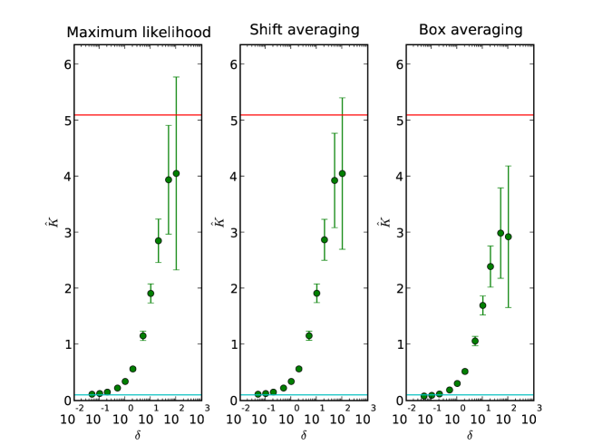
Figure 1: Figure showing statistics for estimators of the eddy diffusivity for the shear flow. The plots show results for various values of the subsampling interval $\delta$ from (left) the maximum likelihood estimator (1.8), (centre) the shift-averaged estimator (4.44), and (right) the box-averaged estimator (4.43). The plots indicate the mean value of the estimators (circular dots), as well as the standard deviation (bars) with statistics computed from 1000 realisations of the Lagrangian trajectory. The correct value $\mathcal{K}=5.1$, and the value of the small-scale diffusivity $\kappa=0.1$ are both indicated as horizontal lines.

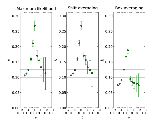
Figure 2: Figure showing statistics for estimators of the eddy diffusivity for the periodically-modulated shear flow with modulation frequency $\omega=1$. The plots show results for various values of the subsampling interval $\delta$ from (left) the maximum likelihood estimator (1.8), (centre) the shift-averaged estimator (4.44), and (right) the box-averaged estimator (4.43). The plots indicate the mean value of the estimators (circular dots), as well as the standard deviation (bars) with statistics computed from 1000 realisations of the Lagrangian trajectory. The correct value $\mathcal{K}=0.125$ (3 d.p.), and the value of the small-scale diffusivity $\kappa=0.1$ are both indicated as horizontal lines.

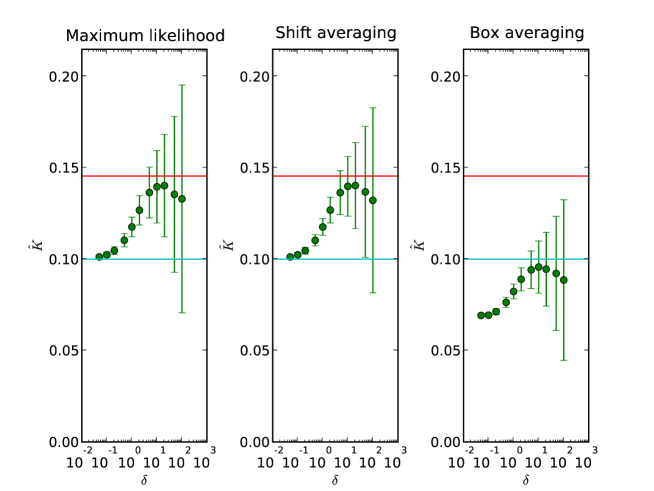
Figure 3: Figure showing statistics for estimators of the eddy diffusivity for the OU-modulated shear flow with parameters $\alpha=1$, $\sigma=0.1$. The plots show results for various values of the subsampling interval $\delta$ from (left) the maximum likelihood estimator (1.8), (centre) the shift-averaged estimator (4.44), and (right) the box-averaged estimator (4.43). The plots indicate the mean value of the estimators (circular dots), as well as the standard deviation (bars) with statistics computed from 1000 realisations of the Lagrangian trajectory. The correct value $\mathcal{K}=0.145$ (3 d.p.), and the value of the small-scale diffusivity $\kappa=0.1$ are both indicated as horizontal lines.

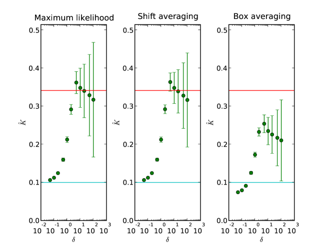
Figure 4: Figure showing statistics for estimators of the eddy diffusivity for the Taylor-Green flow. The plots show results for various values of the subsampling interval $\delta$ from (left) the maximum likelihood estimator (1.8), (centre) the shift-averaged estimator (4.44), and (right) the box-averaged estimator (4.43). The plots indicate the mean value of the estimators (circular dots), as well as the standard deviation (bars) with statistics computed from 1000 realisations of the Lagrangian trajectory. The correct value $\mathcal{K}=0.342$ (3 d.p.), and the value of the small-scale diffusivity $\kappa=0.1$ are both indicated as horizontal lines.

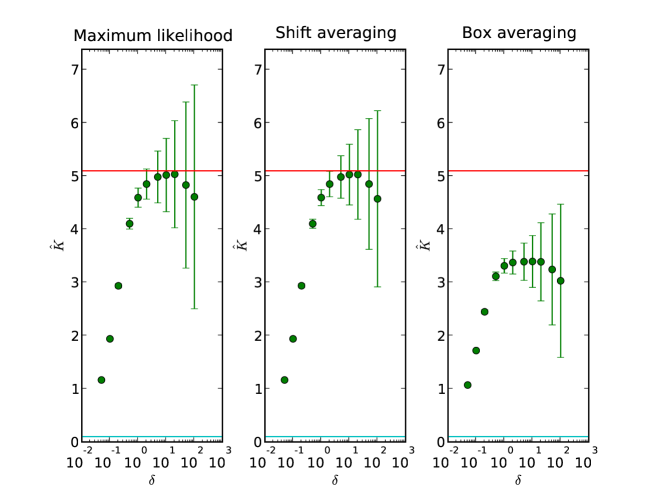
Figure 5: Figure showing statistics for estimators of the eddy diffusivity for the shear flow, applied to the rescaled problem with $\epsilon=0.1$. The plots show results for various values of the subsampling interval $\delta$ from (left) the maximum likelihood estimator (1.8), (center ) the shift-averaged estimator (4.44), and (right) the box-averaged estimator (4.43). The plots indicate the mean value of the estimators (circular dots), as well as the standard deviation (bars) with statistics computed from 1000 realisations of the Lagrangian trajectory. The correct value $\mathcal{K}=5.1$, and the value of the small-scale diffusivity $\kappa=0.1$ are both indicated as horizontal lines.

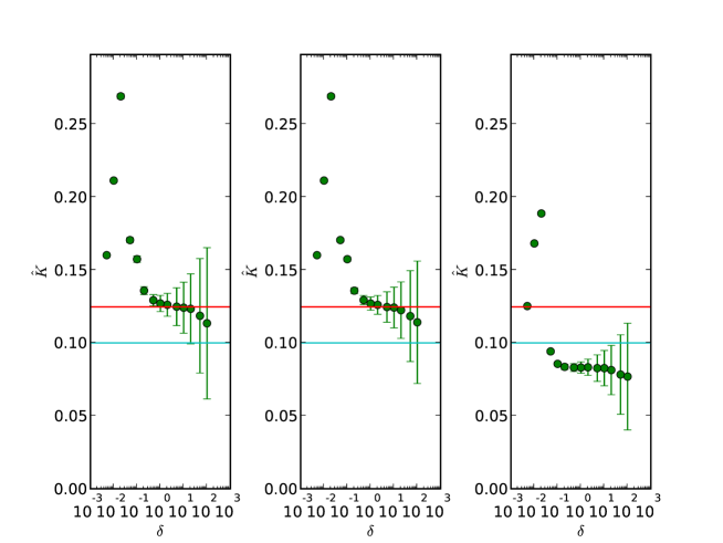
Figure 6: Figure showing statistics for estimators of the eddy diffusivity for the periodically-modulated shear flow with modulation frequency $\omega=1$, applied to the rescaled problem with $\epsilon=0.1$. The plots show results for various values of the subsampling interval $\delta$ from (left) the maximum likelihood estimator (1.8), (centre) the shift-averaged estimator (4.44), and (right) the box-averaged estimator (4.43). The plots indicate the mean value of the estimators (circular dots), as well as the standard deviation (bars) with statistics computed from 1000 realisations of the Lagrangian trajectory. The correct value $\mathcal{K}=0.125$ (3 d.p.), and the value of the small-scale diffusivity $\kappa=0.1$ are both indicated as horizontal lines.

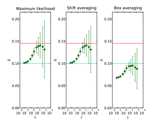
Figure 7: Figure showing statistics for estimators of the eddy diffusivity for the OU-modulated shear flow with parameters $\alpha=1$, $\sigma=0.1$, applied to the rescaled problem with $\epsilon=0.1$. The plots show results for various values of the subsampling interval $\delta$ from (left) the maximum likelihood estimator (1.8), (centre) the shift-averaged estimator (4.44), and (right) the box-averaged estimator (4.43). The plots indicate the mean value of the estimators (circular dots), as well as the standard deviation (bars) with statistics computed from 1000 realisations of the Lagrangian trajectory. The correct value $\mathcal{K}=0.145$ (3 d.p.), and the value of the small-scale diffusivity $\kappa=0.1$ are both indicated as horizontal lines.

Figure 8: Figure showing statistics for estimators of the eddy diffusivity for the Taylor-Green flow, applied to the rescaled problem with $\epsilon=0.1$. The plots show results for various values of the subsampling interval $\delta$ from (left) the maximum likelihood estimator (1.8), (centre) the shift-averaged estimator (4.44), and (right) the box-averaged estimator (4.43). The plots indicate the mean value of the estimators (circular dots), as well as the standard deviation (bars) with statistics computed from 1000 realisations of the Lagrangian trajectory. The correct value $\mathcal{K}=0.342$ (3 d.p.), and the value of the small-scale diffusivity $\kappa=0.1$ are both indicated as horizontal lines.

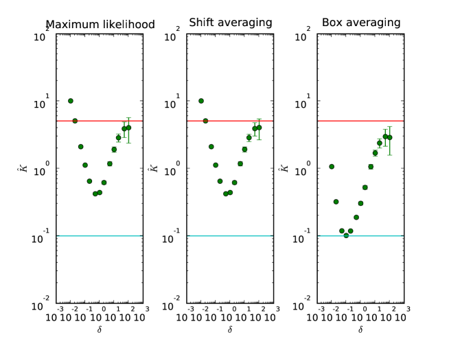
Figure 9: Figure showing statistics for estimators of the eddy diffusivity for the shear flow, where $\mathcal{N}(0,0.1)$ observation noise has been added. The plots show results for various values of the subsampling interval $\delta$ from (left) the maximum likelihood estimator (1.8), (center ) the shift-averaged estimator (4.44), and (right) the box-averaged estimator (4.43). The plots indicate the mean value of the estimators (circular dots), as well as the standard deviation (bars) with statistics computed from 1000 realisations of the Lagrangian trajectory. The correct value $\mathcal{K}=5.1$, and the value of the small-scale diffusivity $\kappa=0.1$ are both indicated as horizontal lines.

Figure 10: Figure showing statistics for estimators of the eddy diffusivity for the periodically-modulated shear flow with modulation frequency $\omega=1$, where $\mathcal{N}(0,0.1)$ observation noise has been added. The plots show results for various values of the subsampling interval $\delta$ from (left) the maximum likelihood estimator (1.8), (centre) the shift-averaged estimator (4.44), and (right) the box-averaged estimator (4.43). The plots indicate the mean value of the estimators (circular dots), as well as the standard deviation (bars) with statistics computed from 1000 realisations of the Lagrangian trajectory. The correct value $\mathcal{K}=0.125$ (3 d.p.), and the value of the small-scale diffusivity $\kappa=0.1$ are both indicated as horizontal lines.

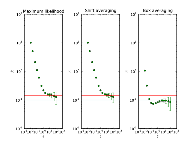
Figure 11: Figure showing statistics for estimators of the eddy diffusivity for the OU-modulated shear flow with parameters $\alpha=1$, $\sigma=0.1$, where $\mathcal{N}(0,0.1)$ observation noise has been added. with $\epsilon=0.1$. The plots show results for various values of the subsampling interval $\delta$ from (left) the maximum likelihood estimator (1.8), (centre) the shift-averaged estimator (4.44), and (right) the box-averaged estimator (4.43). The plots indicate the mean value of the estimators (circular dots), as well as the standard deviation (bars) with statistics computed from 1000 realisations of the Lagrangian trajectory. The correct value $\mathcal{K}=0.145$ (3 d.p.), and the value of the small-scale diffusivity $\kappa=0.1$ are both indicated as horizontal lines.

Figure 12: Figure showing statistics for estimators of the eddy diffusivity for the Taylor-Green flow, where $\mathcal{N}(0,0.1)$ observation noise has been added. The plots show results for various values of the subsampling interval $\delta$ from (left) the maximum likelihood estimator (1.8), (centre) the shift-averaged estimator (4.44), and (right) the box-averaged estimator (4.43). The plots indicate the mean value of the estimators (circular dots), as well as the standard deviation (bars) with statistics computed from 1000 realisations of the Lagrangian trajectory. The correct value $\mathcal{K}=0.342$ (3 d.p.), and the value of the small-scale diffusivity $\kappa=0.1$ are both indicated as horizontal lines.

3.2 The Effect of Observation Error

In this subsection we study the small $\kappa$ asymptotics of the quadratic variation in the presence of observation error. More specifically, we assume that the observed process (along the direction $\xi$) is

$$Y^{\xi}_{t_{j}}=X^{\xi}_{t_{j}}+\theta\epsilon^{\xi}_{t_{j}},\quad j=1,\dots N.$$ (3.34)

The parameter $\theta>0$ measures the strength of the measurement noise which we model through a collection of i.i.d $\mathcal{N}(0,1)$ random variables $\epsilon^{\xi}_{t_{j}}$, which are independent from the Brownian motion driving the Lagrangian dynamics. Since the two sources of noise that appear in the problem are assumed to be independent, the analysis presented in this section also applies to Equation (3.34). In particular, we have that

$$\mathbb{E}\mathcal{K}^{\xi}_{N,\delta}(Y_{t})=\mathbb{E}\left(\mathcal{K}^{\xi}_{N,\delta}(X_{t})\right)+\frac{\theta^{2}}{\delta}.$$

In view of estimate (3.30), we have that

$$\left|\mathbb{E}\left(\mathcal{K}^{\xi}_{N,\delta}(Y_{t})\right)-\mathcal{K}^{\xi}\right|\leq C\kappa^{2\alpha+\frac{1}{2}}\delta^{-\frac{1}{2}}+C\kappa^{2\alpha}\delta^{-1}+\theta^{2}\delta^{-1}.$$

In particular, if $\delta=\kappa^{\gamma}$ with $\gamma<\min(2\alpha,4\alpha+1,0)$ then

$$\lim_{\kappa\rightarrow 0}\big{|}\mathbb{E}\mathcal{K}^{\xi}_{N,\delta}-\mathcal{K}^{\xi}\big{|}=0.$$

We remark that the exponent $\gamma$ is different to the one that appears in the statement of Lemma 3.6, in that it must be negative, irrespective of the scaling of the eddy diffusivity with $\kappa$.

Similarly, in the presence of measurement error, estimate (3.27) has to be modified. It becomes

$$\mathbb{E}\left|\mathcal{K}^{\xi}_{N,\delta}(Y_{t})-\mathcal{K}^{\xi}\right|^{2}=\mathbb{E}\left|\mathcal{K}^{\xi}_{N,\delta}(X_{t})-\mathcal{K}^{\xi}\right|^{2}+3\frac{\theta^{4}}{\delta^{2}}+2\theta^{2}\left(\frac{1}{\delta}+\frac{2}{N\delta}\right)(\mathcal{K}^{\xi}+R),$$ (3.35)

where $R$ is defined in equation (3.31) and estimated in (3.32). We can then use Theorem 3.3 to bound the first term on the right hand side of equation (3.35). Clearly, we require that $\delta\rightarrow\infty$ for the additional terms (which are due to the measurement error) to vanish.

3.3 The Two-Dimensional Shear Flow

In this section we present some results for a particular class of flows for which we can compute the quadratic variation explicitly. The purpose of this is to show that the results obtained in Theorem 3.3 are not sharp.

For two-dimensional flows of the form

$$v(x,y,t)=(0,\eta(t)\sin(x)),$$ (3.36)

where $\eta(t)$ can be either a constant, a periodic function or a stochastic process, we can calculate explicitly the statistics of the quadratic variation of the Lagrangian trajectories [AM90, McL98, MK99]. In the appendix it is shown that for $\eta(t)\equiv 1$, the quadratic variation along the direction of the shear is

$$\mathbb{E}\mathcal{K}_{N,\delta} = \mathcal{K}+\frac{1}{2\kappa^{2}\delta}(e^{-\kappa\delta}-1)+\frac{1}{4\kappa^{2}T}\left(\frac{2}{3}e^{-\kappa\delta}-\frac{1}{6}e^{-4\kappa\delta}-\frac{1}{2}\right)\frac{1-e^{-4\kappa T}}{1-e^{-4\kappa\delta}},$$ (3.37)

where $T=N\delta$ and the effective diffusivity is

$$\mathcal{K}=\kappa+\frac{1}{2\kappa}.$$

From the above formula we immediately deduce that

$$\lim_{\kappa\rightarrow 0}\mathbb{E}\left[\mathcal{K}_{N,\delta}-\mathcal{K}\right]=0$$

provided that

$$\delta=\kappa^{-2-\epsilon}.$$ (3.38)

for $\epsilon>0$, arbitrary. Furthermore, when (3.38) holds, we have that

$$\lim_{\kappa\rightarrow 0}\kappa^{-\epsilon}\left(\mathbb{E}\mathcal{K}_{N,\delta}-\mathcal{K}\right)=-\frac{1}{2}-\frac{1}{8N},$$ (3.39)

the convergence being exponential in $\kappa$.

It is also possible to calculate $\mathbb{E}|\mathcal{K}_{N,\delta}-\mathcal{K}|^{2}$. In particular, we have that

$$\mathbb{E}\left|\mathcal{K}_{N,\delta}-\mathcal{K}\right|^{2} = \frac{1}{N\delta^{2}}\Bigg{(}c_{1}\frac{1}{\kappa^{4}}+c_{2}\delta\frac{1}{\kappa^{3}}+c_{3}{\delta}^{2}\frac{1}{\kappa^{2}}+c_{4}\delta^{2}+$$ (3.40)

$$\qquad\qquad c_{5}\frac{\delta}{\kappa}+c_{6}\kappa^{2}\delta^{2}+c(\delta\kappa)\Bigg{)}$$

$$+\frac{1}{N^{2}\delta^{2}}\Bigg{(}d_{1}\frac{1}{\kappa^{4}}+d_{2}\delta\frac{1}{\kappa^{3}}+d_{3}{\delta}^{2}\frac{1}{\kappa^{2}}+$$

$$\qquad\qquad d_{4}\delta^{2}+d_{5}\frac{\delta}{\kappa}+d_{6}\kappa^{2}\delta^{2}+d(\delta\kappa)\Bigg{)},$$

where the constants $\{c_{i},\,d_{i};i=1,\dots 6\}$ can be calculated explicitly and $c(\delta\kappa),\,d(\delta\kappa)$ converge to a constant exponentially quickly in the limit as $\delta\kappa\rightarrow+\infty$. From the above formula we immediately deduce that

$$\lim_{\kappa\rightarrow 0}\mathbb{E}\left|\mathcal{K}_{N,\delta}-\mathcal{K}\right|^{2}=0$$

provided that (3.38) holds, together with $N\sim\kappa^{-2-\epsilon}$, $\epsilon>0$. Furthermore, under these assumptions on $\delta$ and $N$ we have that

$$\lim_{\kappa\rightarrow 0}\kappa^{-\epsilon}\mathbb{E}\left|\mathcal{K}_{N,\delta}-\mathcal{K}\right|^{2}=\mbox{const}.$$ (3.41)

This example shows that Theorem 3.3 is not sharp. Some details of the calculation of the first two moments of the quadratic variation for the time independent two-dimensional shear flow are presented in Appendix B.

4 Numerical experiments

In this section we illustrate the results of the previous sections with some numerical experiments, and we investigate some modifications to the eddy diffusivity estimator which we shall describe below. The purpose of the numerical experiments that we have performed is to investigate the following issues:

1. The performance of the estimator (1.8) for the eddy diffusivity as a function of the sampling rate for flows with different streamline topologies.

2. Whether an appropriate averaging procedure can reduce the variance of the estimator.

3. The performance of the estimator (1.8) for the eddy diffusivity as a function of the sampling rate for the rescaled problem.

4. The performance of the estimator (1.8) in the presence of measurement noise.

The main conclusions from our numerical experiments can be summarised as follows:

1. The variance of the estimator as well as the optimal sampling rate depend crucially on the streamline topology of the velocity field.

2. Shift averaging (see below) marginally reduces the variance due to multiscale error of the estimator, whereas box averaging (also see below) introduces extra bias into the estimator.

3. There is an optimal sampling rate for the estimator applied to the rescaled problem, but even when using the optimal sampling rate the variance of the estimator can be very large.

4. When the data is subject to measurement noise then subsampling is necessary, even in the absence of multiscale error. Appropriate averaging can reduce the variance due to measurement error.

4.1 The Estimators

We are given a time series of Lagrangian observations of length $T$, sampled at a constant rate $\Delta t$. The number of observations is $N=T/\Delta t$. Our goal is to estimate the eddy diffusivity using the quadratic variation (1.8)

$$\mathcal{K}_{N,\delta}=\frac{1}{2N\delta}\sum_{n=0}^{N-1}\big{(}x_{n+1}-x_{n}\big{)}\otimes\big{(}x_{n+1}-x_{n}\big{)},$$ (4.42)

We will consider both the unrescaled (3.22) as well as the rescaled problems  (2.10). The results presented in Sections (2) and (3) suggest that subsampling at an appropriate rate is necessary in order to estimate the eddy diffusivity correctly, using Lagrangian observations. In the numerical experiments presented in this section we will take the sampling rate to scale either with $\kappa$ (for the unrescaled problem) or with $\epsilon$ (for the rescaled problem), according to the results presented in Theorems 3.3 and (2.1):

$$\delta\sim\kappa^{\alpha},\quad\mbox{or}\quad\delta\sim\epsilon^{\alpha},$$

for some appropriate exponent $\alpha$.

Even if we use (4.42) with $\delta$ chosen optimally, the resulting estimator is clearly not optimal since we are using only a very small portion of the available data. Furthermore, the variance of (1.8) with subsampled data can be enormous, in particular when $\kappa\ll 1$ or $\epsilon\ll 1$. One may attempt to reduce the bias and variance in the estimator by making use of all the data. In particular, it is reasonable to expect that subsampling combined with averaging over the data might lead to a more efficient estimator of the eddy diffusivity with reduced bias in comparison to the estimator (4.42). This methodology was applied in [ASMZ05b, ASMZ05a] in order to estimate the integrated stochastic volatility in the presence of market microstructure noise (observation error).

The most natural way of averaging over the data is by splitting the data into $N_{B}$ bins of size $\delta$ with $\delta N_{B}=N$ and to perform a local averaging over each bin. We use the notation

$$x^{j}_{n}:=x((n-1)\delta+(j-1)\Delta t),\quad n=1,\dots N_{B},\;j=1,\dots J,\quad JN_{B}=N,$$

for the $j$-th observation in the $n$-th bin. $J=\delta/\Delta t$ is the number of observations in each bin. The maximum likelihood estimator (1.8) is then computed using the averaged values

$$\bar{x}_{n}=\frac{1}{J}\sum_{j=1}^{J}x^{j}_{n},$$

leading to the box-averaged estimator:

$$\mathcal{K}_{N_{B},\delta}^{b}=\frac{1}{2N_{B}\delta}\sum_{n=0}^{N_{B}-1}\left(\frac{1}{J}\sum_{j=1}^{J}x^{j}_{n+1}-\frac{1}{J}\sum_{j=1}^{J}x^{j}_{n}\right)\otimes\left(\frac{1}{J}\sum_{j=1}^{J}x^{j}_{n+1}-\frac{1}{J}\sum_{j=1}^{J}x^{j}_{n}\right).$$ (4.43)

A second averaging technique, proposed in [ASMZ05a, ASMZ05b] to remove the effects of market microstructure noise, is to compute a series of estimators, each using a different observation from each bin, and then to compute the average. This is the shift-averaged estimator:

$$\mathcal{K}_{N_{B},\delta}^{s}=\frac{1}{J}\sum_{j=1}^{J}\frac{1}{2N_{B}\delta}\sum_{n=0}^{N_{B}-1}\left(x^{j}_{n+1}-x^{j}_{n}\right)\otimes\left(x^{j}_{n+1}-x^{j}_{n}\right).$$ (4.44)

In all of the tests the box-averaged and shift-averaged estimators were obtained using values from every single timestep. Throughout this section, we only consider the component of the eddy diffusivity along the direction of the shear, since only that component is modified by the flow.

4.2 The Velocity Fields

The numerical experiments were performed using the following four different idealized divergence-free velocity fields in two dimensions:

1. The two-dimensional shear flow:

   $${\bf v}({\bf x})=(0,\sin(x)),$$ (4.45)

   for which the eddy diffusivity is is [MK99]

   $$\mathcal{K}=\kappa+\frac{1}{2\kappa}.$$

2. The periodically-modulated two-dimensional shear flow:

   $${\bf v}({\bf x},t)=(0,\sin(x)\sin(\omega t)),$$ (4.46)

   with $\omega>0$, for which the eddy diffusivity [MBW96] is

   $$\mathcal{K}=\kappa+\frac{1}{4(\omega+\kappa^{2})}.$$

3. The stochastically-modulated two-dimensional shear flow:

   $${\bf v}({\bf x},t)=(0,\eta(t)\sin(x)),$$ (4.47)

   where $\eta(t)$ is an Ornstein-Uhlenbeck process obtained from the equation

   $$\dot{\eta}(t)=-\alpha\eta(t)+\sqrt{2\sigma}\dot{\beta},$$

   and where $\beta$ is a one-dimensional Brownian motion. The eddy diffusivity is

   $$\mathcal{K}=\kappa+\frac{\sigma}{2(\kappa+\alpha)\alpha}.$$ (4.48)

   The calculation of the eddy diffusivity for this velocity field is presented in Appendix A.

4. The Taylor-Green flow:

   $$v(x,t)=\nabla^{\bot}\psi_{TG}(x,y),\quad\psi_{TG}(x,y)=\sin(x)\sin(y).$$ (4.49)

   There is no closed formula for the eddy diffusivity for this flow, but it is well known [CS89, SC90, Chi79, Fan02, Kor04] that the eddy diffusivity is isotropic and that

   $$\mathcal{K}=c^{*}\kappa^{1/2},\quad\kappa\ll 1$$

   with a formula for the prefactor $c^{*}$. For this case we obtain a numerical approximation to the eddy diffusivity $\mathcal{K}$ using the spectral method described in [MM93, Pav02].

We remark that, whereas in the case of the time independent shear flow the eddy diffusivity becomes singular as $\kappa\rightarrow 0$, in all other examples the eddy diffusivity vanishes in the zero molecular diffusion limit. The rate of convergence of $\mathcal{K}$ to $0$ is different for the velocity fields (4.46), (4.47) and the Taylor-Green flow (4.49). From Theorem 3.3 we expect that the different scaling of the eddy diffusivity with $\kappa$ should manifest itself in the scaling of the optimal subsampling rate with $\kappa$.

4.3 Results

Numerical solutions to (1.1) were obtained for each of these cases using the Euler-Maruyama method with a very small timestep to remove the effects of numerical discretisation error. The estimator (1.8) was then computed for each numerical trajectory and compared with the correct value. In the case of the averaged estimators we used all the data in each bin to compute the averages. These calculations were repeated for 1000 realisations of the trajectory with different Brownian motions, and mean and standard deviations for the estimator values were computed.

4.3.1 The Unrescaled Process

Figure 1 shows the results of the three estimators applied to the shear flow for various values of $\delta$ with an interval width $T=1000$, from which the number of bins $N_{B}=T/\delta$ for the averaged estimators can be computed. As is consistent with equation (1.9), the maximum likelihood estimator (1.8) underestimates the eddy diffusivity, and converges to the small-scale diffusivity $\kappa$ for small $\delta$. For larger $\delta$, the mean value of the maximum likelihood estimator approaches the correct value of the eddy diffusivity, but the standard deviation of the estimator becomes large, indicating a large variance which means that the probability of accurately estimating the correct value is small. In comparison, the shift-averaged estimator does not improve the bias by much and the variance is only reduced slightly. The box-averaged estimator increases the bias in the estimator in the sense that it substantially underestimates the eddy diffusivity.

Figure 2 shows the same information for the periodically-modulated shear flow with modulation frequency $\omega$. The small $\delta$ limit is again consistent with equation (1.9), and the mean of the estimator increases to a maximum which is well above the correct value, before decreasing again, with increasing standard-deviations for large values of $\delta$. The shift-averaging again shows very little improvement in either the bias or the variance; the box-averaging reduces the mean towards zero in all cases.

Figure 3 shows the same information for the OU-modulated shear flow with parameters $\alpha=1$, $\sigma=0.1$. The results for the maximum likelihood estimator indicate an optimum value for $\delta$ which corresponds with a maximum of the mean, however the standard deviation increases monotonically with $\delta$. There is a small improvement in the bias and standard deviation for the shift-averaging, and the box-averaging produces a mean which is less than the small-scale diffusivity $\kappa$ for all values of $\delta$.

Figure 4 shows the same information for the Taylor-Green flow. We observe, as is consistent with our theory, that there does seem to be an optimum sampling rate, but the variance is large near the optimal rate, similar to the other cases.

4.3.2 The Rescaled Problem

We then repeated all of these computations for the rescaled problem (2.10) with $\epsilon=0.1$. Figures 5, 6, 7, and 8 show the results for the shear flow, the periodically-modulated shear flow, the OU-modulated shear flow and the Taylor-Green flow respectively. Each of these flows showed that there is an optimal sampling rate for which the mean of the maximum likelihood estimator is close to the correct value, and that the standard deviation is not too large at this sampling rate, although the standard deviation increases for large sampling rates. This illustrates the result of theorem 2.1: the mean of the maximum likelihood estimator converges to the correct value as $\epsilon\to 0$ and the variance converges to zero as the subsampling rate $\delta$ converges to zero.

4.3.3 The Effect of Observation Noise

In this section we consider the combined effect of the multiscale structure and of measurement noise; measurement noise is included using equation (3.34). The experiments of section 4.3.1 were repeated, with $\theta=0.1$. Figures 5, 6, 7, and 8 show the results for the shear flow, the periodically-modulated shear flow, the OU-modulated shear flow and the Taylor-Green flow respectively. These results confirm equation (3.35) in showing that the expectation of the estimators tends to infinity as $\delta$ tends to 0 for non-zero $\theta$. This means that it becomes necessary to subsample even if there is no multiscale error. The results also show that for $\theta=0.1$, the multiscale error dominates the variance of the estimator when subsampling is applied. The shift-averaging technique is effective at removing the variance due to measurement error, but not the variance due to multiscale error.

5 Conclusions

The problem of estimating the eddy diffusivity from noisy Lagrangian observations was studied in this paper. Apart from the direct relevance of our findings to the problem of the accurate parameterisation of the effects of small scales in oceanic models, we believe that this work is also a step towards the development of efficient methods for data-driven coarse graining. Problems similar to the ones considered in this paper have been studied in the context of data assimilation. For example, one might fit data from the full dynamics (i.e. the primitive equations) to the quasi-geostrophic equation which is a reduced model which is obtained from the full dynamics after averaging, in the limit as the Rossby number $Ro$ goes to $0$. Our results suggest that great care has to be taken when fitting data to a reduced model which is not compatible with the data at all scales. This is particularly the case when the reduced model is obtained through a singular limit such as $Ro\rightarrow 0$.

In this paper, we considered this problem for a class of velocity fields (divergence-free, smooth, periodic in space and either steady or modulated in time) for which it can be shown rigorously that a parameterisation of the Lagrangian trajectories exists, in terms of an eddy diffusivity tensor. For this class of flows, it was shown, by means of analysis and numerical experiments, that subsampling is necessary in order to be able to estimate the eddy diffusivity from Lagrangian observations. It was also shown that the optimal sampling rate depends on the topological properties of the velocity field.

Parameter estimation methods that combine subsampling with averaging of the data (defined as shift averaging and box averaging) were also proposed. It was shown that shift averaging is very efficient in reducing the effects of observation error, but only slightly reduces the variance of the estimator. It appears that the shift-averaging technique is only useful for removing measurement error (or microstructure noise in the case of econometrics) and not for reducing the multiscale error, as defined in the introduction. On the other hand, box averaging leads to a biased estimator, even when the optimal sampling rate is used. This should not be surprising, since in the trivial case where the velocity field vanishes (i.e. pure Brownian motion with diffusivity $\kappa$), the expectation of the box averaged estimator is $\kappa/J$ where $J$ is the number of points per bin. On the other hand, for the same problem, the expectation of the shift averaged estimator is $\kappa$.

For efficient accurate coarse graining it is necessary to develop estimators which can deal with the multiscale error more efficiently. Appropriate averaging over the data appears to be an important ingredient of such an estimator. An alternative method has been proposed in [CVE06a] based on the reconstruction of the generator of the observed Markov process; methods that combine subsampling and averaging with this approach are currently being developed.

We believe that our conclusions extend to more general types of velocity fields. For example, one can carry out the analysis and numerical experiments presented in this paper using the class of incompressible Gaussian random velocity fields that were considered in [CC99]. This appears to be a general class of models to consider since one can obtain velocity fields with any chosen energy spectrum. The regularity of such velocity fields should definitely play an important role in the statistical inference procedure.

Clearly the calculation of the optimal sampling rate from the data is crucial for our approach. It appears that frequency domain techniques are more suitable for addressing this issue, and this will be investigated in subsequent publications.

Acknowledgements. The authors are particularly grateful to A.M. Stuart and P.R. Kramer for their very careful reading of an earlier draft of the paper and for many useful suggestions and comments.

Appendix A Derivation of Formula (4.48)

In this appendix we derive the formula for the effective diffusivity for the OU-modulated shear flow (4.47). Homogenization problems for Gaussian incompressible velocity fields that are given in terms of an Ornstein-Uhlenbeck process have been considered in [CX97, PSZ07]. The results presented in these papers imply that

$$\lim_{\epsilon\rightarrow 0}\epsilon y(t/\epsilon^{2})=\sqrt{2\mathcal{K}}W(t),$$

weakly on $C([0,T];\mathbb{R})$ where $W(t)$ is a standard one-dimensional Brownian motion and

$$\mathcal{K}=\kappa+\kappa\|\partial_{x}\phi\|^{2}_{L^{2}(X;\rho)}+\sigma\|\partial_{\eta}\phi\|^{2}_{L^{2}(X;\rho)}.$$ (1.50)

We have used the notation $X:=(2\pi\mathbb{T})^{2}\times\mathbb{R}$, and $\phi$ and $\rho$ are the unique solutions of the equations

$$-\mathcal{L}\phi=\eta\sin(x),\quad\int_{X}\phi\rho\,dX=0,$$ (1.51a)

$$-\mathcal{L}^{*}\rho=0,\quad\int_{X}\rho\,dX=1.$$ (1.51b)

We have used the notation $dX=dxdyd\eta$ and $\mathcal{L}$ is the generator of the Markov process restricted on $X$:

$$\mathcal{L}=\eta\sin(x)\partial_{y}+\kappa\partial_{x}^{2}+\kappa\partial_{y}^{2}-\alpha\eta\partial_{\eta}+\sigma\partial_{\eta}^{2}.$$

$\mathcal{L}^{*}$ denotes the $L^{2}(X)$-adjoint, i.e. the Fokker-Planck operator. We can easily solve equations (1.51a) and (1.51b) to obtain

$$\rho\,dxdyd\eta=\frac{1}{Z}e^{-\frac{\alpha\eta^{2}}{2\sigma^{2}}}\,dxdyd\eta,\quad Z=4\pi^{2}\sqrt{\frac{2\pi\sigma}{\alpha}}$$

and

$$\phi(x,y,\eta)=\frac{1}{\kappa+\alpha}\eta\sin(x).$$

Consequently:

$$\|\partial_{x}\phi\|_{(L^{2};\rho)}^{2} = \frac{1}{(\kappa+\alpha)^{2}}Z^{-1}\int_{X}\eta^{2}(\cos(x))^{2}\rho\,dX$$

$$= \frac{\sigma}{2\alpha}\frac{1}{(\kappa+\alpha)^{2}}$$

and

$$\|\partial_{\eta}\phi\|_{(L^{2};\rho)}^{2} = \frac{1}{(\kappa+\alpha)^{2}}Z^{-1}\int_{X}(\sin(x))^{2}\rho\,dX$$

$$= \frac{1}{2(\kappa+\alpha)^{2}}.$$

Upon inserting the above two formulas in (1.50) we obtain (4.48).

Appendix B The two-dimensional shear flow

In this appendix we study in more detail the problem of estimating the eddy diffusivity from Lagrangian observations for a class of two-dimensional shear flows. Throughout this appendix we only consider the eddy diffusivity along the direction of the shear. The flows that we will consider are of the form

$$v(x,y,t)=(0,\eta(t)f(x)),$$ (2.52)

where $f(x)$ is a smooth periodic function and $\eta(t)$ is either a constant, a smooth periodic function of time or a stochastic process, e.g. the Onrstein-Uhlenbeck process

$$\frac{d\eta}{dt}=-\alpha\eta+\sqrt{2\sigma}\frac{dW}{dt}.$$

As it has already been noted in [AM90, McL98, MK99], for this class of velocity fields the Lagrangian equations can be solved explicitly. In particular, we have that

$$y(t)=y(0)+\int_{0}^{t}\eta(s)f(x(0)+\sqrt{2\kappa}W_{1}(s))\,ds+\sqrt{2\kappa}\,W_{2}(t),$$ (2.53)

where $W_{1}(t)$ and $W_{2}(t)$ are one dimensional independent Brownian motions. Hence, the formula for the quadratic variation becomes

$$\mathcal{K}_{N,\delta}=\frac{1}{2N\delta}\sum_{n=0}^{N-1}\left(\int_{n\delta}^{(n+1)\delta}\eta(s)f(x(0)+\sqrt{2\kappa}W_{1}(s))\,ds+\sqrt{2\kappa}\Delta W_{2}(n\delta)\right)^{2},$$ (2.54)

where $\Delta W_{2}(n\delta)=W_{2}((n+1)\delta)-W_{2}(n\delta)$. Since $f(x)$ is a periodic function, the calculation of the statistics of the quadratic variation can be accomplished by calculating the statistics of integrals of trigonometric functions of the Brownian motion. This calculation can be done by using properties of integrals of symmetric functions, that is functions $f:[n\delta,(n+1)\delta]^{d}\mapsto\mathbb{R}$ for which $f(t_{\sigma_{1}},t_{\sigma_{2}},\dots t_{\sigma_{d}})=f(t_{1},t_{2},\dots t_{d})$ for all permutations $\sigma$ of $(1,2,\dots d)$. In this way, we can calculate the quadratic variation as a function of $\kappa$ and $\delta$ in an explicit form. For simplicity we will consider the case $\eta(t)\equiv 1$, $f(x)=\sin(x)$ and $x(0)=y(0)=0$. The general case can be treated similarly.

For the velocity field

$$v(x,y)=(0,\sin(x))$$

We can calculate the expectation of the 22-component of the quadratic variation equation (3.37), and hence prove (3.39). Since $W_{1}(t)$ and $W_{2}(t)$ are independent, we immediately deduce that

$$\mathbb{E}\left[(y_{n+1}-y_{n})^{2}\right] = \int_{n\delta}^{(n+1)\delta}\int_{n\delta}^{(n+1)\delta}\mathbb{E}\left[\sin(\sqrt{2\kappa}W_{1}(s_{1}))\sin(\sqrt{2\kappa}W_{1}(s_{2}))\right]\operatorname{d}s_{2}\operatorname{d}s_{1}+2\kappa\delta.$$

In order to calculate the integral on the right hand side of the above equation (which we denote by $S$), we use trigonometric identities together with the formula for the expectation of the characteristic function of a Gaussian random variable to obtain

$$S = -\frac{1}{4}\sum_{\boldsymbol{a}\in I}a_{1}a_{2}\int_{n\delta}^{(n+1)\delta}\int_{n\delta}^{(n+1)\delta}\mathbb{E}\left[e^{i\sqrt{2\kappa}\left(a_{1}W_{1}(s_{1})+a_{2}W_{1}(s_{2})\right)}\right]\operatorname{d}s_{2}\operatorname{d}s_{1}$$

$$= -\frac{1}{4}\sum_{\boldsymbol{a}\in I}a_{1}a_{2}\int_{n\delta}^{(n+1)\delta}\int_{n\delta}^{(n+1)\delta}e^{-2\kappa\delta\sum_{i,j=1}^{2}a_{i}a_{j}\min(s_{i},s_{j})}\operatorname{d}s_{2}\operatorname{d}s_{1},$$

where $\boldsymbol{a}=(a_{1},a_{2})$ and $I$ is the index set $\{-1,1\}\times\{-1,1\}=\{-1,1\}^{2}$. The integrand is symmetric in $s_{1}$ and $s_{2}$, and, using properties of multiple integrals of symmetric functions, we can write the above integral in the form

$$S = -\frac{1}{8}\sum_{\boldsymbol{a}\in I}a_{1}a_{2}\int_{n\delta}^{(n+1)\delta}\int_{s_{1}}^{(n+1)\delta}e^{-2\kappa\delta\sum_{i=1}^{2}s_{i}(a_{i}^{2}+\sum_{i<j}a_{i}a_{j})}\operatorname{d}s_{2}\operatorname{d}s_{1}.$$

Evaluating this formula using Maple gives

$$S=2\kappa\delta+\frac{\delta}{\kappa}+\frac{1}{2\kappa^{2}}\Bigg{(}-\frac{1}{6}e^{-4\kappa(n+1)\delta}-\frac{1}{2}e^{-4\kappa n\delta}+\frac{2}{3}e^{-\kappa(4n+1)\delta}+2e^{-\kappa\delta}-2\Bigg{)},$$ (2.55)

from which (3.37) follows upon summation.

We can also calculate $\mathbb{E}\left|\mathcal{K}_{N,\delta}-\mathcal{K}\right|^{2}$, leading to equation (3.40), and hence (3.41). We have

$$\mathbb{E}\left|\mathcal{K}_{N,\delta}-\mathcal{K}\right|^{2}=\mathbb{E}\left|\mathcal{K}_{N,\delta}\right|^{2}-2\mathbb{E}\left(\mathcal{K}_{N,\delta}\right)\left(\kappa+\frac{1}{2\kappa}\right)+\left(\kappa+\frac{1}{2\kappa}\right)^{2}.$$ (2.56)

We have already calculated the expectation of the quadratic variation, and it remains to compute the second moment. We have

$$\mathbb{E}\left|\mathcal{K}_{\delta}\right|^{2} = \frac{1}{4N^{2}\delta^{2}}\sum_{n=1}^{N}\sum_{m=1}^{N}\mathbb{E}\left((y^{n}-y^{n-1})^{2}(y^{m}-y^{m-1})^{2}\right)$$

$$= \frac{1}{4N^{2}\delta^{2}}\sum_{n=1}^{N}\underbrace{\mathbb{E}\left[(y^{n}-y^{n-1})^{4}\right]}_{=S_{1}^{n}}+\frac{1}{2N^{2}\delta^{2}}\sum_{n=1}^{N}\sum_{m<n}\underbrace{\mathbb{E}\left[(y^{n}-y^{n-1})^{2}(y^{m}-y^{m-1})^{2}\right]}_{=S_{2}^{nm}}.$$

We shall separately compute these two types of terms, namely the diagonal terms $S_{1}^{n}$ and the off-diagonal terms $S_{2}^{nm}$.

First we compute $S_{1}^{n}$.

$$S_{1}^{n} = \underbrace{\mathbb{E}\left[\left(\int_{n\delta}^{(n+1)\delta}\sin(\sqrt{2\kappa}W_{1}(s))\operatorname{d}{s}\right)^{4}\right]}_{S_{11}^{n}}$$

$$+12\kappa\delta\left(\frac{\delta}{\kappa}+\frac{1}{2\kappa^{2}}\Bigg{(}-\frac{1}{6}e^{-4\kappa(n+1)\delta}-\frac{1}{2}e^{-4\kappa n\delta}+\frac{2}{3}e^{-\kappa(4n+1)\delta}+2e^{-\kappa\delta}-2\Bigg{)}\right)$$

$$+12\kappa^{2}\delta^{2},$$

where (2.55) has been used. For the calculation of $S_{11}^{n}$ we use trigonometric identities, together with the formula for the expectation of the characteristic function of a Gaussian random variable to obtain

$$S_{11}^{n} = \frac{1}{16}\sum_{\boldsymbol{a}\in I}\prod_{k=1}^{4}a_{k}\int_{s_{k}=n\delta}^{(n+1)\delta}e^{-2\kappa\sum_{i,j=1}^{4}a_{i}a_{j}\min(s_{i},s_{j})}\operatorname{d}{s}_{k},$$

where $\boldsymbol{a}=(a_{1},a_{2},a_{3},a_{4})$ and $I$ is the indexing set $\{-1,1\}^{4}$. The integrand in this multiple integral is a symmetric function, and hence we may write

$$S_{11}^{n} = \frac{3}{2}\sum_{\boldsymbol{a}\in I}\prod_{k=1}^{4}a_{k}\int_{s_{1}=n\delta}^{(n+1)\delta}\int_{s_{2}=s_{1}}^{(n+1)\delta}\int_{s_{3}=s_{2}}^{(n+1)\delta}\int_{s_{4}=s_{3}}^{(n+1)\delta}e^{-2\kappa\sum_{i,j=1}^{4}a_{i}a_{j}\min(s_{i},s_{j})}\operatorname{d}{s}_{1}\operatorname{d}{s}_{2}\operatorname{d}{s}_{3}\operatorname{d}{s}_{4}.$$

This can be computed using Maple:

$$S_{11}^{n} = {\frac{1}{26880}}\,{\frac{1}{{\kappa}^{4}\left({e^{\kappa\,n\delta}}\right)^{16}\left({e^{\kappa\,\delta}}\right)^{16}}}$$

$$\;+{\frac{261}{64}}\,{\kappa}^{-4}+{\frac{1}{960}}\,{\frac{1}{\left({e^{\kappa\,n\delta}}\right)^{16}{\kappa}^{4}\left({e^{\kappa\,\delta}}\right)^{4}}}-{\frac{1}{3360}}\,{\frac{1}{\left({e^{\kappa\,n\delta}}\right)^{16}{\kappa}^{4}\left({e^{\kappa\,\delta}}\right)^{9}}}-{\frac{45}{16}}\,{\frac{\delta}{{\kappa}^{3}}}$$

$$\;-{\frac{49}{12}}\,{\frac{1}{{\kappa}^{4}{e^{\kappa\,\delta}}}}-{\frac{1}{2400}}\,{\frac{1}{{\kappa}^{4}\left({e^{\kappa\,n\delta}}\right)^{4}\left({e^{\kappa\,\delta}}\right)^{9}}}+{\frac{1}{120}}\,{\frac{\delta}{{\kappa}^{3}\left({e^{\kappa\,n\delta}}\right)^{4}\left({e^{\kappa\,\delta}}\right)^{4}}}$$

$$\;+{\frac{19}{24}}\,{\frac{1}{{\kappa}^{4}\left({e^{\kappa\,n\delta}}\right)^{4}}}-{\frac{1}{480}}\,{\frac{1}{\left({e^{\kappa\,n\delta}}\right)^{16}{\kappa}^{4}{e^{\kappa\,\delta}}}}-{\frac{229}{288}}\,{\frac{1}{{\kappa}^{4}\left({e^{\kappa\,n\delta}}\right)^{4}{e^{\kappa\,\delta}}}}$$

$$\;-5/4\,{\frac{\delta}{{\kappa}^{3}{e^{\kappa\,\delta}}}}+3/4\,{\frac{{\delta}^{2}}{{\kappa}^{2}}}+{\frac{1}{192}}\,{\frac{1}{{\kappa}^{4}\left({e^{\kappa\,\delta}}\right)^{4}}}$$

$$\;-{\frac{5}{12}}\,{\frac{\delta}{{\kappa}^{3}\left({e^{\kappa\,n\delta}}\right)^{4}{e^{\kappa\,\delta}}}}-3/8\,{\frac{\delta}{{\kappa}^{3}\left({e^{\kappa\,n\delta}}\right)^{4}}}+{\frac{7}{1800}}\,{\frac{1}{{\kappa}^{4}\left({e^{\kappa\,n\delta}}\right)^{4}\left({e^{\kappa\,\delta}}\right)^{4}}}+{\frac{1}{768}}\,{\frac{1}{\left({e^{\kappa\,n\delta}}\right)^{16}{\kappa}^{4}}}$$

After summation, all the terms containing exponentials given rise to terms which converge to a constant divided by $\delta^{2}N^{2}$ faster than any polynomial power of $\delta\kappa$ as $\kappa\delta\to\infty$.

Next we compute $S_{2}$. Since $n<m$, the term inside the sum is

$$\mathbb{E}\left[(y^{n+1}-y^{n})^{2}(y^{m+1}-y^{m})^{2}\right] = \mathbb{E}\Bigg{[}\left(\int_{n\delta}^{(n+1)\delta}\sin(\sqrt{2\kappa}W_{1}(s))\operatorname{d}{s}+\sqrt{2\kappa}\int_{n\delta}^{(n+1)\delta}\operatorname{d}{W_{2}}(s)\right)^{2}$$

$$\quad\times\left(\int_{m\delta}^{(m+1)\delta}\sin(\sqrt{2\kappa}W_{1}(s))\operatorname{d}{s}+\sqrt{2\kappa}\int_{m\delta}^{(m+1)\delta}\operatorname{d}{W_{2}}(s)\right)^{2}\Bigg{]}$$

$$= \underbrace{\mathbb{E}\Bigg{[}\left(\int_{n\delta}^{(n+1)\delta}\sin(\sqrt{2\kappa}W_{1}(s))\operatorname{d}{s}\right)^{2}\left(\int_{m\delta}^{(m+1)\delta}\sin(\sqrt{2\kappa}W_{1}(s))\operatorname{d}{s}\right)^{2}\Bigg{]}}_{S_{21}^{nm}}$$

$$+2\kappa\delta\Bigg{(}2\kappa\delta+\frac{\delta}{\kappa}+\frac{1}{2\kappa^{2}}\Bigg{(}-\frac{1}{6}e^{-4\kappa(m+1)\delta}-\frac{1}{2}e^{-4\kappa m\delta}+$$

$$\qquad\qquad\qquad\qquad\qquad\qquad\qquad\frac{2}{3}e^{-\kappa(4m+1)\delta}+2e^{-\kappa\delta}-2\Bigg{)}\Bigg{)}$$

$$+2\kappa\delta\Bigg{(}2\kappa\delta+\frac{\delta}{\kappa}+\frac{1}{2\kappa^{2}}\Bigg{(}-\frac{1}{6}e^{-4\kappa(n+1)\delta}-\frac{1}{2}e^{-4\kappa n\delta}+$$

$$\qquad\qquad\qquad\qquad\qquad\qquad\qquad\frac{2}{3}e^{-\kappa(4n+1)\delta}+2e^{-\kappa\delta}-2\Bigg{)}\Bigg{)}$$

$$\quad+4\kappa^{2}\delta^{2},$$

where (2.55) has been used again. A similar calculation to that for $S_{11}^{n}$, making use of the fact that $m>n$ gives

$$S_{21}^{nm} = \int_{s_{1}=n\delta}^{(n+1)\delta}\int_{s_{2}=n\delta}^{(n+1)\delta}\frac{1}{16}\sum_{\boldsymbol{a}\in I}\left(\prod_{k=1}^{4}a_{k}\right)e^{-2\kappa\left(\sum_{i,j=1}^{2}a_{i}a_{j}\min(s_{i},s_{j})+2\sum_{i=1}^{2}\sum_{j=3}^{4}a_{i}a_{j}s_{i}\right)}$$

$$\qquad\times\int_{s_{3}=m\delta}^{(m+1)\delta}\int_{s_{4}=m\delta}^{(m+1)\delta}e^{-2\kappa\sum_{i,j=3}^{4}a_{i}a_{j}\min(s_{i},s_{j})}\operatorname{d}{s}_{1}\operatorname{d}{s}_{2}\operatorname{d}{s}_{3}\operatorname{d}{s}_{4}.$$

The integrand for the two inner integrals, and the integrand for the two outer integrals are both symmetric functions, and we obtain

$$S_{21}^{nm} = \frac{1}{4}\int_{s_{1}=n\delta}^{(n+1)\delta}\int_{s_{2}=s_{1}}^{(n+1)\delta}\sum_{\boldsymbol{a}\in I}\left(\prod_{k=1}^{4}a_{k}\right)e^{-2\kappa\left(\sum_{i=1}^{2}s_{i}\left(a_{i}^{2}+2\sum_{i<j<3}a_{i}a_{j}\right)+2\sum_{i=1}^{2}\sum_{j=3}^{4}a_{i}a_{j}s_{i}\right)}$$

$$\qquad\times\int_{s_{3}=m\delta}^{(m+1)\delta}\int_{s_{4}=s3}^{(m+1)\delta}e^{-2\kappa\sum_{i=3}^{4}s_{i}\left(a_{i}^{2}+2\sum_{i<j}a_{i}a_{j}\right)}\operatorname{d}{s}_{1}\operatorname{d}{s}_{2}\operatorname{d}{s}_{3}\operatorname{d}{s}_{4}.$$

This can be computing using Maple:

$$S_{21}^{nm} = -2\,{\frac{1}{{\kappa}^{4}{e^{\delta\,\kappa}}}}+{\frac{1}{2016}}\,{\frac{1}{{\kappa}^{4}\left({e^{\kappa\,m\delta}}\right)^{4}\left({e^{\delta\,\kappa}}\right)^{16}\left({e^{\kappa\,n\delta}}\right)^{12}}}+{\frac{1}{210}}\,{\frac{1}{{\kappa}^{4}\left({e^{\kappa\,m\delta}}\right)^{4}\left({e^{\delta\,\kappa}}\right)^{6}\left({e^{\kappa\,n\delta}}\right)^{12}}}$$

$$\;-{\frac{1}{504}}\,{\frac{1}{{\kappa}^{4}\left({e^{\kappa\,m\delta}}\right)^{4}\left({e^{\delta\,\kappa}}\right)^{13}\left({e^{\kappa\,n\delta}}\right)^{12}}}$$

$$\;+{\frac{1}{1440}}\,{\frac{1}{{\kappa}^{4}\left({e^{\kappa\,m\delta}}\right)^{4}\left({e^{\delta\,\kappa}}\right)^{4}\left({e^{\kappa\,n\delta}}\right)^{12}}}-{\frac{1}{840}}\,{\frac{1}{{\kappa}^{4}\left({e^{\kappa\,m\delta}}\right)^{4}\left({e^{\delta\,\kappa}}\right)^{9}\left({e^{\kappa\,n\delta}}\right)^{12}}}-1/12\,{\frac{1}{{\kappa}^{4}\left({e^{\delta\,\kappa}}\right)^{5}\left({e^{\kappa\,n\delta}}\right)^{4}}}$$

$$\;+{\frac{1}{60}}\,{\frac{\delta}{{\kappa}^{3}\left({e^{\kappa\,m\delta}}\right)^{4}}}-1/45\,{\frac{\delta}{{\kappa}^{3}\left({e^{\kappa\,m\delta}}\right)^{4}{e^{\delta\,\kappa}}}}+{\frac{1}{180}}\,{\frac{\delta}{{\kappa}^{3}\left({e^{\kappa\,m\delta}}\right)^{4}\left({e^{\delta\,\kappa}}\right)^{4}}}+1/48\,{\frac{\left({e^{\kappa\,n\delta}}\right)^{4}}{{\kappa}^{4}\left({e^{\kappa\,m\delta}}\right)^{4}}}+$$

$$\;{\frac{17}{2700}}\,{\frac{1}{{\kappa}^{4}\left({e^{\kappa\,m\delta}}\right)^{4}\left({e^{\delta\,\kappa}}\right)^{4}}}-{\frac{1}{600}}\,{\frac{1}{{\kappa}^{4}\left({e^{\kappa\,m\delta}}\right)^{4}\left({e^{\delta\,\kappa}}\right)^{9}}}+1/4\,{\frac{1}{{\kappa}^{4}\left({e^{\kappa\,n\delta}}\right)^{4}}}-{\frac{7}{12}}\,{\frac{1}{{\kappa}^{4}{e^{\delta\,\kappa}}\left({e^{\kappa\,n\delta}}\right)^{4}}}$$

$$\;-1/12\,{\frac{\left({e^{\kappa\,n\delta}}\right)^{4}\left({e^{\delta\,\kappa}}\right)^{3}}{{\kappa}^{4}\left({e^{\kappa\,m\delta}}\right)^{4}}}+$$

$$\;1/32\,{\frac{\left({e^{\kappa\,n\delta}}\right)^{4}\left({e^{\delta\,\kappa}}\right)^{4}}{{\kappa}^{4}\left({e^{\kappa\,m\delta}}\right)^{4}}}-1/36\,{\frac{\left({e^{\kappa\,n\delta}}\right)^{4}}{{\kappa}^{4}\left({e^{\kappa\,m\delta}}\right)^{4}{e^{\delta\,\kappa}}}}+1/18\,{\frac{\left({e^{\delta\,\kappa}}\right)^{2}\left({e^{\kappa\,n\delta}}\right)^{4}}{{\kappa}^{4}\left({e^{\kappa\,m\delta}}\right)^{4}}}$$

$$\;+{\frac{1}{288}}\,{\frac{\left({e^{\kappa\,n\delta}}\right)^{4}}{{\kappa}^{4}\left({e^{\kappa\,m\delta}}\right)^{4}\left({e^{\delta\,\kappa}}\right)^{4}}}-1/4\,{\frac{\delta}{{\kappa}^{3}\left({e^{\kappa\,n\delta}}\right)^{4}}}+1/3\,{\frac{\delta}{{\kappa}^{3}{e^{\delta\,\kappa}}\left({e^{\kappa\,n\delta}}\right)^{4}}}-1/12\,{\frac{\delta}{{\kappa}^{3}\left({e^{\delta\,\kappa}}\right)^{4}\left({e^{\kappa\,n\delta}}\right)^{4}}}$$

$$\;+1/12\,{\frac{1}{{\kappa}^{4}\left({e^{\delta\,\kappa}}\right)^{4}\left({e^{\kappa\,n\delta}}\right)^{4}}}+1/3\,{\frac{1}{{\kappa}^{4}\left({e^{\delta\,\kappa}}\right)^{2}\left({e^{\kappa\,n\delta}}\right)^{4}}}+{\frac{1}{{\kappa}^{4}\left({e^{\delta\,\kappa}}\right)^{2}}}+2\,{\frac{\delta}{{\kappa}^{3}{e^{\delta\,\kappa}}}}$$

$$\;+{\frac{{\delta}^{2}}{{\kappa}^{2}}}-2\,{\frac{\delta}{{\kappa}^{3}}}+{\kappa}^{-4}-{\frac{1}{360}}\,{\frac{1}{{\kappa}^{4}\left({e^{\kappa\,m\delta}}\right)^{4}{e^{\delta\,\kappa}}\left({e^{\kappa\,n\delta}}\right)^{12}}}$$

$$\;+{\frac{1}{480}}\,{\frac{1}{{\kappa}^{4}\left({e^{\kappa\,m\delta}}\right)^{4}\left({e^{\kappa\,n\delta}}\right)^{12}}}-{\frac{1}{280}}\,{\frac{1}{{\kappa}^{4}\left({e^{\kappa\,m\delta}}\right)^{4}\left({e^{\delta\,\kappa}}\right)^{5}\left({e^{\kappa\,n\delta}}\right)^{12}}}$$

$$\;+{\frac{1}{672}}\,{\frac{1}{{\kappa}^{4}\left({e^{\kappa\,m\delta}}\right)^{4}\left({e^{\delta\,\kappa}}\right)^{12}\left({e^{\kappa\,n\delta}}\right)^{12}}}+{\frac{17}{900}}\,{\frac{1}{{\kappa}^{4}\left({e^{\kappa\,m\delta}}\right)^{4}}}$$

$$\;-{\frac{1}{72}}\,{\frac{\left({e^{\delta\,\kappa}}\right)^{3}}{{\kappa}^{4}\left({e^{\kappa\,m\delta}}\right)^{4}}}-{\frac{161}{5400}}\,{\frac{1}{{\kappa}^{4}\left({e^{\kappa\,m\delta}}\right)^{4}{e^{\delta\,\kappa}}}}+{\frac{1}{54}}\,{\frac{\left({e^{\delta\,\kappa}}\right)^{2}}{{\kappa}^{4}\left({e^{\kappa\,m\delta}}\right)^{4}}}$$

$$\;-{\frac{1}{200}}\,{\frac{1}{{\kappa}^{4}\left({e^{\kappa\,m\delta}}\right)^{4}\left({e^{\delta\,\kappa}}\right)^{5}}}+{\frac{1}{150}}\,{\frac{1}{{\kappa}^{4}\left({e^{\kappa\,m\delta}}\right)^{4}\left({e^{\delta\,\kappa}}\right)^{6}}}.$$

After the double summation, all the terms containing exponentials given rise to terms which converge to a constant multiplied by $(N-1)/\delta^{2}N^{2}$ faster than any polynomial power of $\delta\kappa$ as $\kappa\delta\to\infty$.

Collecting terms

$$\mathbb{E}\left|\mathcal{K}_{N,\delta}\right|^{2} = \frac{1}{4\kappa^{2}\delta^{2}}-\frac{1}{2\kappa^{3}\delta}+\frac{1}{4\kappa^{2}}+1-\frac{1}{\kappa\delta}+\kappa^{2}$$

$$+\frac{1}{N\delta^{2}}\left(c_{1}\frac{1}{\kappa^{4}}+c_{2}\delta\frac{1}{\kappa^{3}}+c_{3}{\delta}^{2}\frac{1}{\kappa^{2}}+c_{4}\delta^{2}+c_{5}\frac{\delta}{\kappa}+c_{6}\kappa^{2}\delta^{2}+c(\delta\kappa)\right)$$

$$+\frac{1}{N^{2}\delta^{2}}\left(d_{1}\frac{1}{\kappa^{4}}+d_{2}\delta\frac{1}{\kappa^{3}}+d_{3}{\delta}^{2}\frac{1}{\kappa^{2}}+d_{4}\delta^{2}+d_{5}\frac{\delta}{\kappa}+d_{6}\kappa^{2}\delta^{2}+d(\delta\kappa)\right),$$

where the constants $\{c_{i},\,d_{i};i=1,\dots 6\}$ can be read from the above formulas and $c(\delta\kappa),\,d(\delta\kappa)$ converge exponentially fast to a constant in the limit $\delta\kappa\rightarrow+\infty$.

Upon computing the remaining terms in equation (2.56) we notice that all leading order terms are cancelled and we end up with

$$\mathbb{E}\left|\mathcal{K}_{N,\delta}-\mathcal{K}\right|^{2} = \frac{1}{N\delta^{2}}\left(c_{1}\frac{1}{\kappa^{4}}+c_{2}\delta\frac{1}{\kappa^{3}}+c_{3}{\delta}^{2}\frac{1}{\kappa^{2}}+c_{4}\delta^{2}+c_{5}\frac{\delta}{\kappa}+c_{6}\kappa^{2}\delta^{2}+c(\delta\kappa)\right)$$

$$+\frac{1}{N^{2}\delta^{2}}\left(d_{1}\frac{1}{\kappa^{4}}+d_{2}\delta\frac{1}{\kappa^{3}}+d_{3}{\delta}^{2}\frac{1}{\kappa^{2}}+d_{4}\delta^{2}+d_{5}\frac{\delta}{\kappa}+d_{6}\kappa^{2}\delta^{2}+d(\delta\kappa)\right),$$

which is precisely equation (3.40).

References

- [ASMZ05a] Y. Ait-Sahalia, P. A. Mykland, and L Zhang. How often to sample a continuous-time process in the presence of market microstructure noise. Rev. Financ. Studies, 18:351–416, 2005.
- [ASMZ05b] Y. Ait-Sahalia, P. A. Mykland, and L Zhang. A tale of two time scales: Determining integrated volatility with noisy high-frequency data. J. Amer. Stat. Assoc., 100:1394–1411, 2005.
- [AM90] M. Avellaneda and A. J. Majda, Mathematical models with exact renormalization for turbulent transport, Comm. Pure Appl. Math., 131 (1990), pp. 381–429.
- [AM91] M. Avellaneda and A. J. Majda, An integral representation and bounds on the effective diffusivity in passive advection by laminar and turbulent flows, Comm. Math. Phys., 138 (1991), pp. 339–391.
- [BSGMO98] S. Bauer, M. S. Swenson, A. Griffa, A. J. Mariano, and K. Owens, Eddy-mean flow decomposition and eddy-diffusivity estimates in the tropical pacific ocean. 1. Methodology, J. Geophys. Res., 103 (1998), pp. 30855–30871.
- [BSG02] S. Bauer, M. S. Swenson, and A. Griffa, Eddy mean flow decomposition and eddy diffusivity estimates in the tropical Pacific Ocean: 2. Results, J. Geophys. Res., 107 (2002), p. 3154. doi:10.1029/2000JC000613.
- [Bat99] R. Battacharya. Multiscale diffusion processes with periodic coefficients and an application to solute transport in porous media. The Annals of Applied Probability, 9(4):951–1020, 1999.
- [BGW89] R. N. Bhattacharya, V.K. Gupta, and H.F. Walker. Asymptotics of solute dispersion in periodic porous media. SIAM J. APPL. MATH, 49(1):86–98, 1989.
- [BLP78] A. Bensoussan, J.-L. Lions, and G. Papanicolaou. Asymptotic analysis for periodic structures, volume 5 of Studies in Mathematics and its Applications. North-Holland Publishing Co., Amsterdam, 1978.
- [BM02] P. S. Berloff and J.C. McWilliams. Material transport in oceanic gyres. Part II: Hierarchy of stochastic models. J. Phys. Oceanogr., 32:797–830, 2002.
- [BM03] P. S. Berloff and J.C. McWilliams. Material transport in oceanic gyres. Part III: Randomized stochastic models. J. Phys. Oceanogr., 33:1416–1445, 2003.
- [BR80] I.V. Basawa and B.L.S. Prakasa Rao. Statistical inference for stochastic processes. Academic Press Inc. [Harcourt Brace Jovanovich Publishers], London, 1980.
- [CDRS09] S. Cotter, M. Dashti, J.C. Robinson, and A.M. Stuart. Data assimilation problems in fluid mechanics: Bayesian formulation in function space. Reprint, 2009.
- [Chi79] S. Childress. Alpha effect in flux ropes and sheets. Phys. Earth and Planet. Int., 20:172–180, 1979.
- [CKRZ97] P. Constantin, A. Kiselev, L. Ryzhik, and A. Zlatos. Diffusion and mixing in fluid flow. Preprint, 1997.
- [CS89] S. Childress and A.M. Soward. Scalar transport and alpha-effect for a family of cat’s-eye flows. J. Fluid Mech., 205:99–133, 1 989.
- [CC99] R.A. Carmona and F. Cerou. Transport by incompressible random velocity fields: simulations & mathematical conjectures. in Stochastic partial differential equations: six perspectives, Math. Surveys Monogr. 64, 153–181, Amer. Math. Soc. 1999.
- [CX97] R.A. Carmona and L. Xu. Homogenization theory for time-dependent two-dimensional incompressible gaussian flows. The Annals of Applied Probability, 7(1):265–279, 1997.
- [CVE06a] D.T. Crommelin and E. Vanden-Eijnden. Reconstruction of diffusions using spectral data from timeseries. Commun. Math. Sci., 4(3):651–668, 2006.
- [CVE06b] D. T. Crommelin and E. Vanden-Eijnden. Fitting timeseries by continuous-time Markov chains: a quadratic programming approach. J. Comput. Phys., 217(2):782–805, 2006.
- [Fan02] A. Fannjiang. Time scales in homogenization of periodic flows with vanishing molecular diffusion. J. Differential Equations, 179(2):433–455, 2002.
- [Fig94] H. A. Figueroa, Eddy resolution versus eddy diffusion in a double gyre GCM. part ii: Mixing of passive tracers, J. Phys. Oceanogr., 24 (1994), pp. 387–402.
- [FO94] H. A. Figueroa and D. B. Olson, Eddy resolution versus eddy diffusion in a double gyre GCM. part i: The lagrangian and eulerian description, J. Phys. Oceanogr., 24 (1994), pp. 371–386.
- [GKS04] D. Givon, R. Kupferman and A. Stuart. Extracting macroscopic dynamics: model problems and algorithms. Nonlinearity, 17(6):R55=R127, 2004.
- [GOPR95] A. Griffa, K. Owens, L. Piterbarg, and B. Rozovskii. Estimates of turbulence parameters from Lagrangian data using a stochastic particle model. Journal of Marine Research, 53(3):371–401, 1995.
- [Hei03] S. Heinze. Diffusion-advection in cellular flows with large Peclet numbers. Arch. Ration. Mech. Anal., 168(4):329–342, 2003.
- [HP08] M. Hairer and G. A. Pavliotis. From ballistic to diffusive behavior in periodic potentials. J. Stat. Phys., 131(1):175–202, 2008.
- [HKDS07] I. Horenko, R. Klein, S. Dolaptchiev and C. Schütte. Automated generation of reduced stochastic weather models. I. Simultaneous dimension and model reduction for time series analysis. Multiscale Model. Simul., 6(4):1125–1145, 2007.
- [HS08] I. Horenko and C. Schütte. Likelihood-based estimation of multidimensional Langevin models and its application to biomolecular dynamics. Multiscale Model. Simul., 7(2)::731–773, 2008.
- [Kor04] L. Koralov. Random perturbations of 2-dimensional Hamiltonian flows. Probab. Theory Related Fields, 129(1):37–62, 2004.
- [KS91] I. Karatzas and S.E. Shreve. Brownian Motion and Stochastic Calculus, volume 113 of Graduate Texts in Mathematics. Springer-Verlag, New York, second edition, 1991.
- [Kut04] Y.A. Kutoyants. Statistical inference for ergodic diffusion processes. Springer Series in Statistics. Springer-Verlag London Ltd., London, 2004.
- [MBW96] I. Mezic, J.F. Brady, and S. Wiggins. Maximal effective diffusivity for time-periodic incompressible fluid flows. SIAM J. APPL. MATH, 56(1):40–56, 1996.
- [McL98] R.M. McLaughlin. Numerical averaging and fast homogenization. J. Statist. Phys., 90(3-4):597–626, 1998.
- [MK99] A.J. Majda and P.R. Kramer. Simplified models for turbulent diffusion: Theory, numerical modelling and physical phenomena. Physics Reports, 314:237–574, 1999.
- [MM93] A.J. Majda and R.M. McLaughlin. The effect of mean flows on enhanced diffusivity in transport by incompressible periodic velocity fields. Stud. Appl. Math., 89(3):245–279, 1993.
- [Pav02] G. A. Pavliotis. Homogenization Theory for Advection – Diffusion Equations with Mean Flow, Ph.D Thesis. Rensselaer Polytechnic Institute, Troy, NY, 2002.
- [Pit02] L. I. Piterbarg. The top Lyapunov exponent for a stochastic flow modeling the upper ocean turbulence. SIAM Journal on Applied Mathematics, 62(3):777–800, 2002.
- [PPS08a] T. Papavasiliou, G.A. Pavliotis, and A.M. Stuart. Maximum likelihood estimation for multiscale diffusions. Preprint, 2008.
- [PPS08b] G.A. Pavliotis, Y. Pokern, and A.M. Stuart. Parameter estimation for multiscale diffusions: an overview. Preprint, 2008.
- [PS07] G. A. Pavliotis and A. M. Stuart. Parameter estimation for multiscale diffusions. J. Stat. Phys., 127(4):741–781, 2007.
- [PS08] G.A. Pavliotis and A.M. Stuart. Multiscale methods, volume 53 of Texts in Applied Mathematics. Springer, New York, 2008. Averaging and homogenization.
- [PSZ07] G. A. Pavliotis, A. M. Stuart, and K. C. Zygalakis. Homogenization for inertial particles in a random flow. Commun. Math. Sci., 5(3):507–531, 2007.
- [SC90] A.M. Soward and S. Childress. Large magnetic Reynolds number dynamo action in spatially periodic flow with mean motion. Proc. Roy. Soc. Lond. A, 331:649–733, 1990.
- [ARGO06] The ARGO team. Five years of progress, five decades of potential. promotional brochure, March 2006.
- [VGRM04] M. Veneziani, A. Griffa, A. M. Reynolds, and A. J. Mariano, Oceanic turbulence and stochastic models from subsurface Lagrangian data for the northwest Atlantic Ocean, J. Phys. Oceanogr., 34 (2004), pp. 1884–1906.
- [Wig05] S. Wiggins. The dynamical systems approach to Lagrangian transport in oceanic flows. Annual Review of Fluid Mechanics, 37:295–328, 2005.