Scaling for the intensity of radiation in spherical and aspherical planetary nebulae

Abstract

The image of planetary nebulae is made by three different physical processes. The first process is the expansion of the shell that can be modeled by the canonical laws of motion in the spherical case and by the momentum conservation when gradients of density are present in the interstellar medium. The second process is the diffusion of particles that radiate from the advancing layer. The 3D diffusion from a sphere as well as the 1D diffusion with drift are analyzed. The third process is the composition of the image through an integral operation along the line of sight. The developed framework is applied to A39 , to the Ring nebula and to the etched hourglass nebula MyCn 18.

1 Introduction

The planetary nebula , in the following PN , rarely presents a circular shape generally thought to be the projection of a sphere on the sky. In order to explain the properties of PN, Kwok et al. (1978) proposed the interacting stellar wind (ISW) theory. Later on Sabbadin et al. (1984) proposed the two wind model and the two phase model. More often various types of shapes such as elliptical , bipolar or cigar are present, see Balick (1987); Schwarz et al. (1992); Manchado et al. (1996); Guerrero et al. (2004); Soker & Hadar (2002); Soker (2002). The bipolar PNs , for example , are explained by the interaction of the winds which originate from the central star , see Icke (1988); Frank et al. (1995); Langer et al. (1999); González et al. (2004). Another class of models explains some basic structures in PNs through hydrodynamical models, see Kahn & West (1985); Mellema et al. (1991) or through self-organized magnetohydrodynamic (MHD) plasma configurations with radial flow, see Tsui (2008).

An attempt to make a catalog of line profiles using various shapes observed in real PNs was done by Morisset & Stasinska (2008). This ONLINE atlas , available at
http://132.248.1.102/Atlas$\rm\_$profiles/img/, is composed of 26 photo-ionization models corresponding to 5 geometries, 3 angular density laws and 2 cavity sizes, four velocity fields for a total of 104 PNs, each of which can be observed from 3 different directions.

Matsumoto et al. (2006) suggest that a planetary nebula is formed and evolves by the interaction of a fast wind from a central star with a slow wind from its progenitor , an Asymptotic Giant Branch (AGB) star. It seems therefore reasonable to assume that the PN evolves in a previously ejected medium ( AGB) phase in which density is considerably higher than the interstellar medium (ISM) . We can , for example ,consider a PN resulting from a 5 $\rm M_{\sun}$ Main Sequence (MS) star . The central core will be a White Dwarf (WD) less than 1 $\rm M_{\sun}$ and the ionized nebula is generally less than 1 $\rm M_{\sun}$ . We therefore have $\rm\approx$ 3 $\rm M_{\sun}$ of gas around the PN which come from the AGB. The number density that characterizes the PN is

$$n\approx\frac{9.66M_{1,\sun}}{R_{pc}^{3}}\frac{particles}{cm^{3}}\quad,$$ (1)

where $\rm M_{1,\sun}$ is the number of solar masses in the volume occupied by the nebula and $\rm R_{pc}$ the radius of the nebula in pc.

By inserting $\rm M_{\sun}$=0.605, see for example Figure 2 in Perinotto et al. (2004) , and $\rm R_{pc}$=1 in the previous formula we obtain $\rm n\approx 6.28\frac{particles}{cm^{3}}$ . This can be considered an averaged value and it should be noted that the various hydrodynamical models give densities ,$\rm\rho$ , that scale with the distance from the center $\rm R$ as $\rm R^{-\alpha}$ , with $\rm 2.5~{}<\alpha<3.5$ , see Villaver et al. (2002), Perinotto et al. (2004), Schönberner et al. (2005), Schönberner et al. (2005), Schönberner et al. (2007), and Steffen et al. (2008).

The already cited models concerning the PNs leave a series of questions unanswered or partially answered:

• Which are the laws of motion that regulate the expansion of PN ?

• Is it possible to build up a diffusive model in the thick advancing layer ?

• Is it possible to deduce some analytical formulas for the intensity profiles ?

In order to answer these questions Section 2 describes three observed morphologies of PNs, Section 3 analyzes three different laws of motion that model the spherical and aspherical expansion, Section 4 reviews old and new formulae on diffusion and Section 5 contains detailed information on how to build an image of a PN.

2 Three morphological types of PNs

This section presents the astronomical data of a nearly spherical PN known as A39, a weakly asymmetric shell , the Ring nebula , and a bipolar PN which is the etched hourglass nebula MyCn 18 .

2.1 A circular spherical PN

The PN A39 is extremely round and therefore can be considered an example of spherical symmetry, see for example Figure 1 in Jacoby et al. (2001) . In A39 the radius of the shell , $\rm R_{shell}$ is

$$R_{shell}=2.42\times 10^{18}\Theta_{77}D_{21}~{}cm=0.78~{}pc\quad,$$ (2)

where $\rm\Theta_{77}$ is the angular radius in units of $\rm 77^{\prime\prime}$ and $\rm D_{21}$ the distance in units of 2.1 kpc , see Jacoby et al. (2001) . The expansion velocity has a range $\rm[32\leftrightarrow 37~{}\frac{km}{s}]$ according to Hippelein & Weinberger (1990) and the age of the free expansion is 23000 yr, see Jacoby et al. (2001). The angular thickness of the shell is

$$\delta\,r_{shell}=3.17\;10^{17}\Theta_{10}D_{21}cm=0.103~{}pc\quad,$$ (3)

where $\rm\Theta_{10}$ is the thickness in units of $\rm 10.1^{\prime\prime}$ and the height above the galactic plane is 1.42 $\rm kpc$ , see Jacoby et al. (2001). The radial distribution of the intensity in $\rm[OIII]$ image of A39 after subtracting the contribution of the central star is well described by a spherical shell with a $\rm 10^{\prime\prime}$ rim thickness, see Figure 1 and Jacoby et al. (2001).

The caption of Figure 1 also reports the $\rm\chi^{2}$ of the fit computed according to formula (4).

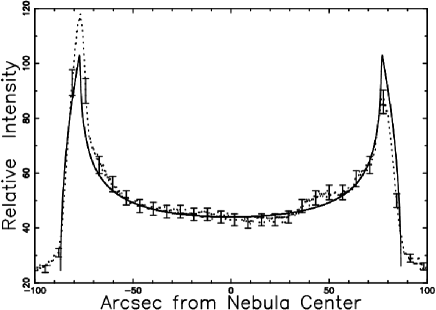
Figure 1: Cut of the relative intensity of A39 crossing the center in the east-west direction (dotted line with some error bar) and the rim model (full line) fully described in  Jacoby et al. (2001) , $\rm\chi^{2}$ = 0.505 when 5819 point are considered.

In presence of real data a merit function ,$\rm\chi^{2}$ , is introduced as

$$\chi^{2}=\frac{1}{N}\sum_{i=1}^{N}\bigl{[}\frac{y_{i}-y_{i,obs}}{\sigma_{i}}\bigr{]}^{2}\quad,$$ (4)

where $\rm N$ is the number of the data , $\rm y_{i}$ the theoretical ith point , $\rm y_{i,obs}$ the ith observed point and $\rm\sigma_{i}$ the error for the ith observed point here computed as $\rm\frac{y_{i}}{10}$.

2.2 The asymmetric PN

The Ring nebula , also known as M57 or NGC6720 , presents an elliptical shape characterized by a semi-major axis of $\rm 42^{\prime\prime}$, a semi-minor axis of $\rm 29.4^{\prime\prime}$ and ellipticity of 0.7, see Table I in Hiriart (2004). The distance of the Ring nebula is not very well known ; according to Harris et al. (1997) the distance is 705 $\rm pc$ . In physical units the two radii are

$$\rm\displaystyle R_{shell,minor}=0.1\Theta_{29.4}D_{705}~{}pc\quad~{}~{}~{}semi-minor~{}radius$$

$$\rm\displaystyle R_{shell,major}=0.14\Theta_{42}D_{705}~{}pc\quad~{}~{}~{}semi-major~{}radius\quad,$$ (5)

where $\rm\Theta_{29.4}$ is the angular minor radius in units of $\rm 29.4^{\prime\prime}$, $\rm\Theta_{42}$ is the angular major radius in units of $\rm 42^{\prime\prime}$ and $\rm D_{705}$ the distance in units of 705 $\rm pc$. The radial velocity structure in the Ring Nebula was derived from observations of the $\rm H_{2}$ (molecular Hydrogen)   v = 1- 0 S(1) emission line at 2.122 $\rm\mu m$ obtained by using a cooled Fabry- Perot etalon and a near-infrared imaging detector , see Hiriart (2004) . The velocity structure of the Ring Nebula covers the range $\rm[-30.3\leftrightarrow 48.8~{}\frac{km}{s}]$ .

2.3 The case of MyCn 18

MyCn 18 is a PN at a distance of 2.4 $\rm kpc$ and clearly shows an hourglass-shaped nebula, see Corradi & Schwarz (1993); Sahai et al. (1999). On referring to Table 1 in Dayal et al. (2000) we can fix the equatorial radius in $\rm 2.80\times 10^{16}~{}cm$ , or $\rm 0.09~{}pc$ , and the radius at $\rm 60^{\circ}$ from the equatorial plane $\rm 3.16\times 10^{17}~{}cm$ or $\rm 0.102~{}pc$ . The determination of the observed field of velocity of MyCn 18 varies from an overall value of 10 $\rm\frac{km}{s}$ as suggested by the expansion of $\rm[OIII]$ , see Sahai et al. (1999) , to a theoretical model by Dayal et al. (2000) in which the velocity is 9.6 $\rm\frac{km}{s}$ when the latitude is 0 ^∘ (equatorial plane) to 40.9 $\rm\frac{km}{s}$ when the latitude is 60 ^∘.

3 Law of motion

This Section presents two solutions for the law of motion that describe asymmetric expansion. The momentum conservation is then applied in cases where the density of the interstellar medium is not constant but regulated by exponential behavior.

3.1 Spherical Symmetry - Sedov solution

The momentum conservation is applied to a conical section of radius $\rm R$ with a solid angle $\rm\Delta\;\Omega$, in polar coordinates, see  McCray & Layzer (1987)

$$\frac{d}{dt}(\Delta MR)=\Delta F\,,$$ (6)

where

$$\Delta M=\int_{0}^{R}\rho(R,\theta,\phi)dV\,,$$ (7)

is the mass of swept–up interstellar medium in the solid angle $\rm\Delta\;\Omega$, $\rm\rho$ the density of the medium , $\rm P$ the interior pressure and the driving force:

$$\Delta\;F=PR^{2}\Delta\Omega\,.$$ (8)

After some algebra the Sedov solution is obtained, see Sedov (1959); McCray & Layzer (1987)

$$R(t)=\left({\frac{25}{4}}\,{\frac{{\it E}\,{t}^{2}}{\pi\,\rho}}\right)^{1/5}\quad,$$ (9)

where $\rm E$ is the energy injected in the process and $\rm t$ the time.

Another slightly different solution is formula (7.56) in Dyson & Williams (1997)

$$R(t)=\left({\frac{25}{3}}\,{\frac{{\it E}\,{t}^{2}}{\pi\,\rho}}\right)^{1/5}\quad,$$ (10)

where the difference is due to the adopted approximations.

Our astrophysical units are: time ($\rm t_{4}$), which is expressed in $\rm 10^{4}$ yr units; $\rm E_{42}$, the energy in $\rm 10^{42}$ erg; and $\rm n_{0}$ the number density expressed in particles $\rm\mathrm{cm}^{-3}$  (density $\rm\rho=n_{0}$m, where m=1.4$\rm m_{\mathrm{H}}$). With these units equation (9) becomes

$$R(t)\approx 0.198\left({\frac{{\it E_{42}}\,{t_{4}}^{2}}{n_{0}}}\right)^{1/5}~{}pc\quad.$$ (11)

The expansion velocity is

$$V(t)=\frac{2}{5}\frac{R(t)}{t}\quad,$$ (12)

which expressed in astrophysical units is

$$V(t)\approx 7.746\,{\frac{\sqrt[5]{{\it E_{42}}}}{\sqrt[5]{{\it n_{0}}}{{\it t_{4}}}^{3/5}}}~{}\frac{km}{s}\quad.$$ (13)

By inserting $\rm M_{\sun}$=0.605 and $\rm R_{pc}$=1 in formula (1) we obtain $\rm n\approx 6.28\frac{particles}{cm^{3}}$ . This value is higher than the value of number density of the ISM at the plane of the galaxy, $\rm n\approx 1\frac{particles}{cm^{3}}$ . Equations (11) and (13) represent a system of two equations in two unknowns : $\rm t_{4}$ and $\rm E_{42}$ . By inserting for example $\rm R=0.78~{}pc$ in equation (11) we find

$$t_{4}=77.15\,{\frac{1}{\sqrt{{\it E_{42}}}}}\quad,$$ (14)

and inserting $\rm V=35~{}km\;s^{-1}$ in equation (13) we obtain

$$0.3954\,\sqrt{{\it E_{42}}}=35\quad.$$ (15)

The previous equation is solved for $\rm E_{42}=7833.4$ that according to equation (14) means $\rm t_{4}$=.87173. These two parameters allows a rough evaluation of the mechanical luminosity $\rm L=\frac{E}{t}$ that turns out to be $\rm L\approx 2.847\;10^{34}ergs\;s^{-1}$. This value should be bigger than the observed luminosities in the various bands. As an example the X-ray luminosity of PNs , $\rm L_{X}$, in the wavelength band 5-28 Å  has a range $\rm[10^{30.9}\leftrightarrow 10^{31.2}ergs\;s^{-1}]$ , see Table 3 in Steffen et al. (2008).

Due to the fact that is difficult to compute the volume in an asymmetric expansion the Sedov solution is adopted only in this paragraph.

3.2 Spherical Symmetry - Momentum Conservation

The thin layer approximation assumes that all the swept-up gas accumulates infinitely in a thin shell just after the shock front. The conservation of the radial momentum requires that

$$\frac{4}{3}\pi R^{3}\rho\dot{R}=M_{0}\quad,$$ (16)

where $\rm R$ and $\rm\dot{R}$ are the radius and the velocity of the advancing shock , $\rm\rho$ the density of the ambient medium , $\rm M_{0}$ the momentum evaluated at $\rm t=t_{0}$ , $\rm R_{0}$ the initial radius and $\rm\dot{R_{0}}$ the initial velocity , see Dyson & Williams (1997); Padmanabhan (2001). The law of motion is

$$R=R_{0}\left(1+4\frac{\dot{R_{0}}}{R_{0}}(t-t_{0})\right)^{\frac{1}{4}}\quad.$$ (17)

and the velocity

$$\dot{R}=\dot{R_{0}}\left(1+4\frac{\dot{R_{0}}}{R_{0}}(t-t_{0})\right)^{-\frac{3}{4}}\quad.$$ (18)

From equation (17) we can extract $\rm\dot{R_{0}}$ and insert it in equation (18)

$$\dot{R}=\frac{1}{4(t-t_{0})}\frac{R^{4}-R_{0}^{4}}{R_{0}^{3}}\left(1+\frac{R^{4}-R_{0}^{4}}{R_{0}^{4}}\right)^{-\frac{3}{4}}\quad.$$ (19)

The astrophysical units are: $\rm t_{4}$ and $\rm t_{0,4}$ which are $\rm t$ and $\rm t_{0}$ expressed in $\rm 10^{4}$ yr units, $\rm R_{pc}$ and $\rm R_{0,pc}$ which are $\rm R$ and $\rm R_{0}$ expressed in $\rm pc$, $\rm\dot{R}_{kms}$ and $\rm\dot{R}_{0,kms}$ which are $\rm\dot{R}$ and $\rm\dot{R}_{0}$ expressed in $\rm\frac{km}{s}$. Therefore the previous formula becomes

$$\dot{R}_{kms}=24.49\frac{1}{(t_{4}-t_{0,4})}\frac{R_{pc}^{4}-R_{0,pc}^{4}}{R_{0,pc}^{3}}\left(1+\frac{R_{pc}^{4}-R_{0,pc}^{4}}{R_{0,pc}^{4}}\right)^{-\frac{3}{4}}\quad.$$ (20)

On introducing $\rm R_{0,pc}=0.1$ , $\rm R_{pc}=0.78$ , $\rm\dot{R}_{kms}=34.5\frac{km}{s}$ , the approximated age of A39 is found to be $\rm t_{4}-t_{0,4}=50$ and $\rm\dot{R}_{0,kms}=181.2$.

3.3 Asymmetry - Momentum Conservation

Given the Cartesian coordinate system $\rm(x,y,z)$ , the plane $\rm z=0$ will be called equatorial plane and in polar coordinates $\rm z=R\sin(\theta)$, where $\rm\theta$ is the polar angle and $\rm R$ the distance from the origin . The presence of a non homogeneous medium in which the expansion takes place can be modeled assuming an exponential behavior for the number of particles of the type

$$n(z)=n_{0}\exp{-\frac{z}{h}}\quad=n_{0}\exp{-\frac{R\times\sin(\theta)}{h}}\quad,$$ (21)

where $\rm R$ is the radius of the shell , $\rm n_{0}$ is the number of particles at $\rm R=R_{0}$ and $\rm h$ the scale. The 3D expansion will be characterized by the following properties

• Dependence of the momentary radius of the shell on the polar angle $\rm\theta$ that has a range $\rm[-90^{\circ}\leftrightarrow+90^{\circ}]$.

• Independence of the momentary radius of the shell from $\rm\phi$ , the azimuthal angle in the x-y plane, that has a range $\rm[0^{\circ}\leftrightarrow 360^{\circ}]$.

The mass swept, $\rm M$, along the solid angle $\rm\Delta\;\Omega$, between 0 and $\rm R$ is

$$M(R)=\frac{\Delta\;\Omega}{3}m_{H}n_{0}I_{m}(R)+\frac{4}{3}\pi R_{0}^{3}n_{0}m_{H}\quad,$$ (22)

where

$$I_{m}(R)=\int_{R_{0}}^{R}r^{2}\exp{-\frac{r\sin(\theta)}{h}}dr\quad,$$ (23)

where $\rm R_{0}$ is the initial radius and $\rm m_{H}$ the mass of the hydrogen . The integral is

$$\rm\displaystyle I_{m}(R)=\frac{h\left(2\,{h}^{2}+2\,R_{0}h\sin\left(\theta\right)+{R_{0}}^{2}\left(\sin\left(\theta\right)\right)^{2}\right){{\rm e}^{-{\frac{R_{0}\sin\left(\theta\right)}{h}}}}}{\left(\sin\left(\theta\right)\right)^{3}}$$

$$\rm\displaystyle-\frac{h\left(2\,{h}^{2}+2\,Rh\sin\left(\theta\right)+{R}^{2}\left(\sin\left(\theta\right)\right)^{2}\right){{\rm e}^{-{\frac{R\sin\left(\theta\right)}{h}}}}}{\left(\sin\left(\theta\right)\right)^{3}}\quad.$$ (24)

The conservation of the momentum gives

$$M(R)\dot{R}=M(R_{0})\dot{R_{0}}\quad,$$ (25)

where $\rm\dot{R}$ is the velocity at $\rm R$ and $\rm\dot{R_{0}}$ the initial velocity at $\rm R=R_{0}$.

In this differential equation of the first order in $\rm R$ the variable can be separated and the integration term by term gives

$$\int_{R_{0}}^{R}M(r)dr=M(R_{0})\dot{R_{0}}\times(t-t_{0})\quad,$$ (26)

where $\rm t$ is the time and $\rm t_{0}$ the time at $\rm R_{0}$. The resulting non linear equation $\rm{\mathcal{F}}_{NL}$ expressed in astrophysical units is

$$\rm\displaystyle{\mathcal{F}}_{NL}=-6\,{{\rm e}^{-\,{\frac{{\it R_{0,pc}}\,\sin\left(\theta\right)}{{\it h_{pc}}}}}}{{\it h_{pc}}}^{4}-\,{\it h_{pc}}\,{{\rm e}^{-\,{\frac{{\it R_{0,pc}}\,\sin\left(\theta\right)}{{\it h_{pc}}}}}}\left(\sin\left(\theta\right)\right)^{3}{{\it R_{0,pc}}}^{3}$$

$$\rm\displaystyle-6\,{{\it h_{pc}}}^{3}{{\rm e}^{-\,{\frac{{\it R_{0,pc}}\,\sin\left(\theta\right)}{{\it h_{pc}}}}}}\sin\left(\theta\right){\it R_{0,pc}}-3\,{{\it h_{pc}}}^{2}{{\rm e}^{-\,{\frac{{\it R_{0,pc}}\,\sin\left(\theta\right)}{{\it h_{pc}}}}}}\left(\sin\left(\theta\right)\right)^{2}{{\it R_{0,pc}}}^{2}$$

$$\rm\displaystyle-\,{{\it R_{0,pc}}}^{4}\left(\sin\left(\theta\right)\right)^{4}+6\,{{\rm e}^{-\,{\frac{{\it R_{pc}}\,\sin\left(\theta\right)}{{\it h_{pc}}}}}}{{\it h_{pc}}}^{4}+4\,{{\rm e}^{-\,{\frac{{\it R_{pc}}\,\sin\left(\theta\right)}{{\it h_{pc}}}}}}{{\it h_{pc}}}^{3}{\it R_{pc}}\,\sin\left(\theta\right)$$

$$\rm\displaystyle+{{\rm e}^{-\,{\frac{{\it R_{pc}}\,\sin\left(\theta\right)}{{\it h_{pc}}}}}}{{\it h_{pc}}}^{2}{{\it R_{pc}}}^{2}\left(\sin\left(\theta\right)\right)^{2}$$

$$\rm\displaystyle+2\,{{\rm e}^{-\,{\frac{{\it R_{0,pc}}\,\sin\left(\theta\right)}{{\it h_{pc}}}}}}{{\it h_{pc}}}^{3}{\it R_{pc}}\,\sin\left(\theta\right)+2\,{{\rm e}^{-\,{\frac{{\it R_{0,pc}}\,\sin\left(\theta\right)}{{\it h_{pc}}}}}}{{\it h_{pc}}}^{2}{\it R_{pc}}\,\left(\sin\left(\theta\right)\right)^{2}{\it R_{0,pc}}$$

$$\rm\displaystyle+{{\rm e}^{-\,{\frac{{\it R_{0,pc}}\,\sin\left(\theta\right)}{{\it h_{pc}}}}}}{\it h_{pc}}\,{\it R_{pc}}\,\left(\sin\left(\theta\right)\right)^{3}{{\it R_{0,pc}}}^{2}$$

$$\rm\displaystyle+\left(\sin\left(\theta\right)\right)^{4}{{\it R_{0,pc}}}^{3}{\it R_{pc}}-0.01\left(\sin\left(\theta\right)\right)^{4}{{\it R_{0,pc}}}^{3}{\dot{R}_{0,kms}}\,\left(t_{4}-t_{0,4}\right)=0\quad,$$ (27)

where $\rm t_{4}$ and $\rm t_{0,4}$ are $\rm t$ and $\rm t_{0}$ expressed in $\rm 10^{4}$ yr units, $\rm R_{pc}$ and $\rm R_{0,pc}$ are $\rm R$ and $\rm R_{0}$ expressed in $\rm pc$, $\rm\dot{R}_{kms}$ and $\rm\dot{R}_{0,kms}$ are $\rm\dot{R}$ and $\rm\dot{R}_{0}$ expressed in $\rm\frac{km}{s}$, $\rm\theta$ is expressed in radians and $\rm h_{pc}$ is the the scale , $\rm h$ , expressed in $\rm pc$. It is not possible to find $\rm R_{pc}$ analytically and a numerical method should be implemented. In our case in order to find the root of $\rm{\mathcal{F}}_{NL}$, the FORTRAN SUBROUTINE ZRIDDR from Press et al. (1992) has been used.

The unknown parameter $\rm t_{4}-t_{0,4}$ can be found from different runs of the code once $\rm R_{0,pc}$ is fixed as $\rm\approx$ 1/10 of the observed equatorial radius , $\rm\dot{R}_{0,kms}$ is 200 or less and $\rm h_{pc}\approx 2\times R_{0,pc}$.

From a practical point of view, $\rm\epsilon$ , the percentage of reliability of our code can also be introduced,

$$\epsilon=(1-\frac{|(R_{\mathrm{pc,obs}}-R_{pc,\mathrm{num}})|}{R_{pc,\mathrm{obs}}})\cdot 100\,,$$ (28)

where $\rm R_{pc,\mathrm{obs}}$ is the radius as given by the astronomical observations in parsec , and $\rm R_{pc,\mathrm{num}}$ the radius obtained from our simulation in parsec.

In order to test the simulation over different angles, an observational percentage of reliability ,$\rm\epsilon_{\mathrm{obs}}$, is introduced which uses both the size and the shape,

$$\epsilon_{\mathrm{obs}}=100(1-\frac{\sum_{j}|R_{pc,\mathrm{obs}}-R_{pc,\mathrm{num}}|_{j}}{\sum_{j}{R_{pc,\mathrm{obs}}}_{,j}}),$$ (29)

where the index $\rm j$ varies from 1 to the number of available observations.

3.3.1 Simulation of the Ring nebula

A typical set of parameters that allows us to simulate the Ring nebula is reported in Table 1.

Table 1: Data of the simulation of the Ring nebula

$$\rm\rm\begin{array}[]{cc}\hline\cr\vskip 3.0pt plus 1.0pt minus 1.0pt\cr\mbox{Initial ~{}expansion~{}velocity~{},$\rm{\dot{R}}_{{0,kms}}$ }&200\\ \mbox{Age~{}($\rm t_{4}-t_{0,4}$) }&0.12\\ \mbox{Initial~{}radius~{} $\rm R_{0,pc}$ }&0.035\\ \mbox{scaling~{} $\rm h_{pc}$ }&\mbox{$\rm 2\times R_{0,pc}$}\\ \vskip 3.0pt plus 1.0pt minus 1.0pt\cr\hline\cr\end{array}$$

The complex 3D behavior of the advancing Ring nebula is reported in Figure 2 and Figure 3 reports the asymmetric expansion in a section crossing the center. In order to better visualize the asymmetries Figure 4 and Figure 5 report the radius and the velocity as a function of the position angle $\rm\theta$. The combined effect of spatial asymmetry and field of velocity are reported in Figure 6.

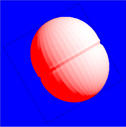
Figure 2: Continuous three-dimensional surface of the Ring nebula : the three Eulerian angles characterizing the point of view are $\rm\Phi$=180 ^∘, $\rm\Theta$=90 ^∘ and $\rm\Psi$=-30 ^∘. Physical parameters as in Table 1.

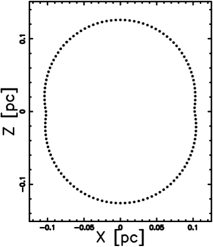
Figure 3: Section of the Ring nebula on the x-z plane. The horizontal and vertical axis are in $\rm pc$. Physical parameters as in Table 1.

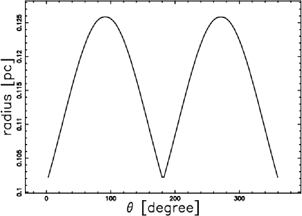
Figure 4: Radius in $\rm pc$ of the Ring nebula as a function of the position angle in degrees. Physical parameters as in Table 1.

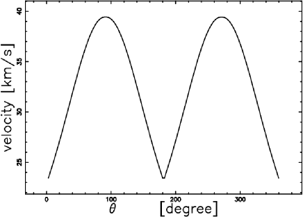
Figure 5: Velocity in $\rm\frac{km}{s}$ of the Ring nebula as a function of the position angle in degrees. Physical parameters as in Table 1.

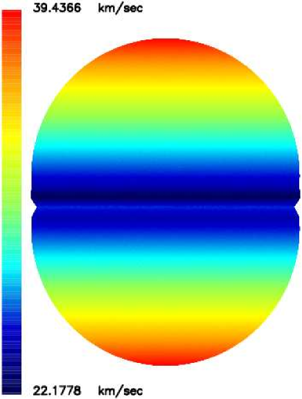
Figure 6: Map of the expansion velocity in $\rm\frac{km}{s}$ relative to the simulation of the Ring nebula when 300000 random points are selected on the surface. Physical parameters as in Table 1.

The efficiency of our code in reproducing the observed radii as given by formula (28 ) and the efficiency when the age is five time greater are reported in Table 2.

An analogous formula allows us to compute the efficiency in the computation of the maximum velocity , see Table 3.

Table 2: Reliability of the radii of the Ring nebula.

$$\rm\rm\begin{array}[]{lccc}\hline\cr\vskip 3.0pt plus 1.0pt minus 1.0pt\cr{}{}{}{}&R_{\mathrm{up}}(\mathrm{pc})~{}polar~{}direction&R_{\mathrm{eq}}(\mathrm{pc})~{}equatorial~{}plane\\ \vskip 3.0pt plus 1.0pt minus 1.0pt\cr\hline\cr\vskip 3.0pt plus 1.0pt minus 1.0pt\cr R_{\mathrm{obs}}&0.14&0.1\\ R_{\mathrm{num}}(\mbox{our~{}code})&0.125&0.102\\ \mbox{$\rm\epsilon$}(\%)&89&97\\ \mbox{$\rm\epsilon$}~{}(\%)~{}for~{}a~{}time~{}5~{}times~{}greater&27&41\\ \vskip 3.0pt plus 1.0pt minus 1.0pt\cr\hline\cr\end{array}$$

Table 3: Reliability of the velocity of the Ring nebula

$$\rm\rm\begin{array}[]{lc}\hline\cr\vskip 3.0pt plus 1.0pt minus 1.0pt\cr{}{}{}{}&V({\frac{km}{s}})~{}maximum~{}velocity\\ \vskip 3.0pt plus 1.0pt minus 1.0pt\cr\hline\cr\vskip 3.0pt plus 1.0pt minus 1.0pt\cr V_{\mathrm{obs}}&48.79\\ V_{\mathrm{num}}&39.43\\ \mbox{$\rm\epsilon$}(\%)&80.81\\ \mbox{$\rm\epsilon$}(\%)~{}(\%)~{}for~{}a~{}time~{}5~{}times~{}greater&35.67\\ \vskip 3.0pt plus 1.0pt minus 1.0pt\cr\hline\cr\end{array}$$

3.3.2 Simulation of MyCn 18

A typical set of parameters that allows us to simulate MyCn 18 is reported in Table 4.

Table 4: Data of the simulation of MyCn 18

$$\rm\rm\begin{array}[]{cc}\hline\cr\vskip 3.0pt plus 1.0pt minus 1.0pt\cr\mbox{Initial ~{}expansion~{}velocity~{},$\rm{\dot{R}}_{{0,kms}}$ [km~{}s$\rm{}^{-1}$}]&200\\ \mbox{Age~{}($\rm t_{4}-t_{0,4}$) [10$\rm{}^{4}$~{}yr]}&0.2\\ \mbox{Initial~{}radius~{} $\rm R_{0,pc}$ ~{}[pc] }&0.001\\ \mbox{scaling~{} h [pc] }&\mbox{$\rm 1.0\times R_{0}$}\\ \vskip 3.0pt plus 1.0pt minus 1.0pt\cr\hline\cr\end{array}$$

The bipolar behavior of the advancing MyCn 18 is reported in Figure 7 and Figure 8 reports the expansion in a section crossing the center. It is interesting to point out the similarities between our Figure 8 of MyCn 18 and Figure 1 in Morisset & Stasinska (2008) which define the parameters $\rm a$ and $\rm h$ of the Atlas of synthetic line profiles. In order to better visualize the two lobes Figure 9 reports the radius as a function of the position angle $\rm\theta$.

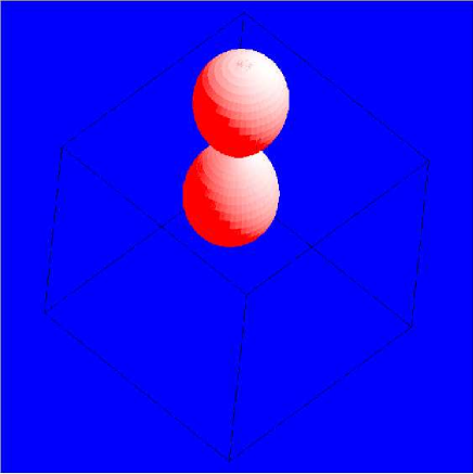
Figure 7: Continuous three-dimensional surface of MyCn 18 : the three Eulerian angles characterizing the point of view are $\rm\Phi$=130 ^∘, $\rm\Theta$=40 ^∘ and $\rm\Psi$=5 ^∘. Physical parameters as in Table 4.

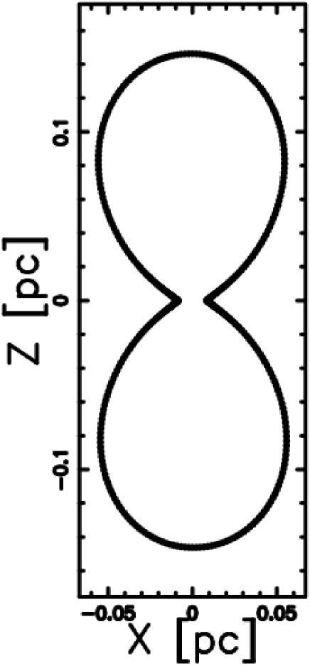
Figure 8: Section of MyCn 18 on the x-z plane. Physical parameters as in Table 4.

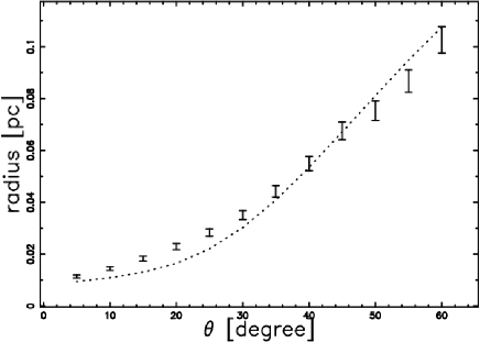
Figure 9: Radius in pc of MyCn 18 as a function of latitude from $\rm 0^{\circ}$ to $\rm 60^{\circ}$ ( dotted line) when the physical parameters are those of Table 4. The points with error bar (1/10 of the value) represent the data of Table 1 in Dayal et al. 2000.

The combined effect of spatial asymmetry and field of velocity are reported in Figure 10.

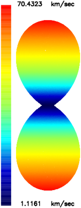
Figure 10: Map of the expansion velocity in $\rm\frac{km}{s}$ relative to the simulation of MyCn 18 when 300000 random points are selected on the surface. Physical parameters as in Table 4.

The efficiency of our code in reproducing the spatial shape over 12 directions of MyCn 18 as given by formula (29 ) is reported in Table 5. This Table also reports the efficiency in simulating the shape of the velocity.

Table 5: Reliability of the spatial and velocity shape of MyCn 18.

$$\rm\rm\begin{array}[]{lcc}\hline\cr\vskip 3.0pt plus 1.0pt minus 1.0pt\cr{}{}{}&radius&velocity\\ \mbox{$\rm\epsilon_{obs}$}(\%)&90.66&57.68\\ \vskip 3.0pt plus 1.0pt minus 1.0pt\cr\hline\cr\end{array}$$

Figure   11 reports our results as well those of Table 1 in Dayal et al. (2000).

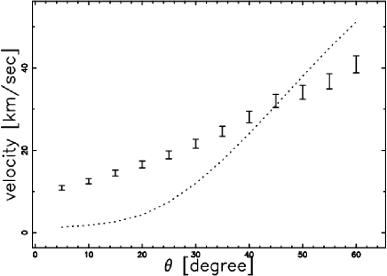
Figure 11: Velocity in $\rm\frac{km}{s}$ of MyCn 18 as a function of the latitude in degrees when the physical parameters are those of Table 4, dotted line. The points with error bar (1/10 of the value) represent the data of Table 1 in Dayal et al. 2000.

4 Diffusion

The mathematical diffusion allows us to follow the number density of particles from high values (injection) to low values (absorption). We recall that the number density is expressed in $\rm\frac{particles}{unit~{}volume}$ and the symbol $\rm C$ is used in the mathematical diffusion and the symbol $\rm n$ in an astrophysical context. The density $\rm\rho$ is obtained by multiplying $\rm n$ by the mass of hydrogen , $\rm m_{H}$ , and by a multiplicative factor , $\rm f$, which varies from 1.27 in Kim et al. (2000) to 1.4 in McCray & Layzer (1987)

$$\rho=fm_{H}n\quad.$$ (30)

The physical process that allows the particles to diffuse is hidden in the mathematical diffusion. In our case the physical process can be the random walk with a time step equal to the Larmor gyroradius. In the Monte Carlo diffusion the step-length of the random walk is generally taken as a fraction of the side of the considered box. Both mathematical diffusion and Monte Carlo diffusion use the concept of absorbing-boundary which is the spatial coordinate where the diffusion path terminates.

In the following, 3D mathematical diffusion from a sphere and 1D mathematical as well Monte Carlo diffusion in presence of drift are considered.

4.1 3D diffusion from a spherical source

Once the number density , $\rm C$, and the diffusion coefficient ,$\rm D$, are introduced , Fick’ s first equation changes expression on the basis of the adopted environment , see for example equation (2.5) in Berg (1993). In three dimensions it is

$$\frac{\partial C}{\partial t}=D\nabla^{2}C\quad,$$ (31)

where $\rm t$ is the time and $\rm\nabla^{2}$ is the Laplacian differential operator.

In presence of the steady state condition:

$$D\nabla^{2}C=0\quad.$$ (32)

The number density rises from 0 at r=a to a maximum value $\rm C_{m}$ at r=b and then falls again to 0 at r=c . The solution to equation (32) is

$$C(r)=A+\frac{B}{r}\quad,$$ (33)

where $\rm A$ and $\rm B$ are determined by the boundary conditions ,

$$C_{ab}(r)=C_{{m}}\left(1-{\frac{a}{r}}\right)\left(1-{\frac{a}{b}}\right)^{-1}\quad a\leq r\leq b\quad,$$ (34)

and

$$C_{bc}(r)=C_{{m}}\left({\frac{c}{r}}-1\right)\left({\frac{c}{b}}-1\right)^{-1}\quad b\leq r\leq c\quad.$$ (35)

These solutions can be found in Berg (1993) or in Crank (1979) .

4.2 1D diffusion with drift, mathematical diffusion

In one dimension and in the presence of a drift velocity ,$\rm u$, along the radial direction the diffusion is governed by Fick’s second equation , see equation (4.5) in Berg (1993) ,

$$\frac{\partial C}{\partial t}=D\frac{\partial^{2}C}{\partial r^{2}}-{\vec{u}}\frac{\partial C}{\partial r}\quad,$$ (36)

where $\rm{\vec{u}}$ can take two directions. The number density rises from 0 at r=a to a maximum value $\rm C_{m}$ at r=b and then falls again to 0 at r=c . The general solution to equation (36) in presence of a steady state is

$$C(r)=A+Be^{{\frac{\vec{u}}{D}}r}\quad.$$ (37)

We now assume that u and r do not have the same direction and therefore u is negative ; the solution is

$$C(r)=A+Be^{-{\frac{u}{D}}r}\quad,$$ (38)

and now the velocity $\rm u$ is a scalar.

The boundary-conditions give

$$C_{a,b,drift}(r)=C_{m}\frac{e^{-\frac{u}{D}a}-e^{-\frac{u}{D}r}}{e^{-\frac{u}{D}a}-e^{-\frac{u}{D}b}}\quad a\leq r\leq b~{}\quad downstream~{}side\quad,$$ (39)

and

$$C_{b,c,drift}(r)=C_{m}\frac{e^{-\frac{u}{D}c}-e^{-\frac{u}{D}r}}{e^{-\frac{u}{D}c}-e^{-\frac{u}{D}b}}\quad b\leq r\leq c~{}\quad upstream~{}side\quad.$$ (40)

A typical plot of the number density for different values of the diffusion coefficient is reported in Figure 12.

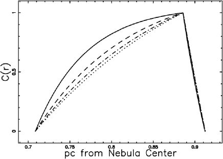
Figure 12: Number density of A39 as a function of the distance in pc from the injection when $\rm u=1$ , $\rm C_{m}=1$, $\rm a=69.6~{}arcsec$, $\rm b=87~{}arcsec$ , $\rm c=89.6~{}arcsec$ and $\rm D=2$ (full line ), $\rm D=7$ (dashed ), $\rm D=12$ (dot-dash-dot-dash) and $\rm D=17$ (dotted ). The conversion from $\rm arcsec$ to $\rm pc$ is done assuming a distance of 2100 $\rm pc$ for A39.

4.3 1D diffusion with drift, random walk

Given a 1D segment of length $\rm side$ we can implement the random walk with step-length $\rm\lambda$ by introducing the numerical parameter $\rm NDIM=\frac{side}{\lambda}$ . We now report the adopted rules when the injection is in the middle of the grid :

1. The first of the $\rm NPART$ particles is chosen.

2. The random walk of a particle starts in the middle of the grid. The probabilities of having one step are $\rm p_{1}$ in the negative direction (downstream) ,$\rm p_{1}=\frac{1}{2}-\mu\times\frac{1}{2}$, and $\rm p_{2}$ in the positive direction (upstream) , $\rm p_{2}=\frac{1}{2}+\mu\times\frac{1}{2}$, where $\rm\mu$ is a parameter that characterizes the asymmetry ($\rm 0\leq\mu\leq 1$).

3. When the particle reaches one of the two absorbing points , the motion starts another time from (ii) with a different diffusing pattern.

4. The number of visits is recorded on $\rm{\mathcal{M}}$ , a one–dimensional grid.

5. The random walk terminates when all the $\rm NPART$ particles are processed.

6. For the sake of normalization the one–dimensional visitation or number density grid $\rm{\mathcal{M}}$ is divided by $\rm NPART$.

There is a systematic change of the average particle position along the $\rm x$-direction:

$$\langle dx\rangle=\mu~{}\lambda\quad,$$ (41)

for each time step. If the time step is $\rm dt=\frac{\lambda}{v_{tr}}$ where $\rm{v_{tr}}$ is the transport velocity, the asymmetry ,$\rm\mu$ , that characterizes the random walk is

$$\mu=\frac{u}{v_{tr}}\quad.$$ (42)

Figure 13 reports $\rm{\mathcal{M}}(x)$, the number of visits generated by the Monte Carlo simulation as well as the mathematical solution represented by formulas (39) and (40).

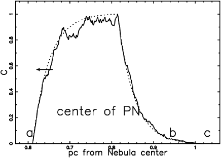
Figure 13: Number density in A39 of the 1D asymmetric random walk (full line), NDIM=401 ,NPART=200 ,$\rm side=40~{}arcsec$ , $\rm\lambda=0.1~{}arcsec$ and $\rm\mu$ =- 0.013. For astrophysical purposes $\rm\mu$ is negative. The theoretical number density as represented by formulas (39) and (40) is reported when $\rm u=1$ , $\rm C_{m}=1$, $\rm a=60~{}arcsec$, $\rm b=80~{}arcsec$ , $\rm c=100~{}arcsec$ and $\rm D=3.84$ (dotted line ). The conversion from $\rm arcsec$ to $\rm pc$ is done assuming a distance of 2100 $\rm pc$ for A39.

The solutions of the mathematical diffusion equations (39) and (40) can be rewritten at the light of the random walk and are

$$C_{a,b,MC}(r)=C_{m}\frac{e^{-\frac{2\mu}{\lambda}a}-e^{-\frac{2\mu}{\lambda}r}}{e^{-\frac{2\mu}{\lambda}a}-e^{-\frac{2\mu}{\lambda}b}}\quad a\leq r\leq b~{}\quad downstream~{}side\quad,$$ (43)

and

$$C_{b,c,MC}(r)=C_{m}\frac{e^{-\frac{2\mu}{\lambda}c}-e^{-\frac{2\mu}{\lambda}r}}{e^{-\frac{2\mu}{\lambda}c}-e^{-\frac{2\mu}{\lambda}b}}\quad b\leq r\leq c~{}\quad upstream~{}side\quad.$$ (44)

5 The Image of the PN

The image of a PN can be easily modeled once an analytical or numerical law for the intensity of emission as a function of the radial distance from the center is given. Simple analytical results for the radial intensity can be deduced in the rim model when the length of the layer and the number density are constants and in the spherical model when the number density is constant.

The integration of the solutions to the mathematical diffusion along the line of sight allows us to deduce analytical formulas in the spherical case. The complexity of the intensity in the aspherical case can be attached only from a numerical point of view.

5.1 Radiative transfer equation

The transfer equation in the presence of emission only , see for example Rybicki & Lightman (1985) or Hjellming (1988) , is

$$\frac{dI_{\nu}}{ds}=-k_{\nu}\zeta I_{\nu}+j_{\nu}\zeta\quad,$$ (45)

where $\rm I_{\nu}$ is the specific intensity , $\rm s$ is the line of sight , $\rm j_{\nu}$ the emission coefficient, $\rm k_{\nu}$ a mass absorption coefficient, $\rm\zeta$ the mass density at position s and the index $\rm\nu$ denotes the interested frequency of emission. The solution to equation (45) is

$$I_{\nu}(\tau_{\nu})=\frac{j_{\nu}}{k_{\nu}}(1-e^{-\tau_{\nu}(s)})\quad,$$ (46)

where $\rm\tau_{\nu}$ is the optical depth at frequency $\rm\nu$

$$d\tau_{\nu}=k_{\nu}\zeta ds\quad.$$ (47)

We now continue analyzing the case of an optically thin layer in which $\rm\tau_{\nu}$ is very small ( or $\rm k_{\nu}$ very small ) and the density $\rm\zeta$ is substituted with our number density C(s) of particles. Two cases are taken into account : the emissivity is proportional to the number density and the emissivity is proportional to the square of the number density . In the linear case

$$j_{\nu}\zeta=KC(s)\quad,$$ (48)

where $\rm K$ is a constant function. This can be the case of synchrotron radiation from an ensemble of particles , see formula (1.175 ) in Lang (1999) . This non thermal radiation continuum emission was detected in a PN associated with a very long-period OH/IR variable star (V1018 Sco), see Cohen et al. (2006).

In the quadratic case

$$j_{\nu}\zeta=K_{2}C(s)^{2}\quad,$$ (49)

where $\rm K_{2}$ is a constant function. This is true for

• Free-free radiation from a thermal plasma, see formula (1.219) in Lang (1999) . This radiation process was adopted by González et al. (2006) in the little Homunculus.

• Thermal bremsstrahlung and recombination radiation , see formula (1.237) in Lang (1999) . This radiation process was adopted in PNs by Blagrave et al. (2006); Schwarz & Monteiro (2006); Gruenwald & Aleman (2007).

The intensity is now

$$I_{\nu}(s)=K\int_{s_{0}}^{s}C(s\prime)ds\prime\quad\mbox{optically thin layer}\quad linear~{}case\quad,$$ (50)

or

$$I_{\nu}(s)=K_{2}\int_{s_{0}}^{s}C(s\prime)^{2}ds\prime\quad\mbox{optically thin layer}\quad quadratic~{}case\quad.$$ (51)

In the Monte Carlo experiments the number density is memorized on the grid $\rm{\mathcal{M}}$ and the intensity is

$${\it I}\/(i,j)=\sum_{k}\triangle\,s\times{\mathcal{M}}(i,j,k)\quad\mbox{optically thin layer}\quad linear~{}case\quad,$$ (52)

or

$${\it I}\/(i,j)=\sum_{k}\triangle\,s\times{\mathcal{M}}(i,j,k)^{2}\quad\mbox{optically thin layer}\quad quadratic~{}case\quad,$$ (53)

where $\rm\triangle$s is the spatial interval between the various values and the sum is performed over the interval of existence of the index $\rm k$. The theoretical intensity is then obtained by integrating the intensity at a given frequency over the solid angle of the source.

5.2 3D Constant Number density in a rim model

We assume that the number density $\rm C$ is constant and in particular rises from 0 at $\rm r=a$ to a maximum value $\rm C_{m}$ , remains constant up to $\rm r=b$ and then falls again to 0. This geometrical description is reported in Figure 14.

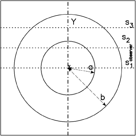
Figure 14: The two circles (section of spheres) which include the region with constant density are represented through a full line. The observer is situated along the x direction, and three lines of sight are indicated.

The length of sight , when the observer is situated at the infinity of the $\rm x$-axis , is the locus parallel to the $\rm x$-axis which crosses the position $\rm y$ in a Cartesian $\rm x-y$ plane and terminates at the external circle of radius $\rm b$. The locus length is

$$\rm\displaystyle l_{0a}=2\times(\sqrt{b^{2}-y^{2}}-\sqrt{a^{2}-y^{2}})\quad;0\leq y<a$$

$$\rm\displaystyle l_{ab}=2\times(\sqrt{b^{2}-y^{2}})\quad;a\leq y<b\quad.$$ (54)

When the number density $\rm C_{m}$ is constant between two spheres of radius $\rm a$ and $\rm b$ the intensity of radiation is

$$\rm\displaystyle I_{0a}=C_{m}\times 2\times(\sqrt{b^{2}-y^{2}}-\sqrt{a^{2}-y^{2}})\quad;0\leq y<a$$

$$\rm\displaystyle I_{ab}=C_{m}\times 2\times(\sqrt{b^{2}-y^{2}})\quad;a\leq y<b\quad.$$ (55)

The comparison of observed data of A39 and the theoretical intensity is reported in Figure 15 when data from Table 6 are used.

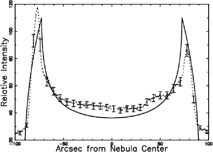
Figure 15: Cut of the mathematical intensity $\rm{\it I}$ of the rim model ( equation (55)) crossing the center (full line ) of A39 and real data (dotted line with some error bar ) . The number of data is 801 and for this model $\rm\chi^{2}$ = 1.487 against $\rm\chi^{2}$ = 0.862 of the rim model fully described in  Jacoby et al. (2001).

The ratio between the theoretical intensity at the maximum , $\rm(y=b)$ , and at the minimum , ($\rm y=0$) , is given by

$$\frac{I(y=b)}{I(y=0)}=\frac{\sqrt{b^{2}-a^{2}}}{b-a}\quad.$$ (56)

Table 6: Simulation of A39 with the rim model

$$\rm\rm\begin{array}[]{llc}\hline\cr\hline\cr\vskip 3.0pt plus 1.0pt minus 1.0pt\cr symbol&meaning&value\\ \vskip 3.0pt plus 1.0pt minus 1.0pt\cr\hline\cr\vskip 3.0pt plus 1.0pt minus 1.0pt\cr a&radius~{}of~{}the~{}internal~{}sphere&72.5^{\prime\prime}\\ \vskip 3.0pt plus 1.0pt minus 1.0pt\cr b&radius~{}of~{}the~{}external~{}sphere&90.18^{\prime\prime}\\ \vskip 3.0pt plus 1.0pt minus 1.0pt\cr R_{shell}&observed~{}radius~{}of~{}the~{}shell&77^{\prime\prime}\\ \vskip 3.0pt plus 1.0pt minus 1.0pt\cr\delta\,r_{shell,t}&theoretical~{}thickness~{}of~{}the~{}shell&17.6^{\prime\prime}\\ \vskip 3.0pt plus 1.0pt minus 1.0pt\cr\delta\,r_{shell}&observed~{}thickness~{}of~{}the~{}shell&10.1^{\prime\prime}\\ \vskip 3.0pt plus 1.0pt minus 1.0pt\cr\frac{I_{limb}}{I_{center}}&ratio~{}of~{}observed~{}intensities&(1.88-2.62)\\ \vskip 3.0pt plus 1.0pt minus 1.0pt\cr\frac{I_{max}}{I(y=0)}&ratio~{}of~{}theoretical~{}intensities&3.03\\ \vskip 3.0pt plus 1.0pt minus 1.0pt\cr\hline\cr\hline\cr\end{array}$$

5.3 3D Constant Number density in a spherical model

We assume that the number density $\rm C$ is constant in a sphere of radius $\rm a$ and then falls to 0.

The length of sight , when the observer is situated at the infinity of the $\rm x$-axis , is the locus parallel to the $\rm x$-axis which crosses the position $\rm y$ in a Cartesian $\rm x-y$ plane and terminates at the external circle of radius $\rm a$. The locus length is

$$\rm\displaystyle l_{ab}=2\times(\sqrt{a^{2}-y^{2}})\quad;0\leq y<a\quad.$$ (57)

When the number density $\rm C_{m}$ is constant in the sphere of radius $\rm a$ the intensity of radiation is

$$\rm\displaystyle I_{0a}=C_{m}\times 2\times(\sqrt{a^{2}-y^{2}})\quad;0\leq y<a\quad.$$ (58)

5.4 3D diffusion from a sphere

Figure 16 shows a spherical shell source of radius $\rm b$ between a spherical absorber of radius $\rm a$ and a spherical absorber of radius $\rm c$.

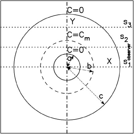
Figure 16: The spherical source inserted in the great box is represented through a dashed line, and the two absorbing boundaries with a full line. The observer is situated along the x direction, and three lines of sight are indicated. Adapted from Figure 3.1 by Berg (1993) .

The number density rises from 0 at r=a to a maximum value $\rm C_{m}$ at r=b and then falls again to 0 at r=c .

The numbers density to be used are formulas (34) and (35) once $\rm r=\sqrt{x^{2}+y^{2}}$ is imposed ; these two numbers density are inserted in formula (49) which represents the transfer equation with a quadratic dependence on the number density. An analogous case was solved in Zaninetti (2007) by adopting a linear dependence on the number density . The geometry of the phenomena fixes three different zones ($\rm 0-a,a-b,b-c$) in the variable $\rm y$, ; the first piece , $\rm I^{I}(y)$ , is

$$\rm\displaystyle I^{I}(y)=\int_{\sqrt{a^{2}-y^{2}}}^{\sqrt{b^{2}-y^{2}}}2C_{ab}^{2}dx+\int_{\sqrt{b^{2}-y^{2}}}^{\sqrt{c^{2}-y^{2}}}2C_{bc}^{2}dx$$

$$\rm\displaystyle~{}=-2\frac{{\it C_{m}}^{2}{b}^{2}}{y({b}^{2}-2\,ba+{a}^{2})({c}^{2}-2\,cb+{b}^{2})}\bigl{[}-2\,{a}^{2}\arctan({\frac{\sqrt{{a}^{2}-{y}^{2}}}{y}})cb-2\,\sqrt{{a}^{2}-{y}^{2}}ycb$$

$$\rm\displaystyle-2\,ay\ln(\sqrt{{a}^{2}-{y}^{2}}+a){b}^{2}+2\,{a}^{2}\arctan({\frac{\sqrt{{b}^{2}-{y}^{2}}}{y}})cb$$

$$\rm\displaystyle+2\,y\sqrt{{b}^{2}-{y}^{2}}cb+2\,a\ln(\sqrt{{b}^{2}-{y}^{2}}+b)y{b}^{2}+2\,a\ln(\sqrt{{b}^{2}-{y}^{2}}+b)y{c}^{2}$$

$$\rm\displaystyle-2\,cy\ln(\sqrt{{b}^{2}-{y}^{2}}+b){b}^{2}-2\,{c}^{2}\arctan({\frac{\sqrt{{b}^{2}-{y}^{2}}}{y}})ba-2\,y\sqrt{{b}^{2}-{y}^{2}}ba-$$

$$\rm\displaystyle 2\,cy\ln(\sqrt{{b}^{2}-{y}^{2}}+b){a}^{2}+2\,c\ln(\sqrt{{c}^{2}-{y}^{2}}+c)y{b}^{2}$$

$$\rm\displaystyle+2\,c\ln(\sqrt{{c}^{2}-{y}^{2}}+c)y{a}^{2}+2\,\sqrt{{c}^{2}-{y}^{2}}yba+2\,{c}^{2}\arctan({\frac{\sqrt{{c}^{2}-{y}^{2}}}{y}})ba$$

$$\rm\displaystyle-2\,ay\ln(\sqrt{{a}^{2}-{y}^{2}}+a){c}^{2}+\sqrt{{a}^{2}-{y}^{2}}y{c}^{2}$$

$$\rm\displaystyle-4\,c\ln(\sqrt{{c}^{2}-{y}^{2}}+c)yba+4\,ay\ln(\sqrt{{a}^{2}-{y}^{2}}+a)cb$$

$$\rm\displaystyle-\sqrt{{c}^{2}-{y}^{2}}y{a}^{2}+{a}^{2}\arctan({\frac{\sqrt{{a}^{2}-{y}^{2}}}{y}}){b}^{2}-y\sqrt{{b}^{2}-{y}^{2}}{c}^{2}-{c}^{2}\arctan({\frac{\sqrt{{c}^{2}-{y}^{2}}}{y}}){a}^{2}$$

$$\rm\displaystyle-\sqrt{{c}^{2}-{y}^{2}}y{b}^{2}+y\sqrt{{b}^{2}-{y}^{2}}{a}^{2}+{c}^{2}\arctan({\frac{\sqrt{{b}^{2}-{y}^{2}}}{y}}){b}^{2}$$

$$\rm\displaystyle-{a}^{2}\arctan({\frac{\sqrt{{b}^{2}-{y}^{2}}}{y}}){b}^{2}+\sqrt{{a}^{2}-{y}^{2}}y{b}^{2}$$

$$\rm\displaystyle-{c}^{2}\arctan({\frac{\sqrt{{c}^{2}-{y}^{2}}}{y}}){b}^{2}+{a}^{2}\arctan({\frac{\sqrt{{a}^{2}-{y}^{2}}}{y}}){c}^{2}\bigr{]}$$ (59)

$$\rm\displaystyle~{}0\leq y<a\quad.$$

The second piece , $\rm I^{II}(y)$ , is

$$\rm\displaystyle I^{II}(y)=\int_{0}^{\sqrt{b^{2}-y^{2}}}2C_{ab}^{2}dx+\int_{\sqrt{b^{2}-y^{2}}}^{\sqrt{c^{2}-y^{2}}}2C_{bc}^{2}dx$$

$$\rm\displaystyle~{}=2\frac{\,{b}^{2}{{\it C_{m}}}^{2}}{y({b}^{2}-2\,ba+{a}^{2})({c}^{2}-2\,cb+{b}^{2})}\bigl{[}y\sqrt{{b}^{2}-{y}^{2}}{c}^{2}+{a}^{2}\arctan({\frac{\sqrt{{b}^{2}-{y}^{2}}}{y}}){b}^{2}$$

$$\rm\displaystyle-{c}^{2}\arctan({\frac{\sqrt{{b}^{2}-{y}^{2}}}{y}}){b}^{2}$$

$$\rm\displaystyle-y\sqrt{{b}^{2}-{y}^{2}}{a}^{2}+{c}^{2}\arctan({\frac{\sqrt{{c}^{2}-{y}^{2}}}{y}}){a}^{2}+{c}^{2}\arctan({\frac{\sqrt{{c}^{2}-{y}^{2}}}{y}}){b}^{2}+\sqrt{{c}^{2}-{y}^{2}}y{a}^{2}$$

$$\rm\displaystyle+\sqrt{{c}^{2}-{y}^{2}}y{b}^{2}+2\,a\ln(y)y{b}^{2}+2\,a\ln(y)y{c}^{2}+2\,cy\ln(\sqrt{{b}^{2}-{y}^{2}}+b){b}^{2}$$

$$\rm\displaystyle-2\,{a}^{2}\arctan({\frac{\sqrt{{b}^{2}-{y}^{2}}}{y}})cb-2\,y\sqrt{{b}^{2}-{y}^{2}}cb-2\,a\ln(\sqrt{{b}^{2}-{y}^{2}}+b)y{b}^{2}$$

$$\rm\displaystyle-2\,a\ln(\sqrt{{b}^{2}-{y}^{2}}+b)y{c}^{2}-2\,{c}^{2}\arctan({\frac{\sqrt{{c}^{2}-{y}^{2}}}{y}})ba-2\,\sqrt{{c}^{2}-{y}^{2}}yba$$

$$\rm\displaystyle-2\,c\ln(\sqrt{{c}^{2}-{y}^{2}}+c)y{a}^{2}-2\,c\ln(\sqrt{{c}^{2}-{y}^{2}}+c)y{b}^{2}+2\,{c}^{2}\arctan({\frac{\sqrt{{b}^{2}-{y}^{2}}}{y}})ba$$

$$\rm\displaystyle+2\,y\sqrt{{b}^{2}-{y}^{2}}ba+2\,cy\ln(\sqrt{{b}^{2}-{y}^{2}}+b){a}^{2}-4\,a\ln(y)ycb+4\,c\ln(\sqrt{{c}^{2}-{y}^{2}}+c)yba\bigr{]}$$ (60)

$$\rm\displaystyle a\leq y<b\quad.$$

The third piece , $\rm I^{III}(y)$ , is

$$\rm\displaystyle I^{III}(y)=\int_{0}^{\sqrt{c^{2}-y^{2}}}2C_{bc}^{2}dx$$

$$\rm\displaystyle~{}=2\frac{{b}^{2}{{\it C_{m}}}^{2}}{y\left({b}^{2}-2\,ba+{a}^{2}\right)\left({c}^{2}-2\,cb+{b}^{2}\right)}\bigl{[}y\sqrt{{c}^{2}-{y}^{2}}{b}^{2}+{c}^{2}\arctan({\frac{\sqrt{{c}^{2}-{y}^{2}}}{y}}){b}^{2}$$

$$\rm\displaystyle-\sqrt{{a}^{2}-{y}^{2}}y{b}^{2}+{c}^{2}\arctan({\frac{\sqrt{{c}^{2}-{y}^{2}}}{y}}){a}^{2}+y\sqrt{{c}^{2}-{y}^{2}}{a}^{2}-\sqrt{{a}^{2}-{y}^{2}}y{c}^{2}$$

$$\rm\displaystyle+{a}^{2}\arctan({\frac{\sqrt{{b}^{2}-{y}^{2}}}{y}}){b}^{2}+\sqrt{{b}^{2}-{y}^{2}}y{c}^{2}-\sqrt{{b}^{2}-{y}^{2}}y{a}^{2}-{c}^{2}\arctan({\frac{\sqrt{{b}^{2}-{y}^{2}}}{y}}){b}^{2}$$

$$\rm\displaystyle-{a}^{2}\arctan({\frac{\sqrt{{a}^{2}-{y}^{2}}}{y}}){b}^{2}-{a}^{2}\arctan({\frac{\sqrt{{a}^{2}-{y}^{2}}}{y}}){c}^{2}+2\,cy\ln(\sqrt{{b}^{2}-{y}^{2}}+b){a}^{2}$$

$$\rm\displaystyle+2\,ay\ln(\sqrt{{a}^{2}-{y}^{2}}+a){c}^{2}+2\,{a}^{2}\arctan({\frac{\sqrt{{a}^{2}-{y}^{2}}}{y}})cb-2\,a\ln(\sqrt{{b}^{2}-{y}^{2}}+b)y{c}^{2}$$

$$\rm\displaystyle-2\,a\ln(\sqrt{{b}^{2}-{y}^{2}}+b)y{b}^{2}-2\,\sqrt{{b}^{2}-{y}^{2}}ycb-2\,{a}^{2}\arctan({\frac{\sqrt{{b}^{2}-{y}^{2}}}{y}})cb$$

$$\rm\displaystyle+2\,cy\ln(\sqrt{{b}^{2}-{y}^{2}}+b){b}^{2}-2\,c\ln(\sqrt{{c}^{2}-{y}^{2}}+c)y{b}^{2}-2\,c\ln(\sqrt{{c}^{2}-{y}^{2}}+c)y{a}^{2}$$

$$\rm\displaystyle-2\,y\sqrt{{c}^{2}-{y}^{2}}ba-2\,{c}^{2}\arctan({\frac{\sqrt{{c}^{2}-{y}^{2}}}{y}})ba+2\,ay\ln(\sqrt{{a}^{2}-{y}^{2}}+a){b}^{2}$$

$$\rm\displaystyle+2\,\sqrt{{a}^{2}-{y}^{2}}ycb+2\,\sqrt{{b}^{2}-{y}^{2}}yba+2\,{c}^{2}\arctan({\frac{\sqrt{{b}^{2}-{y}^{2}}}{y}})ba$$

$$\rm\displaystyle+4\,c\ln(\sqrt{{c}^{2}-{y}^{2}}+c)yba-4\,ay\ln(\sqrt{{a}^{2}-{y}^{2}}+a)cb\bigr{]}$$ (61)

$$\rm\displaystyle b\leq y<c\quad.$$

The profile of $\rm{\it I}$ made by the three pieces ( 5.4), ( 5.4) and ( 5.4), can be calibrated on the real data of A39 and an acceptable match is realized adopting the parameters reported in Table 7.

Table 7: Simulation of A39 with 3D diffusion

$$\rm\rm\begin{array}[]{llc}\hline\cr\hline\cr\vskip 3.0pt plus 1.0pt minus 1.0pt\cr symbol&meaning&value\\ \vskip 3.0pt plus 1.0pt minus 1.0pt\cr\hline\cr\vskip 3.0pt plus 1.0pt minus 1.0pt\cr a&radius~{}of~{}the~{}internal~{}absorbing~{}sphere&65.96^{\prime\prime}\\ \vskip 3.0pt plus 1.0pt minus 1.0pt\cr b&radius~{}of~{}the~{}shock&80^{\prime\prime}\\ \vskip 3.0pt plus 1.0pt minus 1.0pt\cr c&radius~{}of~{}the~{}external~{}absorbing~{}sphere&103.5^{\prime\prime}\\ \vskip 3.0pt plus 1.0pt minus 1.0pt\cr R_{shell}&observed~{}radius~{}of~{}the~{}shell&77^{\prime\prime}\\ \vskip 3.0pt plus 1.0pt minus 1.0pt\cr\delta\,r_{shell}&observed~{}thickness~{}of~{}the~{}shell&10.1^{\prime\prime}\\ \vskip 3.0pt plus 1.0pt minus 1.0pt\cr\frac{I_{limb}}{I_{center}}&ratio~{}of~{}observed~{}intensities&(1.88-2.62)\\ \vskip 3.0pt plus 1.0pt minus 1.0pt\cr\frac{I_{max}}{I(y=0)}&ratio~{}of~{}theoretical~{}intensities&2.84\\ \vskip 3.0pt plus 1.0pt minus 1.0pt\cr\hline\cr\hline\cr\end{array}$$

The theoretical intensity can therefore be plotted as a function of the distance from the center , see Figure 17, or as an image , see Figure 18.

Figure 17: Cut of the mathematical intensity $\rm{\it I}$ (formulas ( 5.4), ( 5.4) and ( 5.4)) , crossing the center (full line ) of A39 and real data (dotted line with some error bar). The number of data is 801 and for this model $\rm\chi^{2}$ = 19.03 against $\rm\chi^{2}$ = 12.60 of the rim model fully described in  Jacoby et al. (2001).

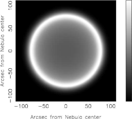
Figure 18: Contour map of $\rm{\it I}$ particularized to simulate A39.

The effect of the insertion of a threshold intensity , $\rm I_{tr}$, given by the observational techniques , is now analyzed. The threshold intensity can be parametrized to $\rm I_{max}$, the maximum value of intensity characterizing the ring: a typical image with a hole is visible in Figure 19 when $\rm I_{tr}=I_{max}/2$.

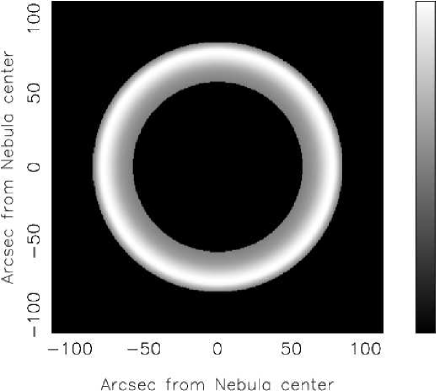
Figure 19: The same as Figure 18 but with $\rm I_{tr}=I_{max}/2$

The position of the minimum of $\rm{\it I}$ is at $\rm y=0$ and the position of the maximum is situated at $\rm y=b$.

The ratio between the theoretical intensity at maximum , $\rm I_{max}$ at $\rm y=b$ , and at the minimum ($\rm y=0$) is given by

$$\frac{I_{max}}{I(y=0)}=\frac{Numerator}{Denominator}\quad,$$ (62)

where

$$\rm\displaystyle Numerator=({b}^{2}-2\,ba+{a}^{2})$$

$$\rm\displaystyle\times(2\,cb\ln(b)-2\,c\ln(\sqrt{{c}^{2}-{b}^{2}}+c)b+b\sqrt{{c}^{2}-{b}^{2}}+{c}^{2}\arctan({\frac{\sqrt{{c}^{2}-{b}^{2}}}{b}}))\quad,$$ (63)

and

$$\rm\displaystyle Denominator=$$

$$\rm\displaystyle 2\,b({a}^{2}c-{c}^{2}a-2\,bca\ln(a)+2\,bca\ln(c)-b{a}^{2}+b{c}^{2}-{b}^{2}c+{b}^{2}a+{b}^{2}a\ln(a)$$

$$\rm\displaystyle-{c}^{2}a\ln(b)+{b}^{2}c\ln(b)-{b}^{2}a\ln(b)-{b}^{2}c\ln(c)+{a}^{2}c\ln(b)+{c}^{2}a\ln(a)-{a}^{2}c\ln(c))\quad.$$ (64)

The ratio rim(maximum) /center(minimum) of the observed intensities as well as the theoretical one are reported in Table 7.

Up to now we have not described the fainter halo of A39 which according to Jacoby et al. (2001) extends $\rm 15^{\prime\prime}$ beyond the rim. The halo intensity can be modeled by introducing two different processes of diffusion characterized by different geometrical situations . The first is represented by $\rm{\it I}$ made by the three pieces ( 5.4), ( 5.4) and ( 5.4), the second one is the intensity between a larger sphere ( $\rm r=2\times c$) and smaller sphere ( $\rm r=b$) with constant density , see formula (55 )

$$I=I(C_{m,1},a_{1},b_{1},c_{1},y)+I_{0a}(C_{m,2},a_{2},b_{2},y)\quad,$$ (65)

where the numbers 1 and 2 stand for first process and second process . The second process with constant density will be characterized by a larger volume of the considered bigger sphere and smaller number density , i.e. $\rm C_{m,2}\ll C_{m,1}$ . A typical result of this two phase process is plotted in Figure 20 and the image reported in Figure 21 ; the adopted parameters are reported in Table 8.

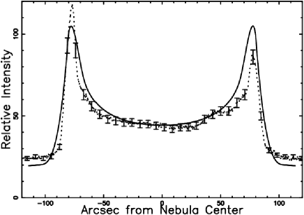
Figure 20: Cut of the mathematical intensity $\rm{\it I}$ that characterizes the two-phase diffusion ( full line ) and real data of A39 (dotted line with some error bar). The number of data is 801 and for this model $\rm\chi^{2}$ = 2.29 against $\rm\chi^{2}$ = 12.606 of the rim model fully described in  Jacoby et al. (2001).

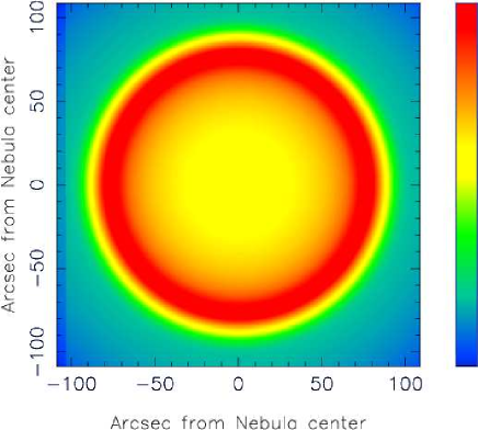
Figure 21: Contour map of the decimal logarithm of $\rm{\it I}$ of the two-phase diffusion relative to A39.

Table 8: Simulation of A39 , halo comprised

$$\rm\rm\begin{array}[]{llc}\hline\cr\hline\cr\vskip 3.0pt plus 1.0pt minus 1.0pt\cr symbol&meaning&value\\ \vskip 3.0pt plus 1.0pt minus 1.0pt\cr\hline\cr\vskip 3.0pt plus 1.0pt minus 1.0pt\cr a_{1}&radius~{}of~{}the~{}internal~{}absorbing~{}sphere&66.3^{\prime\prime}\\ \vskip 3.0pt plus 1.0pt minus 1.0pt\cr b_{1}&radius~{}of~{}the~{}shock&80^{\prime\prime}\\ \vskip 3.0pt plus 1.0pt minus 1.0pt\cr c_{1}&radius~{}of~{}the~{}external~{}absorbing~{}sphere&103.5^{\prime\prime}\\ \vskip 3.0pt plus 1.0pt minus 1.0pt\cr C_{m,1}&maximum~{}numberdensity~{}main~{}diffusion&1\\ \vskip 3.0pt plus 1.0pt minus 1.0pt\cr a_{2}&internal~{}radius~{}of~{}the~{}halo~{}process&80^{\prime\prime}\\ \vskip 3.0pt plus 1.0pt minus 1.0pt\cr b_{2}&external~{}radius~{}of~{}the~{}halo~{}process&207^{\prime\prime}\\ \vskip 3.0pt plus 1.0pt minus 1.0pt\cr C_{m,2}&numberdensity~{}halo&0.045\\ \vskip 3.0pt plus 1.0pt minus 1.0pt\cr\frac{I_{limb}}{I_{center}}&ratio~{}of~{}simulated~{}intensities&2.85\\ \vskip 3.0pt plus 1.0pt minus 1.0pt\cr\hline\cr\hline\cr\end{array}$$

5.5 3D diffusion from a sphere with drift

The influence of advection on diffusion can be explored assuming that in 3D the number density scales in the radial direction as does the 1D solution with drift represented by formulas (39) and (40) . This is an approximation due to the absence of Fick’s second equation in 3D. Also here the geometry of the phenomena fixes three different zones ($\rm 0-a,a-b,b-c$) in the variable $\rm y$ , see Figure 16, and the intensity along the line of sight can be found by imposing $\rm r=\sqrt{x^{2}+y^{2}}$ . In this case, the integral operation of the square of the number density which gives the intensity can be performed only numerically , see Figure 22.

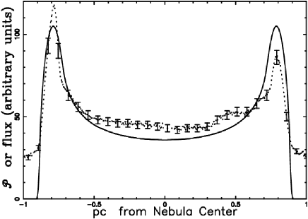
Figure 22: Cut of the numerical intensity $\rm{\it I}$ crossing the center (dotted line ) of A39 when the drift is considered and real data (full line). The parameters are $\rm u=1$ , $\rm a=69.6~{}arcsec$, $\rm b=87~{}arcsec$ , $\rm c=89~{}arcsec$ and $\rm D=6$. In this case $\rm\frac{I_{max}}{I(y=0)}$=2.92 . The number of data is 801 and for this model $\rm\chi^{2}$ = 20.96 against $\rm\chi^{2}$ = 10.36 of the rim model fully described in  Jacoby et al. (2001). The conversion from $\rm arcsec$ to $\rm pc$ is done assuming a distance of 2100 $\rm pc$ for A39.

5.6 3D complex morphologies

The numerical approach to the intensity map can be implemented when the ellipsoid that characterizes the expansion surface of the PN has a constant thickness expressed , for example , as $\rm r_{min}/f$ where $\rm r_{min}$ is the minimum radius of the ellipsoid and $\rm f$ an integer. We remember that $\rm f=12$ has a physical basis in the symmetrical case , see McCray & Layzer (1987). The numerical algorithm that allows us to build the image is now outlined

• A memory grid $\rm{\mathcal{M}}(i,j,k)$ that contains $\rm NDIM^{3}$ pixels is considered

• The points of the thick ellipsoid are memorized on $\rm{\mathcal{M}}$

• Each point of $\rm{\mathcal{M}}$ has spatial coordinates $\rm x,y,z$ which can be represented by the following $\rm 1\times 3$ matrix ,$\rm A$,

  $$A=\left[\begin{array}[]{c}x\\ \vskip 6.0pt plus 2.0pt minus 2.0pt\cr y\\ \vskip 6.0pt plus 2.0pt minus 2.0pt\cr{\it z}\end{array}\right]\quad.$$ (66)

  The point of view of the observer is characterized by the Eulerian angles $\rm(\Phi,\Theta,\Psi)$ and therefore by a total rotation $\rm 3\times 3$ matrix , $\rm E$ , see Goldstein et al. (2002). The matrix point is now represented by the following $\rm 1\times 3$ matrix , $\rm B$,

  $$B=E\cdot A\quad.$$ (67)

• The map in intensity is obtained by summing the points of the rotated images along a direction , for example along z , ( sum over the range of one index, for example k ).

Figure 23 reports the rotated image of the Ring nebula and Figure 24 reports two cuts along the polar and equatorial directions.

Figure 25 reports the comparison between a theoretical and observed east-west cut in $\rm H_{\beta}$ that cross the center of the nebula, see Figure 1 in Garnett & Dinerstein (2001).

A comparison can be made with the color composite image of Doppler-shifted $\rm H_{2}$ emission as represented in Figure 2 in Hiriart (2004).

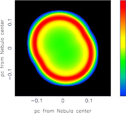
Figure 23: Map of the theoretical intensity of the Ring nebula. Physical parameters as in Table 1 and $\rm f$=12 . The three Eulerian angles characterizing the point of view are $\rm\Phi$=180 ^∘, $\rm\Theta$=90 ^∘ and $\rm\Psi$=-30 ^∘.

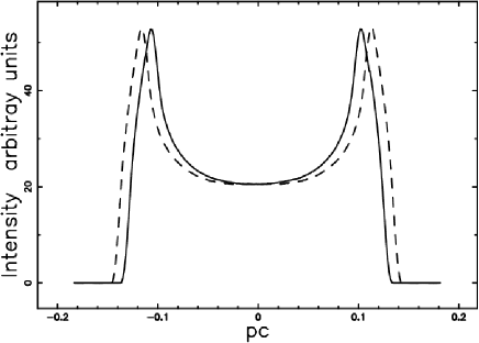
Figure 24: Two cut of the mathematical intensity $\rm{\it I}$ crossing the center of the Ring nebula: equatorial cut (full line) and polar cut (dotted line) .

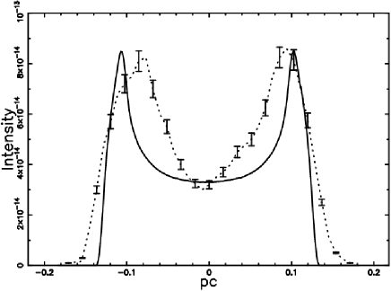
Figure 25: Cut of the mathematical intensity $\rm{\it I}$ of the Ring Nebula crossing the center (full line ) and real data of $\rm H_{\beta}$ (dotted line with some error bar ) . The number of data is 250 and for this model $\rm\chi^{2}$ = 15.53 . The real data are extracted by the author from Figure 1 of Garnett and Dinerstein 2001.

In order to explain some of the morphologies which characterize the PN’s we first map MyCn 18 with the polar axis in the vertical direction , see map in intensity in Figure 26. The vertical and horizontal cut in intensity are reported in Figure 28. The point of view of the observer as modeled by the Euler angles increases the complexity of the shapes : Figure 27 reports the after rotation image and Figure 29 the vertical and horizontal rotated cut. The after rotation image contains the double ring and an enhancement in intensity of the central region which characterize MyCn 18.

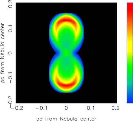
Figure 26: Map of the theoretical intensity of MyCn 18 . Physical parameters as in Table 4 and $\rm f$=12 . The three Eulerian angles characterizing the point of view are $\rm\Phi$=180 ^∘ , $\rm\Theta$=90 ^∘ and $\rm\Psi$=0 ^∘.

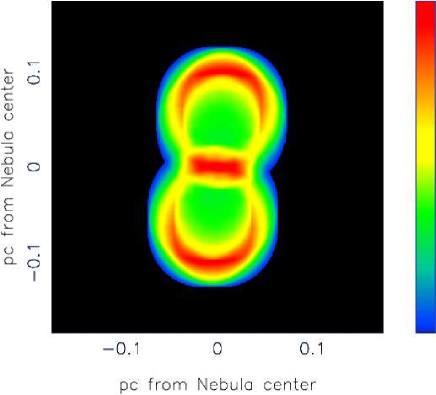
Figure 27: Map of the theoretical intensity of the rotated MyCn 18 . Physical parameters as in Table 4 and $\rm f$=12 . The three Eulerian angles characterizing the point of view are $\rm\Phi$=130 ^∘, $\rm\Theta$=40 ^∘ and $\rm\Psi$=5 ^∘.

This central enhancement can be considered one of the various morphologies that the PNs present and is similar to model $\rm BL_{1}-F$ in Figure 3 of the Atlas of synthetic line profiles by Morisset & Stasinska (2008).

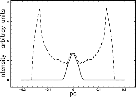
Figure 28: Two cut of the mathematical intensity $\rm{\it I}$ crossing the center of MyCn 18 : equatorial cut (full line) and polar cut (dotted line) . Parameters as in Figure 26.

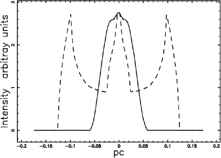
Figure 29: Two cut of the mathematical intensity $\rm{\it I}$ crossing the center of the rotated MyCn 18 nebula: equatorial cut (full line) and polar cut (dotted line) . Parameters as in Figure 27.

6 Conclusions

Law of motion The law of motion in the case of a symmetric motion can be modeled by the Sedov Solution or the radial momentum conservation. These two models allow to determine the approximate age of A39 which is 8710 $\rm yr$ for the Sedov solution and 50000 $\rm yr$ for the radial momentum conservation. In presence of gradients as given , for example , by an exponential behavior, the solution is deduced through the radial momentum conservation. The comparison with the astronomical data is now more complicated and the single and multiple efficiency in the radius determination have been introduced. When , for example , MyCn 18 is considered , the multiple efficiency over 18 directions is $\rm 90.66\%$ when the age of 2000 $\rm yr$ is adopted.

Diffusion

The number density in a thick layer surrounding the ellipsoid of expansion can be considered constant or variable from a maximum value to a minimum value with the growing or diminishing radius in respect to the expansion position. In the case of a variable number density the framework of the mathematical diffusion has been adopted, see formulas (34) and  (35). The case of diffusion with drift has been analytically solved , see formulas (39) and  (40), and the theoretical formulas have been compared with values generated by Monte Carlo simulations.

Images

The intensity of the image of a PN when the intensity of emission is proportional to the square of the number density can be computed through

• an analytical evaluation of lines of sight when the number density is constant between two spheres or in one sphere , see formula (55) and formula (58).

• analytical evaluation of integrals when the number density is variable , see formulas ( 5.4), ( 5.4) and ( 5.4), when the motion is symmetric. In this framework it is also possible to build a two-phase diffusion model that allows us to reproduce the faint extended halo, see formula (65).

• a numerical evaluation of integrals when the number density is variable , the drift is present and the motion is symmetric, see Section 5.5.

• a numerical evaluation of lines of sight when the motion is asymmetric, see Section 5.6.

In the case of A39 the $\rm\chi^{2}$ of comparison between the theoretical and observed cut in intensity can be evaluated , see Table 9. From a careful evaluation of Table 9 it is possible to conclude that the models here considered produce $\rm\chi^{2}$ which are slightly bigger than the rim model of Jacoby et al. (2001). When , conversely , a diffuse halo is considered the $\rm\chi^{2}$ is smaller ; this makes the study of the interaction between PN and the surrounding halo an interesting field of research.

Next step

Here we have explored the conservation of the radial momentum in a medium with an exponential behavior of the type $\rm\rho\propto\exp{-\frac{R\times\sin(\theta)}{h}}$ which is symmetric in respect to the plane $\rm z=0$ . The next target can be the analysis of the conservation of the radial momentum in a spherical symmetry of the type $\rm\rho\propto R^{-\alpha}$ , see Section 1. In this case the spatially asymmetric motion can be obtained by considering the conservation of the radial momentum in a medium with density of the type $\rm\rho\propto R^{-\alpha}\times\exp{-\frac{R\times\sin(\theta)}{h}}$.

Table 9: Data of the simulation of the Ring nebula

$$\rm\rm\begin{array}[]{lcc}\hline\cr\vskip 3.0pt plus 1.0pt minus 1.0pt\cr model&\mbox{ $\rm\chi^{2}$}&\mbox{ $\rm\chi^{2}$ }~{}of~{}reference,~{}Jacoby~{}et~{}al.~{}2001\\ rim~{}with~{}fixed~{}thickness&1.487&0.862\\ diffusion&19.03&12.60\\ diffusion~{}with~{}drift&20.96&10.36\\ diffusion~{}+~{}halo&2.29&12.606\\ \vskip 3.0pt plus 1.0pt minus 1.0pt\cr\hline\cr\end{array}$$

References

- Balick (1987) Balick B., 1987, AJ, 94, 671
- Berg (1993) Berg H. C., 1993, Random Walks in Biology. Princeton University Press, Princeton
- Blagrave et al. (2006) Blagrave K. P. M., Martin P. G., Baldwin J. A., 2006, ApJ , 644, 1006
- Cohen et al. (2006) Cohen M., Chapman J. M., Deacon R. M., Sault R. J., Parker Q. A., Green A. J., 2006, MNRAS , 369, 189
- Corradi & Schwarz (1993) Corradi R. L. M., Schwarz H. E., 1993, A&A , 278, 247
- Crank (1979) Crank J., 1979, Mathematics of Diffusion. Oxford University Press, Oxford
- Dayal et al. (2000) Dayal A., Sahai R., Watson A. M., Trauger J. T., Burrows C. J., Stapelfeldt K. R., Gallagher III J. S., 2000, AJ, 119, 315
- Dyson & Williams (1997) Dyson J. E., Williams D. A., 1997, The physics of the interstellar medium. Institute of Physics Publishing, Bristol
- Frank et al. (1995) Frank A., Balick B., Davidson K., 1995, ApJ , 441, L77
- Garnett & Dinerstein (2001) Garnett D. R., Dinerstein H. L., 2001, ApJ , 558, 145
- Goldstein et al. (2002) Goldstein H., Poole C., Safko J., 2002, Classical mechanics. Addison-Wesley, San Francisco
- González et al. (2004) González R. F., de Gouveia Dal Pino E. M., Raga A. C., Velazquez P. F., 2004, ApJ , 600, L59
- González et al. (2006) González R. F., Montes G., Cantó J., Loinard L., 2006, MNRAS , 373, 391
- Gruenwald & Aleman (2007) Gruenwald R., Aleman A., 2007, A&A , 461, 1019
- Guerrero et al. (2004) Guerrero M. A., Jaxon E. G., Chu Y.-H., 2004, AJ, 128, 1705
- Harris et al. (1997) Harris H. C., Dahn C. C., Monet D. G., Pier J. R., 1997, in Habing H. J., Lamers H. J. G. L. M., eds, Planetary Nebulae Vol. 180 of IAU Symposium, Trigonometric parallaxes of Planetary Nebulae (Invited Review). pp 40–+
- Hippelein & Weinberger (1990) Hippelein H., Weinberger R., 1990, A&A , 232, 129
- Hiriart (2004) Hiriart D., 2004, PASP, 116, 1135
- Hjellming (1988) Hjellming R. M., 1988, Radio stars. Galactic and Extragalactic Radio Astronomy, pp 381–438
- Icke (1988) Icke V., 1988, A&A , 202, 177
- Jacoby et al. (2001) Jacoby G. H., Ferland G. J., Korista K. T., 2001, ApJ , 560, 272
- Kahn & West (1985) Kahn F. D., West K. A., 1985, MNRAS , 212, 837
- Kim et al. (2000) Kim J., Franco J., Hong S. S., Santillán A., Martos M. A., 2000, ApJ , 531, 873
- Kwok et al. (1978) Kwok S., Purton C. R., Fitzgerald P. M., 1978, ApJ , 219, L125
- Lang (1999) Lang K. R., 1999, Astrophysical formulae. (Third Edition). Springer, New York
- Langer et al. (1999) Langer N., García-Segura G., Mac Low M.-M., 1999, ApJ , 520, L49
- Manchado et al. (1996) Manchado A., Stanghellini L., Guerrero M. A., 1996, ApJ , 466, L95+
- Matsumoto et al. (2006) Matsumoto H., Fukue T., Kamaya H., 2006, PASJ , 58, 861
- McCray & Layzer (1987) McCray R. In: Dalgarno A., Layzer D., eds, 1987, Spectroscopy of astrophysical plasmas Cambridge University Press
- Mellema et al. (1991) Mellema G., Eulderink F., Icke V., 1991, A&A , 252, 718
- Morisset & Stasinska (2008) Morisset C., Stasinska G., 2008, Revista Mexicana de Astronomia y Astrofisica, 44, 171
- Padmanabhan (2001) Padmanabhan P., 2001, Theoretical astrophysics. Vol. II: Stars and Stellar Systems. Cambridge University Press, Cambridge, MA
- Perinotto et al. (2004) Perinotto M., Schönberner D., Steffen M., Calonaci C., 2004, A&A , 414, 993
- Press et al. (1992) Press W. H., Teukolsky S. A., Vetterling W. T., Flannery B. P., 1992, Numerical recipes in FORTRAN. The art of scientific computing. Cambridge University Press, Cambridge
- Rybicki & Lightman (1985) Rybicki G., Lightman A., 1985, Radiative Processes in Astrophysics. Wiley-Interscience, New-York
- Sabbadin et al. (1984) Sabbadin F., Gratton R. G., Bianchini A., Ortolani S., 1984, A&A , 136, 181
- Sahai et al. (1999) Sahai R., Dayal A., Watson A. M., Trauger J. T., Stapelfeldt K. R., Burrows C. J., Gallagher III J. S., Scowen P. A., Hester J. J., Evans R. W., Ballester G. E., Clarke J. T., Crisp D., Griffiths R. E., Hoessel J. G., Holtzman J. A., Krist J., Mould J. R., 1999, AJ, 118, 468
- Schönberner et al. (2005) Schönberner D., Jacob R., Steffen M., 2005, A&A , 441, 573
- Schönberner et al. (2005) Schönberner D., Jacob R., Steffen M., Perinotto M., Corradi R. L. M., Acker A., 2005, A&A , 431, 963
- Schönberner et al. (2007) Schönberner D., Jacob R., Steffen M., Sandin C., 2007, A&A , 473, 467
- Schwarz et al. (1992) Schwarz H. E., Corradi R. L. M., Melnick J., 1992, A&AS, 96, 23
- Schwarz & Monteiro (2006) Schwarz H. E., Monteiro H., 2006, ApJ , 648, 430
- Sedov (1959) Sedov L. I., 1959, Similarity and Dimensional Methods in Mechanics. Academic Press, New York
- Soker (2002) Soker N., 2002, MNRAS , 330, 481
- Soker & Hadar (2002) Soker N., Hadar R., 2002, MNRAS , 331, 731
- Steffen et al. (2008) Steffen M., Schönberner D., Warmuth A., 2008, A&A , 489, 173
- Tsui (2008) Tsui K. H., 2008, A&A , 482, 793
- Villaver et al. (2002) Villaver E., Manchado A., García-Segura G., 2002, ApJ , 581, 1204
- Zaninetti (2007) Zaninetti L., 2007, Baltic Astronomy, 16, 251