Retarded Casimir-Polder force on an atom near reflecting microstructures

Abstract

We derive the fully retarded energy shift of a neutral atom in two different geometries useful for modelling etched microstructures. First we calculate the energy shift due to a reflecting cylindrical wire, and then we work out the energy shift due to a semi-infinite reflecting half-plane. We analyze the results for the wire in various limits of the wire radius and the distance of the atom from the wire, and obtain simple asymptotic expressions useful for estimates. For the half-plane we find an exact representation of the Casimir-Polder interaction in terms of a single, fast converging integral, which is easy to evaluate numerically.

I INTRODUCTION

The explosive rate of developments in nanotechnology as well as in the manipulation of cold atoms has meant that interest in atom-surface interactions has increased strongly in recent years. What were once tiny, elusive effects are now dominant interactions, or, as the case may be, a major nuisance in some experimental set-ups. Motivated by a common type of microstructure, which consists of a protruding ledge fabricated by successive etching and possibly a thin electroplated top layer, we have recently studied the force on a neutral atom in close proximity of reflecting surfaces of either cylindrical geometry or that of a semi-infinite half-plane nonret . In the absence of free charges or thermal excitations, the interaction of the atom with the microstructure is dominated by Casimir-Polder forces casimir , which are due to the interaction of the atomic dipole with polarization fluctuations excited by vacuum fluctuations of the electromagnetic field. If the atom is sufficiently close to the surface of the microstructure, then the interaction between the atomic dipole and the surface is purely electrostatic and retardation can be neglected, which was the case investigated in Ref. nonret . Then one does not need to quantize the electromagnetic field, but can work with the classical Green’s function of Poisson’s equation. The only difficulty lies then in the geometry of the problem.

However, in experimental situations one more often finds that retardation is in fact important, as the distance of the atom from the surface of the microstructure is often commensurate or larger than the wavelength of a typical atomic transition. This is the case we investigate here, again for microstructures of two types of geometries: a cylindrical reflector of radius $R$ and infinite length, and a reflecting half-plane.

Various versions of this problem have been studied before, both analytically and numerically. Probably the first to consider the interaction between an atom and a metallic wire, according to Barash , was almost 75 years ago Zel’dovich Zeldovich . This problem was then revisited and extended by Nabutovskii et al. Nabutovskii , and subsequently by Marvin et al. Marvin . In Nabutovskii’s paper a dielectric cylinder is envisaged to be surrounded by a cylindrical shell of vacuum which in turn is surrounded by a rarefied gas of polarizable particles. The interaction energy of a single particle is then calculated through the work done by the force (obtained from the stress tensor) due to the fluctuating electromagnetic fields, in the limit of zero density of the surrounding gas. The asymptotic results obtained there (Eq. (23) and Eq. (24) of Ref. Nabutovskii ) are, according to Ref. Barash , valid only for dilute dielectric materials; they diverge in the perfect-reflector limit.

On the other hand, the work by Marvin et al.Marvin , motivated by Mehl1 ; Mehl2 and based on a normal-mode expansion and a linear-response formalism Langbein , gives the same general formula for the interaction between a point particle and a cylinder [their Eq. (4.10)] as the equivalent result in Nabutovskii . We have no reason to believe that the result in Marvin is incorrect in the perfect-conductor limit, as it reduces to our previous result nonret in the electrostatic limit. Moreover, Ref. Marvin manages to recover the original Casimir-Polder result casimir in the large-radius limit of the cylinder. This suggests that the general expression in Nabutovskii is probably correct, only that the perfect-conductor limit does not commute with the asymptotic limit of the zero radius (or large distance of the atom from the cylinder) studied there. In the small-radius limit, the result for the interaction between an atom and a metallic filament, in both retarded and non-retarded limits, is also given by Barash .

Marvin et al.’s work Marvin is certainly the most comprehensive, but due to its generality it is also quite cumbersome to apply, which is mainly done numerically for just a few examples Marvin2 . Further numerical studies of the interaction of atoms with macroscopic cylinders can be found in Refs. Fussell ; Boustimi1 ; Boustimi2 ; Blagov .

By contrast, in this paper we are after a relatively simple theory that allows one to estimate the force between an atom and a cylindrical reflector at any distance and cylinder radius. To this end we are not interested in the precise dependence of the interaction on material constants of the reflector, and therefore we work with the model of a perfectly reflecting surface.

As discussed in Ref. nonret , we also determine the force between an atom and a semi-infinite half-plane, in order to facilitate estimates for common types of microstructures that consist of a ledge protruding from a substrate. The Casimir-Polder interaction between an atom and such a half-plane has also studied before, but only in the extreme retarded limit of very large distances of the atom from the surface Brevik . To the best of our knowledge no formula for the interaction in the intermediate region, when the distance of the atom from the surface is comparable to the typical wavelength of an internal transition in the atom, has been derived yet. Recent work of Mendes et al. Farina2 , dealing with wedges, does not include the general result in the half-plane geometry as a limiting case of a zero-angle wedge.

II FIELD QUANTIZATION AND THE ENERGY SHIFT

The complete system of an atom interacting with the quantized electromagnetic field is described by the Hamiltonian

$$H=H_{\rm{Atom}}+H_{\rm{Field}}+H_{\rm{Int}}\;.$$ (1)

We choose to work with $\boldsymbol{\mu}\cdot{\bf E}$ coupling, i.e. our interaction Hamiltonian is

$$H_{\rm{Int}}=-\boldsymbol{\mu}\cdot{\bf E}\;.$$ (2)

Quantization of the electromagnetic field is done by way of a normal-mode expansion of the vector potential in terms of photon annihilation and creation operators for each mode $\lambda$ and polarization $\sigma$,

$$\mathbf{A}(\mathbf{r},t)=\sum_{\lambda,\sigma}\frac{1}{\sqrt{2\varepsilon_{0}\omega_{\lambda}}}\left[a_{\lambda}^{(\sigma)}{\bf F}_{\lambda}^{(\sigma)}(\mathbf{r})\;e^{-{\rm i}\omega t}+\mbox{h.c.}\right].$$ (3)

To describe a mode we use the composite index $\lambda$ instead of a wave vector, as we shall be working in cylindrical coordinates where the quantum number of the azimuthal part of the mode function is discrete, but the other two are continuous. We work in Coulomb gauge, $\boldsymbol{\nabla}\cdot{\bf A}(\mathbf{r})$, so that the normal modes ${\bf F}(\mathbf{r})$ satisfy the Helmholtz equation,

$$(\boldsymbol{\nabla}^{2}+\omega^{2})\,\mathbf{F}(\mathbf{r})=0\;.$$ (4)

The energy level shift due to the interaction (2) can be calculated perturbatively. For our system in state $|i;0\rangle$, i.e. the atom in state $|i\rangle$ and the electromagnetic field in its vacuum state $|0\rangle$, the lowest non-vanishing order of perturbation theory is the second, so that

$$\Delta W=\sum_{j\neq i}\frac{\left|\left\langle j;1_{\lambda}^{(\sigma)}\left|-\boldsymbol{\mu}\cdot{\bf E}\right|i;0\right\rangle\right|^{2}}{E_{i}-(E_{j}+\omega_{\lambda})}\;.$$ (5)

As the relevant field modes can be expected to vary slowly over the size of the atom, we make the electric dipole approximation, which simplifies the expression for the energy shift to

$$\Delta W=-\sum_{\lambda,\sigma,j\neq i}\frac{\omega_{\lambda}}{2\varepsilon_{0}}\;\frac{\left|\langle j|\boldsymbol{\mu}|i\rangle\cdot{\bf F}^{(\sigma)*}_{\lambda}(\mathbf{r})\right|^{2}}{E_{ji}+\omega_{\lambda}}\;,$$ (6)

where we have introduced the abbreviation $E_{ji}\equiv E_{j}-E_{i}$. For brevity and presentational clarity we shall henceforth also abbreviate the matrix elements of the atomic dipole moment as

$$\left|\boldsymbol{\mu}\right|\equiv\left|\left\langle j\left|\boldsymbol{\mu}\right|i\right\rangle\right|\;.$$ (7)

III ENERGY SHIFT NEAR A PERFECTLY REFLECTING WIRE

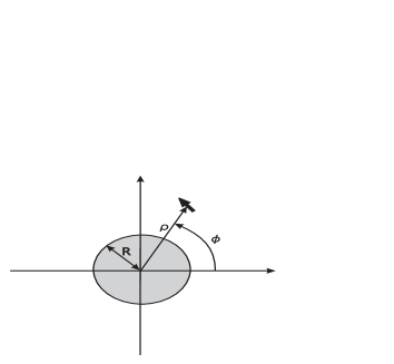
Figure 1: Atomic electric dipole moment in the vicinity of a perfectly reflecting cylinder of radius $R$. The normal modes $\mathbf{F}_{\lambda}^{(\sigma)}(\mathbf{x})$ in this geometry are given by Eqs. (13) and (14).

First we wish to calculate the energy shift of an atom near a perfectly reflecting and infinitely long cylindrical wire of radius $R$. It is advantageous to work in cylindrical coordinates, cf. Fig. 1.

In order to find two independent transverse vector field solutions of Eq. (4), we make use of the representation theorem for the vector Helmholtz equation (GR, , 10.411). If $\Phi(\mathbf{x})$ is a solution of the scalar Helmholtz equation then the two independent solutions of the vector equation are given by

$$\mathbf{F}^{(1)}(\mathbf{r}) \!\!= \!\!\left(\mathbf{\nabla}\times\hat{\mathbf{e}}_{z}\right)\Phi(\mathbf{r})\;,$$ (8)

$$\mathbf{F}^{(2)}(\mathbf{r}) \!\!= \!\!\frac{1}{\omega}\mathbf{\nabla}\times\left(\mathbf{\nabla}\times\hat{\mathbf{e}}_{z}\right)\Phi(\mathbf{r})\;.$$ (9)

The particular choice of the constant unit vector $\hat{\mathbf{e}}_{z}$ is motivated by the symmetry of our problem and lets us to identify the solutions $\mathbf{F}^{(1)}(\mathbf{r})$ and $\mathbf{F}^{(2)}(\mathbf{r})$ with the transverse electric (TE) and transverse magnetic (TM) modes, respectively. In cylindrical coordinates the scalar Helmholtz equation has the solutions of the form

$$\Phi(\rho,\phi,z)=N\left[\;\cos\delta_{m}J_{m}(k\rho)+\sin\delta_{m}Y_{m}(k\rho)\;\right]e^{{\rm i}m\phi+{\rm i}\kappa z}$$ (10)

where $J_{m}(k\rho)$ and $Y_{m}(k\rho)$ are Bessel functions of the first and second kind (AS, , §9). The separation constants satisfy $\omega^{2}=k^{2}+\kappa^{2}$, and $m$ is an integer. The phase shifts $\delta_{m}$ describe the superposition of regular and irregular solutions. In free space only regular solutions $J_{m}(k\rho)$ are admissible, and $\delta_{m}=0$. In the presence of the perfectly reflecting wire, the phase shifts serve to make the electromagnetic fields satisfy the boundary conditions on the surface of the wire. The normalization constant $N$ is chosen such that

$$\int\mathrm{d}^{3}\mathbf{r}\;\mathbf{F}^{(\sigma)*}_{\lambda^{\prime}}(\mathbf{r})\cdot\mathbf{F}^{(\sigma)}_{\lambda}(\mathbf{r})=\delta_{mm^{\prime}}\delta(\kappa-\kappa^{\prime})\frac{\delta{(k-k^{\prime})}}{\sqrt{kk^{\prime}}}$$ (11)

is met. Setting $\cos\delta_{m}=1$, $\sin\delta_{m}=0$, one can derive quite easily that $N=(2\pi k)^{-1}$.

On the surface of a perfect conductor, the tangential components of the electric field and the normal component of the magnetic field vanish. Therefore, at the surface $\rho=R$ of the cylindrical wire we must have $E_{\phi}=0=E_{z}$ and $B_{\rho}=0.$ These boundary conditions determine the phase shifts as

$$\tan\delta_{m}^{\text{TE}}=-\frac{J^{\prime}_{m}(kR)}{Y^{\prime}_{m}(kR)},\;\tan\delta_{m}^{\text{TM}}=-\frac{J_{m}(kR)}{Y_{m}(kR)}\;.$$ (12)

According to Eqs. (8), (9), and (10), the normalized mode functions $\mathbf{F}_{\lambda}^{(\sigma)}(\mathbf{r})$, $\lambda=\{k,m,\kappa\}$, that satisfy the boundary conditions at $\rho=R$ are given by

$$\mathbf{F}_{\lambda}^{\text{TE}}(\rho,\phi,z)$$

$$=\frac{1}{2\pi}\left[\frac{{\rm i}m}{k\rho}\frac{J_{m}(k\rho)Y^{\prime}_{m}(kR)-Y_{m}(k\rho)J^{\prime}_{m}(kR)}{\sqrt{J_{m}^{{}^{\prime}2}(kR)+Y_{m}^{{}^{\prime}2}(kR)}}\;\hat{\mathbf{e}}_{\rho}\right.$$ (13)

$$\ \ \ -\left.\frac{J^{\prime}_{m}(k\rho)Y^{\prime}_{m}(kR)-Y^{\prime}_{m}(k\rho)J^{\prime}_{m}(kR)}{\sqrt{J^{{}^{\prime}2}_{m}(kR)+Y^{{}^{\prime}2}_{m}(kR)}}\;\hat{\mathbf{e}}_{\phi}\right]e^{{\rm i}m\phi+{\rm i}\kappa z},$$

$$\mathbf{F}_{\lambda}^{\text{TM}}(\rho,\phi,z)$$

$$=\frac{1}{2\pi}\left[\frac{i\kappa}{\omega}\frac{J^{\prime}_{m}(k\rho)Y_{m}(kR)-Y^{\prime}_{m}(k\rho)J_{m}(kR)}{\sqrt{J_{m}^{2}(kR)+Y_{m}^{2}(kR)}}\;\hat{\mathbf{e}}_{\rho}\right.$$

$$\ \ \ -\frac{m\kappa}{\omega k\rho}\frac{J_{m}(k\rho)Y_{m}(kR)-Y_{m}(k\rho)J_{m}(kR)}{\sqrt{J_{m}^{2}(kR)+Y_{m}^{2}(kR)}}\;\hat{\mathbf{e}}_{\phi}$$ (14)

$$\ \ \ +\left.\frac{k}{\omega}\frac{J_{m}(k\rho)Y_{m}(kR)-Y_{m}(k\rho)J_{m}(kR)}{\sqrt{J_{m}^{2}(kR)+Y_{m}^{2}(kR}}\;\hat{\mathbf{e}}_{z}\right]e^{{\rm i}m\phi+{\rm i}\kappa z}.$$

These mode functions can now be substituted into Eq. (6) for obtaining the energy shift of an atom positioned at $\mathbf{r}=(\rho,\phi,z)$. However, what we want to calculate here is only the correction to the energy shift caused by the presence of a perfectly conducting surface, rather than the whole energy shift due to the coupling of the atom to the fluctuating vacuum field, which would include the free-space Lamb shift. Therefore we need to subtract the energy shift caused by the vacuum fluctuations of the electromagnetic field in free space, which is obtained by either letting the phase shifts $\delta_{m}\rightarrow 0$ or equivalently taking the limit $R\rightarrow 0$. In the limit of vanishing radius $R$ of the cylinder the behaviour of the mode functions (13), (14) is dominated by the singular behaviour of $Y_{m}(kR)$ and $Y^{\prime}_{m}(kR)$ at the origin, which causes the phase shifts (12) to vanish. The renormalized energy shift $\Delta W^{\rm{ren}}=\Delta W-\lim_{R\rightarrow 0}\Delta W$ is found to be of the form

$$\Delta W^{\rm{ren}}=-\frac{1}{4\pi\varepsilon_{0}}\sum_{j\neq i}\left(\Xi_{\rho}|\mu_{\rho}|^{2}+\Xi_{\phi}|\mu_{\phi}|^{2}+\Xi_{z}|\mu_{z}|^{2}\right)$$ (15)

with

$$\Xi_{\rho} \!\!= \!\!\frac{2}{\pi}\sum_{m=0}^{\infty}\!\!\text{ }^{\prime}\int_{0}^{\infty}\mathrm{d}k\;k\int_{0}^{\infty}\mathrm{d}\kappa\;\frac{\omega}{E_{ji}+\omega}\left\{\left(\frac{m}{k\rho}\right)^{2}\left[\frac{\big{(}J_{m}(k\rho)Y^{\prime}_{m}(kR)-Y_{m}(k\rho)J^{\prime}_{m}(kR)\big{)}^{2}}{J^{{}^{\prime}2}_{m}(kR)+Y^{{}^{\prime}2}_{m}(kR)}-J^{2}_{m}(k\rho)\right]\right.$$ (16)

$$\hskip 99.58464pt+\left.\left(\frac{\kappa}{\omega}\right)^{2}\left[\frac{\big{(}J^{\prime}_{m}(k\rho)Y_{m}(kR)-Y^{\prime}_{m}(k\rho)J_{m}(kR)\big{)}^{2}}{J_{m}^{2}(kR)+Y_{m}^{2}(kR)}-J^{\prime 2}_{m}(k\rho)\right]\right\},$$

$$\Xi_{\phi} \!\!= \!\!\frac{2}{\pi}\sum_{m=0}^{\infty}\!\!\text{ }^{\prime}\int_{0}^{\infty}\mathrm{d}k\;k\int_{0}^{\infty}\mathrm{d}\kappa\;\frac{\omega}{E_{ji}+\omega}\left\{\left[\frac{\big{(}J^{\prime}_{m}(k\rho)Y^{\prime}_{m}(kR)-Y^{\prime}_{m}(k\rho)J^{\prime}_{m}(kR)\big{)}^{2}}{J^{{}^{\prime}2}_{m}(kR)+Y^{{}^{\prime}2}_{m}(kR)}-J^{\prime 2}_{m}(k\rho)\right]\right.$$ (17)

$$\hskip 99.58464pt+\left.\left(\frac{m}{k\rho}\frac{\kappa}{\omega}\right)^{2}\left[\frac{\big{(}J_{m}(k\rho)Y_{m}(kR)-Y_{m}(k\rho)J_{m}(kR)\big{)}^{2}}{J_{m}^{2}(kR)+Y_{m}^{2}(kR)}-J^{2}_{m}(k\rho)\right]\right\},$$

$$\Xi_{z} \!\!= \!\!\frac{2}{\pi}\sum_{m=0}^{\infty}\!\!\text{ }^{\prime}\int_{0}^{\infty}\mathrm{d}k\;k\int_{0}^{\infty}\mathrm{d}\kappa\;\frac{\omega}{E_{ji}+\omega}\left\{\left(\frac{k}{\omega}\right)^{2}\left[\frac{\big{(}J_{m}(k\rho)Y_{m}(kR)-Y_{m}(k\rho)J_{m}(kR)\big{)}^{2}}{J_{m}^{2}(kR)+Y_{m}^{2}(kR)}-J^{2}_{m}(k\rho)\right]\right\}$$ (18)

where the primes on the sums indicate that the ${m=0}$ term is weighted by an additional factor of 1/2. It appears that the $\kappa$ integrals fail to converge, but this is a common feature in such calculations caused by the dipole approximation, see e.g. casimir . As we shall see, convergence is in fact brought about by the Bessel functions, which come to bear if the $k$ integral is replaced by an integral over $\omega=\sqrt{\kappa^{2}+k^{2}}$.

As the Bessel functions $J_{m}(x)$ and $Y_{m}(x)$ are both oscillatory for large $x$, we wish to rotate the integration contour in the complex $k$ plane, in order to get an integrand that is exponentially damped for large arguments. To this end we introduce the Hankel functions $H_{m}^{(1)}(x)=J_{m}(x)+iY_{m}(x)$ and $H_{m}^{(2)}(x)=[H_{m}^{(1)}(x)]^{*}=J_{m}(x)-iY_{m}(x)$, in terms of which we can rewrite the energy level shift in such a form that there are no poles in the first quadrant of the complex $k$ plane, as is required for the rotation of the integration contour. This step greatly simplifies further analysis.

$$\Xi_{\rho} \!\!= \!\!-\mathrm{Re}\ \frac{2}{\pi}\sum_{m=0}^{\infty}\!\!\text{ }^{\prime}\int_{0}^{\infty}\mathrm{d}k\;k\int_{0}^{\infty}\mathrm{d}\kappa\;\frac{\omega}{E_{ji}+\omega}\left\{\frac{\kappa^{2}}{\omega^{2}}[H_{m}^{\prime(1)}(k\rho)]^{2}\frac{J_{m}(kR)}{H^{(1)}_{m}(kR)}+\frac{m^{2}}{k^{2}\rho^{2}}[H^{(1)}_{m}(k\rho)]^{2}\frac{J^{\prime}_{m}(kR)}{H_{m}^{\prime(1)}(kR)}\right\},$$ (19)

$$\Xi_{\phi} \!\!= \!\!-\mathrm{Re}\ \frac{2}{\pi}\sum_{m=0}^{\infty}\!\!\text{ }^{\prime}\int_{0}^{\infty}\mathrm{d}k\;k\int_{0}^{\infty}\mathrm{d}\kappa\;\frac{\omega}{E_{ji}+\omega}\left\{[H_{m}^{\prime(1)}(k\rho)]^{2}\frac{J^{\prime}_{m}(kR)}{H^{\prime(1)}_{m}(kR)}+\frac{m^{2}}{k^{2}\rho^{2}}\frac{\kappa^{2}}{\omega^{2}}[H^{(1)}_{m}(k\rho)]^{2}\frac{J_{m}(kR)}{H_{m}^{(1)}(kR)}\right\},$$ (20)

$$\Xi_{z} \!\!= \!\!-\mathrm{Re}\ \frac{2}{\pi}\sum_{m=0}^{\infty}\!\!\text{ }^{\prime}\int_{0}^{\infty}\mathrm{d}k\;k\int_{0}^{\infty}\mathrm{d}\kappa\;\frac{\omega}{E_{ji}+\omega}\left\{\frac{k^{2}}{\omega^{2}}[H_{m}^{(1)}(k\rho)]^{2}\frac{J_{m}(kR)}{H^{(1)}_{m}(kR)}\right\}.$$ (21)

We now transform the $k$ integration in Eqs. (19)–(21) into an integration over $\omega=\sqrt{\kappa^{2}+k^{2}}$, and note that on the interval $0\leq\omega\leq\kappa$ the integrands become pure imaginary and therefore do not contribute if added to the real part of the integral. We can therefore shift the lower limit down to the origin

$$\int_{\kappa}^{\infty}\mathrm{d}\omega\longrightarrow\int_{0}^{\infty}\mathrm{d}\omega\;$$ (22)

without affecting the result. Further, we note that the functions $H_{m}^{(1)}(z)$ and $H_{m}^{\prime(1)}(z)$ have no zeros in the first quadrant of the complex plane (AS, , Fig. 9.6), so that the contour of the $\omega$-integration can be rotated from the positive real to the positive imaginary axis, $\omega\rightarrow{\rm i}\omega$. Then the oscillatory Bessel functions turn into the modified Bessel functions according to (AS, , 9.6.3 & 5)

$$J_{m}({\rm i}z) \!\!= \!\!e^{{\rm i}m\pi/2}I_{m}(z),$$ (23)

$$H_{m}^{(1)}({\rm i}z) \!\!= \!\!-\frac{2{\rm i}}{\pi}e^{-{\rm i}m\pi/2}K_{m}(z)\;.$$ (24)

Taking the real part and going to polar coordinates, where the angle integrals are elementary, we find that

$$\Xi_{\rho} \!\!= \!\!\frac{2}{\pi}\sum_{m=0}^{\infty}\!\!\text{ }^{\prime}\int_{0}^{\infty}\mathrm{d}k\;k\left\{\left(\sqrt{E_{ji}^{2}+k^{2}}-E_{ji}\right)\frac{I_{m}(kR)}{K_{m}(kR)}[K^{\prime}_{m}(k\rho)]^{2}+\frac{m^{2}}{k^{2}\rho^{2}}\left(\frac{E_{ji}^{2}}{\sqrt{E_{ji}^{2}+k^{2}}}-E_{ji}\right)\frac{I^{\prime}_{m}(kR)}{K^{\prime}_{m}(kR)}[K_{m}(k\rho)]^{2}\right\},$$

$$\Xi_{\phi} \!\!= \!\!\frac{2}{\pi}\sum_{m=0}^{\infty}\!\!\text{ }^{\prime}\int_{0}^{\infty}\mathrm{d}k\;k\left\{\left(\frac{E_{ji}^{2}}{\sqrt{E_{ji}^{2}+k^{2}}}-E_{ji}\right)\frac{I^{\prime}_{m}(kR)}{K^{\prime}_{m}(kR)}[K^{\prime}_{m}(k\rho)]^{2}+\frac{m^{2}}{k^{2}\rho^{2}}\left(\sqrt{E_{ji}^{2}+k^{2}}-E_{ji}\right)\frac{I_{m}(kR)}{K_{m}(kR)}[K_{m}(k\rho)]^{2}\right\},$$

$$\Xi_{z} \!\!= \!\!\frac{2}{\pi}\sum_{m=0}^{\infty}\!\!\text{ }^{\prime}\int_{0}^{\infty}\mathrm{d}k\;k\left\{\frac{k^{2}}{\sqrt{E_{ji}^{2}+k^{2}}}\frac{I_{m}(kR)}{K_{m}(kR)}[K_{m}(k\rho)]^{2}\right\}.$$

Note that the effect of our manipulations has been that the integration variable $k$ in Eqs. (LABEL:FinalC1)–(LABEL:FinalC3) has been rotated by $\pi/2$ in the complex plane compared to Eqs. (19)–(21).

The final result for the energy shift, Eq. (15) with Eqs. (LABEL:FinalC1)–(LABEL:FinalC3), is a sum over a series of rapidly converging integrals, which, unlike Eqs. (16)–(18), is reasonably easily evaluated numerically. However, as the functions $\Xi_{\rho,\phi,z}(E_{ji},d,R)$ are quite cumbersome and it is not possible to find exact closed form expressions for them, we now look at their asymptotics in various limiting cases, which is very useful for analytical estimates.

III.1 Asymptotic regimes

There are three length scales in the problem: the distance of the atom from the surface of the cylinder $d=\rho-R$, the radius of the cylindrical wire $R$, and the wavelength of a typical transition in the atom $\lambda_{ji}\propto 1/E_{ji}$. Accordingly we get six different asymptotic regimes, three non-retarded and three retarded. The criterion as to whether retardation matters is the relative size of the distance $d$ of the atom from the surface and the wavelength $\lambda_{ji}$ of a typical transition: if the atom is very close to the surface then its interaction with the surface is entirely electrostatic nonret , whereas retardation begins to play a role once $d\sim\lambda_{ji}$ or larger, because then the internal state of the atom is then subject to non-negligible evolution during the time a virtual photon mediating the interaction would take to travel from the atom to the surface and back. First we shall deal with the three non-retarded cases, and then with the three retarded ones.

III.1.1 $d\ll R\ll\lambda_{ji}$

If $\lambda_{ji}$ is larger than any other lengthscale, we can take the limit $E_{ji}\rightarrow 0$ in Eqs. (LABEL:FinalC1)–(LABEL:FinalC3). This gives the same result as a purely electrostatic calculation nonret . If the distance $d$ of the atom from the surface is small, then the atom does not feel the curvature of the surface, and one expects to get the same energy shift as one would close to a plane surface. This is indeed the result we get when we take the limit $d\rightarrow 0$ by using uniform asymptotic expansions for the Bessel functions nonret ; we obtain

$$\Xi_{\rho}\approx\frac{1}{8d^{3}}\;,\;\;\Xi_{\phi}\approx\frac{1}{16d^{3}}\;,\;\;\Xi_{z}\approx\frac{1}{16d^{3}}\;.$$ (28)

III.1.2 $d\ll\lambda_{ji}\ll R$

In this regime the energy shift behaves in exactly the same way as in the previous case, because the radius of the wire has no influence on retardation, so that the relative size of $R$ and $\lambda_{ji}$ does not matter. All that matters is that the distance $d$ of the atom from the cylinder is still much less than the wavelength $\lambda_{ji}$ of the relevant transition in the atom. In mathematical terms, the electrostatic limit ($E_{ji}\rightarrow 0$) and the large-radius limit ($R\rightarrow\infty$) of the energy shift commute.

The limit of large radius was studied in great detail in Marvin . Application of the summation formula derived in Appendix A of Marvin to Eqs. (LABEL:FinalC1)-(LABEL:FinalC3) leads to the original Casimir-Polder result casimir for the interaction between an atom and a plane, perfectly reflecting mirror:

$$\Xi_{\rho} \!\!= \!\!\frac{1}{2\pi d^{3}}\int_{0}^{\infty}\mathrm{d}\eta\frac{e^{-2dE_{ji}\eta}}{(1+\eta^{2})^{2}}\;,$$ (29)

$$\Xi_{\phi}=\Xi_{z} \!\!= \!\!\frac{1}{2\pi d^{3}}\int_{0}^{\infty}\mathrm{d}\eta\frac{e^{-2dE_{ji}\eta}}{(1+\eta^{2})^{2}}\frac{1-\eta^{2}}{1+\eta^{2}}\;.$$ (30)

If we now take $\lambda_{ji}$ to be much greater than $d$, we reproduce the result (28) of the previous section.

III.1.3 $R\ll d\ll\lambda_{ji}$

In this case we again start by taking the limit $E_{ji}\rightarrow 0$ in Eqs. (LABEL:FinalC1)–(LABEL:FinalC3) and obtain the electrostatic expression derived in nonret . In the limit of the radius of the wire being much smaller than the distance $d$, the energy shift is dominated by summand with lowest $m$ in Eqs. (LABEL:FinalC1)–(LABEL:FinalC3) nonret . Asymptotically one gets

$$\Xi_{\rho}\propto\frac{1}{d^{3}\ln d},\;\;\Xi_{\phi} \!\!\propto \!\!\frac{R^{2}}{d^{5}},\;\;\Xi_{z}\propto\frac{1}{d^{3}\ln d}\;,$$

which is not very helpful numerically though, as logarithmic series converge only very slowly.

III.1.4 $\lambda_{ji}\ll d\ll R$

When $\lambda_{ji}$ is smaller than the distance $d$ of the atom to the surface of the wire, then the interaction is manifestly retarded. As $\lambda_{ji}$ is the smallest of the three lengthscales, we first take the limit $\lambda_{ji}\rightarrow 0$, i.e. $E_{ji}\rightarrow\infty$, in Eqs. (LABEL:FinalC1)–(LABEL:FinalC3) and find that the leading terms in all three integrals go as $1/E_{ji}$. The remaining integration over $k$ is then quite similar to those found in the non-relativistic calculation in nonret and can be tackled by the same means. Scaling $k$ to $x=k\rho/m$ and realizing that the dominant contributions to the integrals and sums come from large $x$ and large $m$, one can approximate the Bessel Functions by their uniform asymptotic expansions and then gets a geometric series, which is easy to sum. In this way one finds the following approximations

$$\Xi_{\rho} \!\!\approx \!\!\frac{1}{2\pi E_{ji}\rho^{4}}\left\{\rho^{4}\int_{0}^{\infty}\mathrm{d}k\,k^{3}\frac{I_{0}(kR)}{K_{0}(kR)}[K_{1}(k\rho)]^{2}\right.$$

$$\!\!+ \!\!\left.\int_{0}^{\infty}\mathrm{d}x\;x\left(\sqrt{1+x^{2}}+\frac{1}{\sqrt{1+x^{2}}}\right)\frac{A(A^{2}+4A+1)}{(A-1)^{4}}\right\},$$

$$\Xi_{\phi} \!\!\approx \!\!\frac{1}{2\pi E_{ji}\rho^{4}}\left\{\rho^{4}\int_{0}^{\infty}\mathrm{d}k\,k^{3}\frac{I_{1}(kR)}{K_{1}(kR)}[K_{1}(k\rho)]^{2}\right.$$

$$\!\!+ \!\!\left.\int_{0}^{\infty}\mathrm{d}x\;x\left(\sqrt{1+x^{2}}+\frac{1}{\sqrt{1+x^{2}}}\right)\frac{A(A^{2}+4A+1)}{(A-1)^{4}}\right\},$$

$$\Xi_{z} \!\!\approx \!\!\frac{1}{\pi E_{ji}\rho^{4}}\left\{\rho^{4}\int_{0}^{\infty}\mathrm{d}k\,k^{3}\frac{I_{0}(kR)}{K_{0}(kR)}[K_{0}(k\rho)]^{2}\right.$$ (33)

$$\!\!+ \!\!\left.\int_{0}^{\infty}\mathrm{d}x\;\frac{x^{3}}{\sqrt{1+x^{2}}}\,\frac{A(A^{2}+4A+1)}{(A-1)^{4}}\right\},$$

with $A(x)$ given by

$$A(x) \!\!= \!\!\left(\frac{R}{\rho}\right)^{2}\left(\frac{1+\sqrt{1+x^{2}}}{1+\sqrt{1+x^{2}\frac{R^{2}}{\rho^{2}}}}\right)^{2}$$ (34)

$$\!\!\times \!\!\exp\left[2\left(\sqrt{1+x^{2}\frac{R^{2}}{\rho^{2}}}-\sqrt{1+x^{2}}\right)\right].$$

These are easy to evaluate numerically and provide a reasonable approximation to the energy shift in the retarded limit, as shown in Fig. 2.

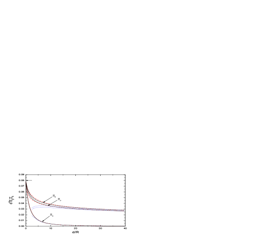
Figure 2: The contributions to the energy shift in the retarded limit due to the three components of the atomic dipole, multiplied by $E_{ji}d^{4}$. Solid lines represent the results of exact numerical integration of Eqs. (LABEL:FinalC1)–(LABEL:FinalC3) in the limit $E_{ji}\rightarrow\infty$, whereas the dashed (red) lines represent the approximations (III.1.4)–(33). For large $d$ the asymptotic behaviour is dominated by the lowest $m$ terms in the sums, given by (36)–(38) and shown as dotted (blue) lines. The arrow on the vertical axis indicates the exact value in the limit $d\rightarrow 0$, Eq. (35).

In the limit of the distance $d=\rho-R$ being much smaller than the radius $R$ of the wire, the above approximations yield

$$\Xi_{\rho}\approx\Xi_{\phi}\approx\Xi_{z}\approx\frac{1}{4\pi d^{4}}\frac{1}{E_{ji}}\;,$$ (35)

which agrees with the retarded energy shift of an atom in front of a perfectly reflecting plane mirror, as calculated by Casimir and Polder casimir . This is what one would expect because an atom that is very close to the surface is not susceptible to the curvature of the surface.

III.1.5 $\lambda_{ji}\ll R\ll d$

In this case we again start by taking the limit $E_{ji}\rightarrow\infty$ in Eqs. (LABEL:FinalC1)–(LABEL:FinalC3), which gives a leading order contribution proportional to $1/E_{ji}$. For distances $d$ much larger than the wire radius $R$ the dominant contribution to the sum then comes from the summands with the lowest $m$, so that we need consider only those,

$$\Xi_{\rho}\approx\frac{1}{2\pi E_{ji}}\left\{\int_{0}^{\infty}\mathrm{d}k\,k^{3}\frac{I_{0}(kR)}{K_{0}(kR)}[K_{1}(k\rho)]^{2}\right.$$ (36)

$$\hskip 42.67912pt\left.-2\int_{0}^{\infty}\mathrm{d}k\,\frac{k}{\rho^{2}}\frac{I_{1}^{\prime}(kR)}{K_{1}^{\prime}(kR)}[K_{1}(k\rho)]^{2}\right\},$$

$$\Xi_{\phi}\approx\frac{1}{2\pi E_{ji}}\left\{\int_{0}^{\infty}\mathrm{d}k\,k\!\left(k^{2}+\frac{2}{\rho^{2}}\right)\!\frac{I_{1}(kR)}{K_{1}(kR)}[K_{1}(k\rho)]^{2}\right.$$ (37)

$$\hskip 42.67912pt\left.-2\int_{0}^{\infty}\mathrm{d}k\,k^{3}\frac{I_{1}^{\prime}(kR)}{K_{1}^{\prime}(kR)}[K_{1}^{\prime}(k\rho)]^{2}\right\},$$

$$\Xi_{z}\approx\frac{1}{\pi E_{ji}}\int_{0}^{\infty}\mathrm{d}k\,k^{3}\frac{I_{0}(kR)}{K_{0}(kR)}[K_{0}(k\rho)]^{2}\;.$$ (38)

The dotted lines in Fig. 2 show that these are indeed good approximations for large $d/R$. Their leading-order behaviour is

$$\Xi_{\rho}\propto\frac{1}{E_{ji}}\frac{1}{d^{4}\ln d},\;\;\Xi_{\phi} \!\!\propto \!\!\frac{1}{E_{ji}}\frac{R^{2}}{d^{6}},\;\;\Xi_{z}\propto\frac{1}{E_{ji}}\frac{1}{d^{4}\ln d}\;,$$

which is in full agreement with the asymptotic results by Barash , even though those are for a metallic wire characterized by a plasma frequency. This is because in the retarded limit the interaction between the atom and the surface depends, to leading order, only on the static polarizability.

As in the electrostatic case, the contributions due to the $\rho$ and $z$ components of the atomic dipole fall off less rapidly than the $\phi$ contribution. We also note that, just as in the non-retarded case, the series in powers of $1/\ln d$ converge too slowly to be of any practical use, so that estimates must be made with Eqs. (36)–(38).

III.1.6 $R\ll\lambda_{ji}\ll d$

As in the non-retarded cases, the limit of vanishing radius ($R\rightarrow 0$) and the retarded limit ($E_{ji}\rightarrow\infty$) commute, and we recover the results of the previous section, Eqs. (36)–(38). This is another manifestation of the fact that the criterion of whether the interaction is retarded depends solely on the distance $d$ between an atom and the surface of the wire, and that the relative size of geometrical features and the wavelength $\lambda_{ji}$ is irrelevant. This means in particular that there are no resonance effects for $\lambda_{ji}$ coïnciding with the wire radius $R$.

III.2 Numerical results

For intermediate parameter ranges one has to evaluate Eqs. (LABEL:FinalC1)–(LABEL:FinalC3) numerically. This is straightforward, and one can employ standard software packages like Mathematica or Maple. The numerical convergence of Eqs. (LABEL:FinalC1)–(LABEL:FinalC3) is very good, although more terms are needed for small distances $d$ than for large distances. Figs. 3–5 show the contributions by the $\rho$, $\phi$, and $z$ components of the atomic dipole to the energy shift (15) for various values of the typical transition frequency $E_{ji}$ in the atom. We give the distance $d$ and the transition wavelength $1/E_{ji}$ in units of the wire radius $R$. For plotting we have factored out of $\Xi_{\rho,\phi,z}$ the asymptotic functional dependence of the shift in front of a plane mirror, Eq. (35).

Figure 3: The contribution (LABEL:FinalC1) to the energy shift (15) due to the $\rho$ component of the dipole for various typical transition frequencies $E_{ji}$. The dashed line is this contribution in the retarded limit $E_{ji}\rightarrow\infty$.

Figure 4: The contribution (LABEL:FinalC2) to the energy shift (15) due to the $\phi$ component of the dipole for various typical transition frequencies $E_{ji}$. The dashed line is this contribution in the retarded limit $E_{ji}\rightarrow\infty$.

Figure 5: The contribution (LABEL:FinalC3) to the energy shift (15) due to the $z$ component of the dipole for various typical transition frequencies $E_{ji}$. The dashed line is this contribution in the retarded limit $E_{ji}\rightarrow\infty$.

In Fig. 6 we show how these contributions look when we choose the wavelengths $1/E_{ji}$ of a typical internal transition as a lengthscale and plot the contributions to the energy shift for various wire radii $R$. The larger the value of $R$ the more terms are required in the numerical series.

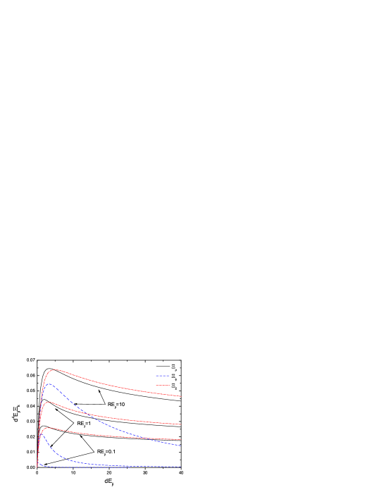
Figure 6: The contributions (LABEL:FinalC1)–(LABEL:FinalC3) to the energy shift (15) due to the $\rho$, $\phi$, and $z$ components of the dipole for various radii $R$ of the wire.

IV ENERGY SHIFT NEAR A PERFECTLY REFLECTING SEMI-INFINITE HALFPLANE

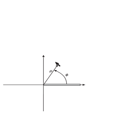
Figure 7: An atomic dipole in the vicinity of a perfectly reflecting semi-infinite halfplane. The normal modes $\mathbf{F}_{\lambda}^{(\sigma)}(\mathbf{x})$ in this geometry are given by Eqs. (39) and (40).

Next we wish to calculate the energy shift of an atom in the vicinity of a perfectly reflecting halfplane, as illustrated by Fig. 7.

The procedure of obtaining the normal modes of the vector potential is analogous to that described in Section III. The scalar solution of the Helmholtz equation (4) in the cylindrical coordinates that is best suited to applying boundary conditions on the surface of the halfplane is given by

$$\Phi(\mathbf{x})=\bigg{[}\frac{\alpha}{\sqrt{\pi}}\sin\left(\frac{m}{2}\phi\right)+\frac{\beta}{\sqrt{\pi}}\cos\left(\frac{m}{2}\phi\right)\bigg{]}J_{m/2}(k\rho)\;\frac{e^{{\rm i}\kappa z}}{\sqrt{2\pi}}\;,$$

where $J_{m/2}(k\rho)$, with $m=0,1,2,\ldots$, are the regular solutions of Bessel’s equation, and the separation constants satisfy $\omega^{2}=k^{2}+\kappa^{2}$. We must have $m\geq 0$, as otherwise the solutions are not linearly independent. Note that half-integer indices arise because the angle $\phi$ is restricted to the interval $[0,2\pi]$, so that the usual argument of single-valuedness of $e^{{\rm i}m\phi}$ cannot be evoked.

In order to obtain two linearly independent vector solutions we again apply Eqs.  (8) and (9), and impose the boundary conditions for a perfectly reflecting halfplane, $E_{\rho}=0=E_{z}$ and $B_{\phi}=0$ for $\phi=0$ and $\phi=2\pi$. In this way we find for the mode functions

$$\mathbf{F}_{\lambda}^{(1)}(\mathbf{r}) \!\!= \!\!-\frac{1}{\sqrt{2}\pi}\bigg{[}\frac{m}{2k\rho}\sin\left(\frac{m}{2}\phi\right)J_{m/2}(k\rho)\;\hat{\mathbf{e}}_{\rho}$$ (39)

$$\!\!+ \!\!\cos\left(\frac{m}{2}\phi\right)J^{\prime}_{m/2}(k\rho)\;\hat{\mathbf{e}}_{\phi}\bigg{]}e^{{\rm i}\kappa z},$$

$$\mathbf{F}_{\lambda}^{(2)}(\mathbf{r}) \!\!= \!\!\frac{1}{\sqrt{2}\pi}\bigg{[}\frac{i\kappa}{\omega}\sin\left(\frac{m}{2}\phi\right)J^{\prime}_{m/2}(k\rho)\;\hat{\mathbf{e}}_{\rho}$$ (40)

$$\!\!+ \!\!\frac{i\kappa m}{2k\rho\omega}\cos\left(\frac{m}{2}\phi\right)J_{m/2}(k\rho)\;\hat{\mathbf{e}}_{\phi}$$

$$\!\!+ \!\!\frac{k}{\omega}\sin\left(\frac{m}{2}\phi\right)J_{m/2}(k\rho)\;\hat{\mathbf{e}}_{z}\bigg{]}e^{{\rm i}\kappa z},$$

where the composite index stands for $\lambda=\{k,m,\kappa\}$. For $m>0$ these mode functions satisfy the normalization condition (11), but the first polarization has an additional mode with $m=0$ for which Eq. (39) must be multiplied by an additional factor $1/\sqrt{2}$ for it to be normalized correctly according to (11),

$$\mathbf{F}_{m=0}^{(1)}(\mathbf{r})=-\frac{1}{2\pi}J^{\prime}_{0}(k\rho)\;\hat{\mathbf{e}}_{\phi}\;e^{{\rm i}\kappa z}\;.$$ (41)

Substituting the mode functions (39)-(41) into Eq. (6) and renormalizing the energy shift by subtracting the free-space contribution in the same way as this was done in Eqs. (16)-(18), we obtain an energy shift of the form (15) with

$$\Xi_{\rho} \!\!= \!\!\frac{2}{\pi}\int_{0}^{\infty}\mathrm{d}k\;k\int_{0}^{\infty}\mathrm{d}\kappa\;\frac{\omega}{E_{ji}+\omega}\left\{\left(\frac{1}{k\rho}\right)^{2}\sum_{m=1}^{\infty}\left[\left(\frac{m}{2}\right)^{2}\sin^{2}\left(\frac{m}{2}\phi\right)J^{2}_{m/2}(k\rho)-m^{2}J^{2}_{m}(k\rho)\right]\right.$$ (42)

$$\!\!+ \!\!\left.\left(\frac{\kappa}{\omega}\right)^{2}\sum_{m=0}^{\infty}\!\>{}^{\prime}\left[\sin^{2}\left(\frac{m}{2}\phi\right)J^{\prime 2}_{m/2}(k\rho)-J^{\prime 2}_{m}(k\rho)\right]\right\},$$

$$\Xi_{\phi} \!\!= \!\!\frac{2}{\pi}\int_{0}^{\infty}\mathrm{d}k\;k\int_{0}^{\infty}\mathrm{d}\kappa\;\frac{\omega}{E_{ji}+\omega}\left\{\sum_{m=0}^{\infty}\!\>{}^{\prime}\left[\cos^{2}\left(\frac{m}{2}\phi\right)J^{\prime 2}_{m/2}(k\rho)-J^{\prime 2}_{m}(k\rho)\right]\right.$$ (43)

$$\!\!+ \!\!\left.\left(\frac{\kappa}{k\rho\omega}\right)^{2}\sum_{m=1}^{\infty}\left[\left(\frac{m}{2}\right)^{2}\cos^{2}\left(\frac{m}{2}\phi\right)J^{2}_{m/2}(k\rho)-m^{2}J^{2}_{m}(k\rho)\right]\right\},$$

$$\Xi_{z} \!\!= \!\!\frac{2}{\pi}\int_{0}^{\infty}\mathrm{d}k\;k\int_{0}^{\infty}\mathrm{d}\kappa\;\frac{\omega}{E_{ji}+\omega}\left\{\left(\frac{k}{\omega}\right)^{2}\sum_{m=0}^{\infty}\!\>{}^{\prime}\left[\sin^{2}\left(\frac{m}{2}\phi\right)J^{2}_{m/2}(k\rho)-J^{2}_{m}(k\rho)\right]\right\},$$ (44)

where the primes on the sums indicate that the $m=0$ terms are weighted by an additional factor of 1/2. In order to simplify these expressions, the sums over the Bessel functions need to be evaluated. Recently, similar summations have been carried out Farina2 ; Farina1 , but the results obtained do not include our particular case of sums involving Bessel functions of the half-integer order.

We proceed along the following lines. First, we split each sum into two, one over Bessel functions of integer orders, and the other over half-integer orders. For the first we can apply the standard summation formula (AS, , 9.1.79)

$$\sum_{m=0}^{\infty}\!{}^{\prime}\;\cos 2m\phi\;J_{m}^{2}(z)=\frac{1}{2}J_{0}(2z\sin\phi)\;,$$ (45)

and we choose to represent the right-hand side in terms of an integral (AS, , 9.1.24)

$$\frac{1}{2}J_{0}(2z\sin\phi)=\frac{1}{\pi}\int_{1}^{\infty}\mathrm{d}t\;\frac{\sin(2zt\sin\phi)}{\sqrt{t^{2}-1}}\;.$$ (46)

For the half-integer sum we use a summation formula of (Prudnikov, , 5.7.17.(11.)), which in our case gives

$$\sum_{m=0}^{\infty}\cos(2m+1)\phi\;J_{m+\frac{1}{2}}^{2}(z)=\frac{1}{\pi}\int_{1}^{1/\sin\phi}\!\!\mathrm{d}t\;\frac{\sin(2zt\sin\phi)}{\sqrt{t^{2}-1}}\;.$$ (47)

We note that, if we use the integral representation (46), the sums over integer and over half-integer Bessel functions are very similar; the only difference is the upper limit of the $t$ integral in (46) and (47). As these $t$ integrals and their derivatives will arise repeatedly, we define the following auxiliary functions:

$$F(z,\phi)\equiv\int_{1}^{1/\sin\phi}\!\!\mathrm{d}t\;\frac{\sin(2zt\sin\phi)}{\sqrt{t^{2}-1}}\;,$$ (48)

$$G(z,\phi)\equiv\int_{1}^{\infty}\mathrm{d}t\;\frac{\sin(2zt\sin\phi)}{\sqrt{t^{2}-1}}\;.$$ (49)

Further we note that the $\kappa$ integrals in Eqs. (42)-(44) suffer from the same convergence problems as already discussed in Section III. We avoid these by introducing polar coordinates with ${k=\omega\sin\alpha}$ and ${\kappa=\omega\cos\alpha}$. At the same time we parametrize the denominator arising from perturbation theory by

$$\frac{1}{E_{ji}+\omega}=\int_{0}^{\infty}\mathrm{d}x\;e^{-(E_{ji}+\omega)x}\;,$$ (50)

with $E_{ji}+\omega=E_{ji}+\sqrt{k^{2}+\kappa^{2}}\geq 0$. Then Eqs. (42)-(44) become

$$\Xi_{\rho} \!\!= \!\!\frac{2}{\pi}\int_{0}^{\infty}\mathrm{d}x\;e^{-E_{ji}x}\int_{0}^{\infty}\mathrm{d}\omega\;\omega^{3}e^{-\omega x}\int_{0}^{\pi/2}\mathrm{d}\alpha\sin\alpha$$ (51)

$$\hskip 14.22636pt\times\left\{\sigma_{1}(\omega\rho\sin\alpha)+\sigma_{3}(\omega\rho\sin\alpha)\cos^{2}\alpha\right\},$$

$$\Xi_{\phi} \!\!= \!\!\frac{2}{\pi}\int_{0}^{\infty}\mathrm{d}x\;e^{-E_{ji}x}\int_{0}^{\infty}\mathrm{d}\omega\;\omega^{3}e^{-\omega x}\int_{0}^{\pi/2}\mathrm{d}\alpha\sin\alpha$$ (52)

$$\hskip 14.22636pt\times\left\{\sigma_{2}(\omega\rho\sin\alpha)\cos^{2}\alpha+\sigma_{4}(\omega\rho\sin\alpha)\right\},$$

$$\Xi_{z} \!\!= \!\!\frac{2}{\pi}\int_{0}^{\infty}\mathrm{d}x\;e^{-E_{ji}x}\int_{0}^{\infty}\mathrm{d}\omega\;\omega^{3}e^{-\omega x}\int_{0}^{\pi/2}\mathrm{d}\alpha\sin\alpha$$ (53)

$$\hskip 14.22636pt\times\left\{\sigma_{5}(\omega\rho\sin\alpha)\sin^{2}\alpha\right\}.$$

The sums $\sigma_{i}(z)$ appearing in these expressions can be calculated by using Eqs. (45)–(49) and standard derivative formulae for Bessel functions (AS, , 9.1.27); we obtain in terms of (48) and (49):

$$\left[\begin{array}[]{c}\sigma_{1}(z)\\ \sigma_{2}(z)\end{array}\right] \!\!= \!\!\frac{1}{z^{2}}\sum_{m=1}^{\infty}\left\{\left(\frac{m}{2}\right)^{2}\left[\begin{array}[]{c}\sin^{2}\left(m\phi/2\right)\\ \cos^{2}\left(m\phi/2\right)\end{array}\right]J^{2}_{m/2}(z)-m^{2}J^{2}_{m}(z)\right\}$$ (58)

$$\!\!= \!\!\frac{1}{8\pi z^{2}}\left[\pm\frac{\partial^{2}G(z,\phi)}{\partial\phi^{2}}+\frac{\partial^{2}G(z,\phi)}{\partial\phi^{2}}\bigg{|}_{\phi=0}\pm\frac{\partial^{2}F(z,\phi)}{\partial\phi^{2}}-\frac{\partial^{2}F(z,\phi)}{\partial\phi^{2}}\bigg{|}_{\phi=0}\right],$$ (59)

$$\left[\begin{array}[]{c}\sigma_{3}(z)\\ \sigma_{4}(z)\end{array}\right] \!\!= \!\!\sum_{m=0}^{\infty}\!\!\;{}^{\prime}\left\{\left[\begin{array}[]{c}\sin^{2}\left(m\phi/2\right)\\ \cos^{2}\left(m\phi/2\right)\end{array}\right]J^{\prime 2}_{m/2}(z)-J^{\prime 2}_{m}(z)\right\}$$ (64)

$$\!\!= \!\!-\left[\begin{array}[]{c}\sigma_{1}(z)\\ \sigma_{2}(z)\end{array}\right]+\frac{1}{2\pi}\big{[}F(z,0)-G(z,0)\big{]}\mp\frac{\cos 2\phi}{2\pi}\big{[}F(z,\phi)+G(z,\phi)\big{]}+\frac{\cos 2z}{2\pi z}(1\mp\cos\phi)\;,$$ (67)

$$\sigma_{5}(z) \!\!= \!\!\sum_{m=0}^{\infty}\!\!\;{}^{\prime}\left\{\sin^{2}\left(m\phi/2\right)J^{2}_{m/2}(z)-J^{2}_{m}(z)\right\}$$ (68)

$$\!\!= \!\!\frac{1}{2\pi}\big{[}F(z,0)-F(z,\phi)-G(z,\phi)-G(z,0)\big{]}\;.$$

We now carry out the various integrations in the following order. First we evaluate the $\alpha$ integrals, which all give Bessel functions $J_{1}$ or $J_{0}$ (GR, , 3.715(10),(14)). Next we carry out the integrations over $\omega$, which involve integrals of the type (GR, , 6.611(1.))

$$\int_{0}^{\infty}\mathrm{d}z\;e^{-az}\,J_{\nu}(bz)=\frac{b^{-\nu}\left(\sqrt{a^{2}+b^{2}}-a\right)^{\nu}}{\sqrt{a^{2}+b^{2}}}\;.$$

Finally, we calculate the $t$ integrals that came in through the auxiliary functions $F$ and $G$, Eqs. (48) and (49). These are all elementary. At the very end we calculate the $\phi$ derivatives of Eq. (59) and take the limit $\phi\rightarrow 0$ in the appropriate terms. The end results then still contain the parameter integral (50) over $x$, which we now scale by substituting $x=2\rho\eta$. Then the final results read

$$\Xi_{\rho} \!\!= \!\!\frac{1}{16\pi\rho^{3}}\int_{0}^{\infty}\mathrm{d}\eta\;e^{-2\rho E_{ji}\eta}\left\{\frac{3\eta^{4}+6\eta^{2}+4}{\eta^{4}(1+\eta^{2})^{3/2}}-\frac{4}{\eta^{4}}+\frac{4}{(\eta^{2}+\sin^{2}\phi)^{3}}\left[(2\eta^{2}+1)\sin^{2}\phi-\eta^{2}\right]\right.$$ (69)

$$\!\!+ \!\!\left.\frac{\cos\phi}{(1+\eta^{2})^{3/2}(\eta^{2}+\sin^{2}\phi)^{3}}\left[(2+\eta^{2})\sin^{4}\phi+2\sin^{2}\phi(3\eta^{4}+6\eta^{2}+2)-\eta^{2}(3\eta^{4}+6\eta^{2}+4)\right]\right\},$$

$$\Xi_{\phi} \!\!= \!\!\frac{1}{16\pi\rho^{3}}\int_{0}^{\infty}\mathrm{d}\eta\;e^{-2\rho E_{ji}\eta}\left\{\frac{3\eta^{6}+6\eta^{4}+10\eta^{2}+4}{\eta^{4}(1+\eta^{2})^{5/2}}-\frac{4}{\eta^{4}}+\frac{4}{(\eta^{2}+\sin^{2}\phi)^{3}}\left[(1-2\eta^{2})\sin^{2}\phi+\eta^{2}\right]\right.$$

$$\!\!+ \!\!\left.\frac{\cos\phi}{(1+\eta^{2})^{5/2}(\eta^{2}+\sin^{2}\phi)^{3}}\left[(2-2\eta^{2}-\eta^{4})\sin^{4}\phi+2\sin^{2}\phi(2+2\eta^{2}-6\eta^{4}-3\eta^{6})+\eta^{2}(3\eta^{6}+6\eta^{4}+10\eta^{2}+4)\right]\right\},$$

$$\Xi_{z} \!\!= \!\!\frac{1}{16\pi\rho^{3}}\int_{0}^{\infty}\mathrm{d}\eta\;e^{-2\rho E_{ji}\eta}\left\{\frac{9\eta^{4}+10\eta^{2}+4}{\eta^{4}(1+\eta^{2})^{5/2}}-\frac{4}{\eta^{4}}+4\frac{\sin^{2}\phi-\eta^{2}}{(\eta^{2}+\sin^{2}\phi)^{3}}\right.$$ (71)

$$\!\!- \!\!\left.\frac{\cos\phi}{(1+\eta^{2})^{5/2}(\eta^{2}+\sin^{2}\phi)^{3}}\left[(\eta^{2}-2)\sin^{4}\phi+2(\eta^{4}-4\eta^{2}-2)\sin^{2}\phi+\eta^{2}(9\eta^{4}+10\eta^{2}+4)\right]\right\}.$$

Inserted into Eq. (15) the Eqs. (69)–(71) give the final result for the energy shift of an atom near a perfectly reflecting halfplane. Some of the integrations over the auxiliary variable $\eta$ could in principle be carried out, but those would yield complicated hypergeometric functions. Thus it is preferable to have the result in the form of an integral over elementary functions. It converges quickly and can therefore be very easily evaluated numerically by using standard software packages. In addition, we shall go on to determine asymptotic expressions in the non-retarded and retarded regimes.

IV.1 Asymptotic regimes.

IV.1.1 Plane-mirror limit

In the limit of the polar angle $\phi$ being very small, the atom is very close to the halfplane but far away from the edge, so that the energy shift should be the same as for an atom in front of a plane, infinitely extended mirror. The component of the atomic dipole that is normal to the surface should then give the contribution listed in Eq. (29) to the shift, and the parallel components should contribute that shown in Eq. (30). As the distance $d$ of the atom from the halfplane is $\rho\sin\phi$, we take Eqs. (69)–(71) and scale $\eta\rightarrow\eta\sin\phi$, so as to get an exponential with the same argument as in Eqs. (29) and (30). If we subsequently take the limit $\phi\rightarrow 0$, we recover Eqs. (29) and (30), as expected. Note, however, that the geometry is different from the cylindrical case: the $\phi$ component of the atomic dipole is now normal to the surface and its contribution $\Xi_{\phi}$ to the energy shift is given by (29), and the $\rho$ and $z$ components are parallel so that $\Xi_{\rho}$ and $\Xi_{z}$ are given by (30).

IV.1.2 Non-retarded regime

If $\rho E_{ji}\ll 1$ then the atom is very close to the halfplane, compared to the wavelength of a typical internal transition. This means that the interaction of the atom and the surface is instantaneous, as the atom evolves on a much longer timescale. In this case field quantization is not necessary, and only Coulomb interactions between the atom and the halfplane need to be considered, as was done in Ref. nonret , where we derived

$$\Xi_{\rho} \!\!= \!\!\frac{5}{48\pi\rho^{3}}+\frac{\cos\phi}{16\pi\rho^{3}\sin^{2}\phi}+\frac{(\pi-\phi)(1+\sin^{2}\phi)}{16\pi\rho^{3}\sin^{3}\phi}$$

$$\Xi_{\phi} \!\!= \!\!-\frac{1}{48\pi\rho^{3}}+\frac{\cos\phi}{8\pi\rho^{3}\sin^{2}\phi}+\frac{(\pi-\phi)(1+\cos^{2}\phi)}{16\pi\rho^{3}\sin^{3}\phi}$$

$$\Xi_{z} \!\!= \!\!\frac{1}{24\pi\rho^{3}}+\frac{\cos\phi}{16\pi\rho^{3}\sin^{2}\phi}+\frac{\pi-\phi}{16\pi\rho^{3}\sin^{3}\phi}\;.$$

Taking the limit $E_{ji}\rightarrow 0$ in Eqs. (69)–(71) we recover these results, which is an important consistency check on our present calculation.

IV.1.3 Retarded regime

In the opposite limit of the atom being far away from the halfplane, we need to distinguish whether the atom is located beyond the edge of the halfplane or not. If it is, i.e. for $\pi/2<\phi<\pi$ the distance of the atom to the halfplane is its distance to the edge, namely $\rho$, so that the condition for the interaction to be fully retarded is $\rho E_{ji}\gg 1$. If, on the other hand, $0<\phi<\pi/2$ then the distance to the halfplane is $\rho\sin\phi$, and consequently the criterion for full retardation is $\rho\sin\phi E_{ji}\gg 1$, cf. Fig. 7.

Taking the limit $E_{ji}\rightarrow\infty$ in the integrals (69)-(71) is straightforward, since, according to Watson’s lemma Bender , the integral is then dominated by contributions from the vicinity of $\eta=0^{+}$, so that one just needs to factor out the exponential and expand the rest of the integrand in the curly brackets in a Taylor series about this point. The leading terms of these Taylor expansions turn out to be constants with respect to $\eta$ in each case. Thus in the retarded limit we obtain

$$\Xi_{\rho} \!\!= \!\!\frac{1}{64\pi\rho^{4}E_{ji}}\left[3+\frac{1}{\sin^{4}(\phi/2)}+\frac{2}{\sin^{2}(\phi/2)}\right]$$ (72)

$$\Xi_{\phi} \!\!= \!\!\frac{1}{64\pi\rho^{4}E_{ji}}\left[-3+\frac{1}{\sin^{4}(\phi/2)}+\frac{2}{\sin^{2}(\phi/2)}\right]$$ (73)

$$\Xi_{z} \!\!= \!\!\frac{1}{64\pi\rho^{4}E_{ji}}\left[3+\frac{1}{\sin^{4}(\phi/2)}+\frac{2}{\sin^{2}(\phi/2)}\right],$$ (74)

which, for the case of isotropic polarizability, is in agreement with the result of Ref. Brevik . In the light of our comments above, we emphasize again that these results are only valid when the distance of the atom from the halfplane exceeds several wavelengths $\lambda_{ji}$. This means that for small angles $\phi$ one needs to revert to the plane-mirror limit discussed in Section IV.1.1 above, because in the region $0<\phi<\pi/2$ Eqs. (72)–(74) apply only if $\sin\phi\gg\lambda_{ji}/\rho$. However, taking the limit $\rho\rightarrow\infty$ together with $\phi\rightarrow 0$ while keeping $\rho\sin\phi=d$ fixed is legitimate, and reproduces the well-known Casimir-Polder result casimir for the retarded interaction between an atom and a plane mirror, Eq. (35).

Taking the limit $\phi\rightarrow\pi$ in Eqs. (72)–(74) shows that for an atomic dipole that is polarized azimuthally the interaction vanishes when the atom is located exactly above the edge of the halfplane. This conclusion actually holds not just in the retarded regime, but generally for any distance, as Eq. (LABEL:Final2) also vanishes in the limit $\phi\rightarrow\pi$. Purely from symmetry one would expect there to be no azimuthal component to the Casimir-Polder force directly above the edge, but the fact that there is no radially directed force either is surprising.

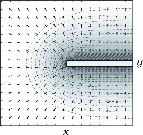
Figure 8: Direction of the retarded Casimir-Polder force acting on the atom with isotropic polarizability. Note from Eqn. (LABEL:Final2) that an atom that is polarized azimuthally does not experience any force when it is located exactly above the edge of the halfplane.

Since we have worked in the cylindrical coordinates, the direction of the unit vectors $\hat{\mathbf{e}}_{\rho}$ and $\hat{\mathbf{e}}_{\phi}$ depends on the position coordinates $\rho$ and $\phi$. In this context it is curious that, in the retarded limit, all three components of the atomic dipole contribute to the energy shift with exactly the same angular dependence.

V summary

We have calculated the energy shift in a neutral atom caused by the presence at arbitrary distance of perfectly reflecting microstructures of two different geometries. For an atom at a distance $d=\rho-R$ from the perfectly reflecting cylindrical wire of radius $R$ we have found an exact expression for the interaction energy, Eq. (15) with Eqs. (LABEL:FinalC1)-(LABEL:FinalC3). As these integrals and sums are in general quite complicated, we have analysed various important limiting cases. The limit of the distance $d$ being small on the scale of the wavelength $\lambda_{ji}$ of a typical atomic transition requires only electrostatic forces to be considered, which was done in detail in Ref. nonret . The case of purely retarded interactions, which occur when the distance $d$ is much larger than $\lambda_{ji}$, has been analysed in Sections III.1.4–6. For a small wire radius the three contributions to the energy shift are well approximated by Eqs. (36)–(38), and for a large wire radius by Eqs. (III.1.4)–(33).

In the case of an atom close to a perfectly reflecting halfplane the exact analytic analysis can be pushed a little bit further than in the cylindrical case. We have managed to find an exact formula for the energy shift in terms of a simple, rapidly converging integral over elementary functions, Eqs. (69)-(71), so that they are very easy to study numerically. Nevertheless, we have also derived asymptotic formulae, which agree with previous calculations.

The totality of our results can be used to reliably estimate the energy shift in an atom close to a variety of common microstructures that consist of a ledge and possibly an electroplated top layer of higher reflectivity. We have determined the energy shifts for the complete range of distances, which is very important for practical applications as in many modern experiments the distance of the atom is neither much larger nor much smaller than the typical wavelength of an atomic transition, but commensurate.

References

• (1) C. Eberlein and R. Zietal, Phys. Rev. A 75, 032516(2007).
• (2) H.B.G. Casimir, D. Polder, Phys. Rev. 73, 360 (1948)
• (3) Yu.S. Barash, A.A. Kyasov, Sov. Phys. JETP 68, 1(1989).
• (4) Ya.B. Zel’dovich, Zh. Eksp. Theor. Fiz. 5, 22(1935).
• (5) V.M. Nabutovskii, V.R. Belosludov, A.M. Korotkikh, Sov. Phys. JETP 50, 2 (1979).
• (6) A.M. Marvin, F. Toigo, Phys. Rev. A 25, 782(1982).
• (7) M.J. Mehl, W.L. Schaich, Phys. Rev. A 16, 921(1977).
• (8) M.J. Mehl, W.L. Schaich, Phys. Rev. A 21, 1177(1980).
• (9) D. Langbein, Theory of Van der Waals attraction (Springer, Berlin, 1974).
• (10) A.M. Marvin, F. Toigo, Phys. Rev. A 25, 803(1982).
• (11) D. P. Fussell, R. C. McPhedran, C. Martijn de Sterke, Phys. Rev. A 71, 013815(2005).
• (12) M. Boustimi, J. Baudon, P. Candori, J. Robert, Phys. Rev. B 65, 155402(2002).
• (13) M. Boustimi, J. Baudon, J. Robert, Phys. Rev. B 67, 045407(2003).
• (14) E. V. Blagov, G. L. Klimchitskaya, V. M. Mostepanenko, Phys. Rev. B 71, 235401(2005).
• (15) I. Brevik, M. Lygren, V.N. Marachewsky Ann. Phys. (NY) 267, 134-142 (1988).
• (16) T.N.C. Mendes, F.S.S. da Rosa, A. Tenorio, C. Farina, J. Phys. A 41, 164029(2008).
• (17) I.S. Gradshteyn and I.M. Ryzhik, Table of Integrals, Series, and Products, edited by A. Jeffrey (Academic Press, London, 1994), 5th ed.
• (18) Handbook of Mathematical Functions, edited by M. Abramowitz and I. Stegun (US GPO, Washington, DC, 1964).
• (19) F.S.S. da Rosa, T.N.C. Mendes, A. Tenorio, C. Farina, Phys. Rev. A 78, 012105 (2008).
• (20) A.P. Prudnikov, Yu.A. Brychkov, O.I. Marichev, Integrals and Series, Volume 2: Special Functions (Gordon and Breach, New York, 1992), 3rd printing with corrections.
• (21) C.M. Bender, S. A. Orszag, Advanced Mathematical Methods for Scientists and Engineers, (Springer, Berlin, 1999).