Phase separation in doped systems with spin-state transitions

Abstract

Spin-state transitions, observed in many transition metal compounds containing Co³⁺ and Fe²⁺, may occur with the change of temperature, pressure, but also with doping, in which case the competition of single-site effects and kinetic energy of doped carriers can favor a change in the spin state. We consider this situation in a simple model, formally resembling that used for manganites in Ref. myPRL, . Based on such a model, we predict the possibility of a jump-like change in the number of Co³⁺ ions undergoing spin-state transition caused by hole doping. A tendency to the electronic phase separation within a wide doping range is demonstrated. Phase diagrams with the regions of phase separation are constructed at different values of the characteristic parameters of the model.

I Introduction

Interplay of different degrees of freedom and different types of ordering is a very important ingredient in determining the properties of strongly correlated electron systems. Especially interesting these effects become in doped systems. Typical for this case is the tendency to phase separation and formation of inhomogeneous states. It can take different forms: formation of isolated polarons or small clusters (modification of a particular ordering by doped charge carriers and the trapping of charge carriers in a distorted region) or particular textures, e.g. stripes. Such phase separation can play a very important role in many phenomena, such as colossal magnetoresistance in manganites dagbook , and probably also in high-Tc superconductors - although their role in the latter is still a matter of hot debate.

The most common and best known case is the doping of antiferromagnetic insulators, with the formation of ferromagnetic droplets (“ferrons”) or charged antiferromagnetic domain walls (stripes) dagbook ; Nag ; Kak . We have recently shown that, similarly, the interplay of kinetic energy of doped holes with the orbital structure can give rise to a novel mechanism of phase separation orbPS1 ; orbPS2 .

A special interesting group of phenomena is met in systems where the respective ions can exist in different multiplet states. Typical examples are the compounds containing Co³⁺ (or sometimes Fe²⁺), which can exist in a low-spin (LS) state with $S$=0 ($t_{2g}^{6}$), intermediate-spin (IS) state $S=1$ ($t_{2g}^{5}e_{g}^{1}$), and high-spin (HS) state ($t_{2g}^{4}e_{g}^{2}$) with $S=2$, see e.g. Ref. Gooden67, . Close proximity in energy of these states can lead to a special type of transition (or crossover): spin-state transition (SST), typical example being LaCoO₃ Gooden67 ; Tokura1 ; Tokura2 ; Korotin . Also spin-state ordering is possible Doumerc ; KhoLow . Thus, these systems, in addition to quite common charge, orbital, and spin degrees of freedom with the possibility of respective orderings, have an “extra dimension”: the possibility of spin-state (or, in other words, multiplet) transitions. Correspondingly, if doping of materials like manganites can cause phase separation due to an interplay of the motion (kinetic energy) of doped holes with the underlying magnetic and orbital structure, in systems with SST like cobaltites one can expect similar phenomena due to an interplay with the spin state of the matrix. The common mechanisms causing the phase separation manifest themselves in the situation when the particular ordering existing in the system hinders the motion of doped holes. In these cases, it may be favorable to locally modify the type of ordering, facilitating the motion of the hole in such distorted region. Thus, holes can hardly move on an antiferromagnetic background, which was noticed already long ago both for the two-band (double exchange) model AndHas ; deGennes and for the single-band (Hubbard) model BulKhom67 ; BulNagKhom . At the same time a hole moves freely on the ferromagnetic background. As a result, ferromagnetic polarons (ferrons) may be formed close to the hole, and the gain in kinetic energy of the latter moving on the ferromagnetic background exceeds the loss of the magnetic energy Nag67 ; Kasuya ; BulNagKhom .

Similarly, certain types of orbital ordering suppress hole motion, and it may be favorable to modify orbital pattern close to a hole, forming orbital polaron and facilitating motion of a hole within it  orbPS1 ; KilKha ; MiKhoSaw . For systems with SST such a role can be played for example by the phenomenon of a spin blockade SpinBlock : if one dopes the material with the Co³⁺ in a low-spin state ($S=0$) by electrons, the ionic state created could be Co²⁺ in a high-spin state ($S=3/2$). In this case, it is evident that it is not possible to interchange the states Co³⁺ LS and Co²⁺ HS by moving only one electron: one would end up in the “wrong” states Co³⁺ and Co²⁺ both in IS states, not in the original states (the hopping of an electron can change the spin of corresponding states only by $\pm 1/2$, whereas the spins of the original states differ by 3/2). As a consequence, an extra electron can only move in a crystal leaving the trace of wrong spin states, which will lead to a confinement and localization of this electron, similar to the case of the usual Hubbard model BulNagKhom .

One can “repair” this by modifying the spin state in the vicinity of a charge carrier (electron or hole), and this will finally again lead to a creation of inhomogeneous states and to phase separation. This phenomenon was actually observed in some cobaltites, e.g. in La_1-xSr_xCoO₃. There are already many indications of phase separation and formation of inhomogeneous states in this system Rivas ; Loshk ; Louca ; Leighton06 ; Leighton07 , but probably the most clear evidence comes from the study of very low doped LaCoO₃. Magnetic measurements Tokura1 have shown that at very low doping ($<1\%$ of Sr) the moment per doped hole (per Sr) is much bigger than that of only a LS Co⁴⁺ with $S=1/2$: instead there exist magnetic impurities with unusually large spin $S=5-10$, which signals that each hole is “dressed” by the magnetic cloud due to the promotion of some of neighboring Co³⁺ ions to a magnetic state. The magnetic scattering, ESR and NMR study of such system Podles08 allowed even determining the size and shape of such magnetic clusters formed around doped holes.

It is possible to use different approaches to describe theoretically the phenomenon of phase separation. First of all, it is the direct numerical investigation dagbook . Or one can assume the formation of spin-state polarons, calculate their energy and check whether and at which conditions the formation of such polarons can be energetically favorable. But the most direct way, by which one usually starts, is first to assume the existence of a homogeneous state and to check for its stability against phase separation. This was the route taken earlier by us for the double exchange model KaKhoMo , for the situation close to a charge ordering KaKuKh01 , for two-component model of manganites myPRL ; myPRB , or for orbital ordering orbPS1 . If the homogeneous state turns out to be unstable, then at the second step one can investigate particular types of inhomogeneous states, which can be formed. In the present paper, we follow this route for the doped systems with SST.

II Spin states of cobalt ions

Let us list the possible spin states of Co³⁺ and Co⁴⁺ ions in a CoO₆ octahedron, which is a main building block of perovskite-like Co-based compounds (we will consider below the hole-doped cobaltites, nominally containing Co³⁺ and Co⁴⁺). The electron configuration of Co³⁺ ion is $3d^{6}$. It is well known that in the crystal field of cubic symmetry, a $d$-level with the 5-fold orbital degeneracy is split into a doubly degenerate $e_{g}$ level and a triply degenerate $t_{2g}$ level. In the octahedral coordination, the $t_{2g}$ level lies below the $e_{g}$ level. So, a Co³⁺ ion can have three low-energy spin states: low-spin (LS), intermediate-spin (IS), and high-spin (HS) states.

In the LS state ($S=0$), all $t_{2g}$ states are occupied and the $e_{g}$ level is empty. In the IS state ($S=1$), there are five electrons at the $t_{2g}$ level and one $e_{g}$ electron. In the HS state ($S=2$), we have four $t_{2g}$ and two $e_{g}$ electrons. The corresponding energies of these states are $E_{LS}^{(3+)}=E_{0}$, $E_{IS}^{(3+)}=E_{0}+\Delta-J_{H}$, and $E_{HS}^{(3+)}=E_{0}+2\Delta-4J_{H}$, where $\Delta$ is the energy splitting between $t_{2g}$ and $e_{g}$ levels and $J_{H}$ is the Hund’s rule coupling constant. For the Co⁴⁺ ion ($3d^{5}$), there are three similar low-lying spin states, corresponding to different distributions of five electrons between $t_{2g}$ and $e_{g}$ levels. In the LS state ($S=1/2$), there are five electrons at the $t_{2g}$ level and no $e_{g}$ electrons. In the IS state ($S=3/2$), we have four $t_{2g}$ electrons and one $e_{g}$ electron. In the HS state ($S=5/2$), the numbers of $t_{2g}$ and $e_{g}$ electrons are equal to three and two, respectively. The corresponding energies of these states for the Co⁴⁺ ion are $E_{LS}^{(4+)}=E_{1}$, $E_{IS}^{(4+)}=E_{1}+\Delta-2J_{H}$, and $E_{HS}^{(4+)}=E_{1}+2\Delta-6J_{H}$. Here, we introduced $E_{0}$ and $E_{1}$ as some reference energy values for Co³⁺ and Co⁴⁺, respectively. As we shall demonstrate below, the results do not depend much on the specific choice of $E_{0}$ and $E_{1}$. All aforementioned configurations of Co ions and their energies are summarized in Table 1.

Table 1: (Color online) Possible electron configurations of Co ions and their energies.

The type of the ground state for a separate Co³⁺ or Co⁴⁺ ion depends on the relationship between $\Delta$ and $J_{H}$. It can be easily seen that at $\Delta>3J_{H}$, the LS is the ground state both for Co³⁺ and Co⁴⁺. At $2J_{H}<\Delta<3J_{H}$, Co³⁺ still has the LS ground state, whereas for Co⁴⁺ the HS is more favorable. Eventually, at $\Delta<2J_{H}$, the HS state is the lowest in energy for both ions. Hence, for isolated cobalt ions, the IS ground state does not appear.

The situation becomes more complicated if there exists a charge transfer between cobalt ions. First, note that the hopping integrals between the $t_{2g}$ states in cobaltites are as a rule much smaller than for the $e_{g}$ states. In the treatment below, we ignore the $t_{2g}-t_{2g}$ hopping and take into account only the hopping of $e_{g}$ electrons. The inclusion of $t_{2g}-t_{2g}$ hoppings will not modify qualitative results, introducing only minor numerical changes. Second, the states with the number of electrons per ion larger than six are unfavorable due to the strong on-site Coulomb repulsion. Third, the transitions of electrons between the lattice sites corresponding to the changes of spin by more than one half are strongly suppressed since they involve the simultaneous change of a state for two or more electrons.

As a result, in doped cobaltites there remain only two most probable hopping processes: (i) the transitions of electrons between the IS Co³⁺ and LS Co⁴⁺ and (ii) transitions between the HS Co³⁺ and IS Co⁴⁺. The corresponding configurations are illustrated in Table 1. Thus, to facilitate the kinetic energy gain due to the electron transfer, one can create a ground state with intermediate spins. Such a situation can arise if in the ground state for isolated ions, we have either LS Co⁴⁺ or HS Co³⁺. The former case corresponds to $\Delta>3J_{H}$ when some of LS Co³⁺ can be promoted to the IS state. In the latter case corresponding to $\Delta<2J_{H}$, some HS Co⁴⁺ are promoted to the IS state. In the intermediate situation, $2J_{H}<\Delta<3J_{H}$, the electron transfer can occur if we promote both ions, Co³⁺ and Co⁴⁺, to some excited states. Such double excitations seem to be less probable. Below, we first discuss the most realistic case $\Delta>3J_{H}$ at different doping levels with a special emphasis on the possibility of phase separation. Then, we perform the similar study for $\Delta<2J_{H}$. After that, we construct the phase diagram of the system at $\Delta/J_{H}-$doping plane.

Actually, $\Delta$, or rather $\Delta/t$, regularly depends on the rare earth radius $r_{A}$ in the series of RCoO₃ perovskites and increases with decreasing $r_{A}$.

III Charge transfer effects and spin-state transitions: The case of LS-LS ground state for isolated ions

Let us first discuss the situation corresponding to doped perovskite cobaltites, where Co³⁺ and Co⁴⁺ ions occupy the sites of a simple cubic lattice. The relative number of Co⁴⁺ and Co³⁺ is respectively $x$ and $1-x$. Let us assume that in the absence of charge transfer the cobalt ions of both types are in the LS state ($\Delta>3J_{H}$); this is a typical situation e.g. in the hole-doped La_1-xSr_xCoO₃, and even more so for smaller rare earths R in doped RCoO₃ Lorenz . By promoting some Co³⁺ ions to the IS state, we can have a gain in kinetic energy related to the charge transfer from IS Co³⁺ to LS Co⁴⁺.

To treat this situation in more detail, let us introduce creation operators $a_{\bf{n}}^{{\dagger}}$ and $c_{\bf{n}}^{{\dagger}}$ for an electron at the $e_{g}$ level and a hole at the $t_{2g}$ level, respectively, at site $\bf{n}$ according to the following rules (choosing Co${}_{LS}^{3+}$ as the vacuum state)

$$|0\rangle = |\textrm{Co}_{LS}^{3+}\rangle,\quad E^{(vac)}=E_{0},$$

$$a_{\bf{n}}^{{\dagger}}|0\rangle = |\textrm{Co}^{2+}\rangle,\quad E^{(2+)}=U^{\prime},$$

$$c_{\bf{n}}^{{\dagger}}|0\rangle = |\textrm{Co}_{LS}^{4+}\rangle,\quad E^{(h)}=E_{1}.$$ (1)

In terms of these operators, the intermediate-spin state of Co³⁺ ions can be constructed in the following way

$$|\textrm{Co}_{IS}^{3+}\rangle=c_{\bf{n}}^{{\dagger}}a_{\bf{n}}^{{\dagger}}|0\rangle,\quad E_{IS}^{(3+)}=E_{0}+\Delta-J_{H}=E_{2}.$$ (2)

Summing up all possible low-energy configurations, we can write the following single-site Hamiltonian

$$H_{\bf{n}} = E_{0}+(E_{1}-E_{0})n_{\bf{n}}^{h}+(U^{\prime}-E_{0})n_{\bf{n}}^{e}+$$ (3)

$$\left[(E_{2}-E_{0})-(E_{1}-E_{0})-(U^{\prime}-E_{0})\right]n_{\bf{n}}^{h}n_{\bf{n}}^{e},$$

where $n^{e}_{{\bf n}}=a^{{\dagger}}_{{\bf n}}a_{{\bf n}}$ and $n^{h}_{{\bf n}}=c^{{\dagger}}_{{\bf n}}c_{{\bf n}}$ are the operators describing the numbers of electrons at in $e_{g}$ levels and holes at $t_{2g}$ levels, respectively. Writing (3) in a more compact form, we have

$$H_{\bf{n}} = [E_{0}+(E_{1}-E_{0})(n_{\bf{n}}^{h}-n_{\bf{n}}^{e})]+$$ (4)

$$(\Delta-J_{H})n_{\bf{n}}^{e}+Un_{\bf{n}}^{e}(1-n_{\bf{n}}^{h}),$$

where $U=U^{\prime}+E_{1}-\Delta+J_{H}$. Taking the sum over all lattice sites and introducing the intersite hopping terms, we get

$$H = \sum_{\bf{n}}[E_{0}+(E_{1}-E_{0}-\mu)(n_{\bf{n}}^{h}-n_{\bf{n}}^{e})]+$$ (5)

$$+\Delta_{1}\sum_{{\bf n}}n^{e}_{{\bf n}}+U\sum_{{\bf n}}n^{e}_{{\bf n}}(1-n^{h}_{{\bf n}})$$

$$-t\sum_{\langle{\bf n}{\bf m}\rangle}\left(a^{{\dagger}}_{{\bf n}}a_{{\bf m}}+h.c.\right)\,,$$

where $\Delta_{1}=\Delta-J_{H}$.

In Hamiltonian (5), we took into account only the most significant hopping integral $t$ describing the transitions of electrons from the occupied $e_{g}$ level of IS Co³⁺ to the empty $e_{g}$ level of LS Co⁴⁺. Moreover, we assume that an electron can move only without changing the $z$ projection of its spin, and, because of the Hund’s rule coupling the spin of an itinerant ($e_{g}$) electron and the total spin of core ($t_{2g}$) electrons are parallel to each other. Hence, we can assume a ferromagnetic ground state and omit a spin index of electron operators. We also neglect the possible complications related to the orbital degeneracy of the $e_{g}$ level occupied by a single electron; these are not crucial for the present problem.

Such simplified Hamiltonian (5) is quite similar to that of the Falicov-Kimball model fal . In model (5), we have, in fact, an interplay between the electron localization in the LS state and the itinerancy in the IS state. This kind of interplay was analyzed in detail both analytically myPRL and numerically Ramakr , and a tendency for a nanoscale phase separation was demonstrated. The local (atomic scale) charge and spin inhomogeneities related to electronic phase separation were also found recently in exact calculations for small clusters Kochar1 . Here, following the technique suggested in Refs. myPRL, ; myPRB, , we address the specific features of the systems with the spin-state transitions.

The average numbers of $e_{g}$ electrons and $t_{2g}$ holes per site $\langle n^{e}_{{\bf n}}\rangle=n^{e}$ and $\langle n^{h}_{{\bf n}}\rangle=n^{h}$ obey the evident relationship $n^{h}-n^{e}=x$ (by electrons we mean here not the real extra electrons, which would create the state Co²⁺, but the electrons in the initially empty $e_{g}$ levels, promoted there by the LS-IS transition, i.e. we still are dealing with the “mixture” of Co³⁺ and Co⁴⁺ in the hole-doped system).

Then, the energy per site can be written as

$$E^{(1)}=E_{0}(1-x)+E_{1}x+\langle H_{1}\rangle/N\,,-$$ (6)

where

$$H_{1} = \Delta_{1}\sum_{{\bf n}}n^{e}_{{\bf n}}+U\sum_{{\bf n}}n^{e}_{{\bf n}}(1-n^{h}_{{\bf n}})$$ (7)

$$-t\sum_{\langle{\bf n}{\bf m}\rangle}\left(a^{{\dagger}}_{{\bf n}}a_{{\bf m}}+h.c.\right)\,.$$

Let us consider a homogeneous state corresponding to a certain density $n^{e}$ of electrons promoted to the IS Co³⁺ state. We calculate the energy spectrum using the Hubbard I decoupling HubbardI in equation of motion for the one-electron Green function $G^{e}({\bf n,n}_{0};\,t-t_{0})=-i\langle Ta_{{\bf n}}(t)a^{{\dagger}}_{{\bf n}_{0}}(t_{0})\rangle$ for these promoted $e_{g}$ electrons (analogous to the band ($b$) electrons in Refs. myPRL, and Ramakr, ). In the frequency-momentum representation

$$G^{e}({\bf k},\omega)=-\frac{\omega+\mu-\Delta_{1}-Un^{h}}{\left(\omega+\mu-\Delta_{1}-E_{1}({\bf k})\right)\left(\omega+\mu-\Delta_{1}-E_{2}({\bf k})\right)}\,,$$ (8)

where

$$E_{1,2}({\bf k})=\frac{U+\varepsilon({\bf k})}{2}\mp\sqrt{\left(\frac{U-\varepsilon({\bf k})}{2}\right)^{2}+U\varepsilon({\bf k})(1-n^{h})}\,,$$ (9)

and $\varepsilon({\bf k})$ is the energy spectrum at $U=0$. We choose $\varepsilon({\bf k})$ in the simplest tight-binding form, ignoring possible orbital effects and not taking into account the specific features of the hopping integrals of $e_{g}$ electrons, [$\varepsilon({\bf k})=-2t(\cos k_{x}+\cos k_{y}+\cos k_{z})$ for simple cubic lattice].

Using Eq. (8) for the Green function, we calculate the densities $n^{e}$ and $n^{h}$ of $e_{g}$ electrons and holes. Based on these results, we can determine the dependence of the total energy on the doping level $x$. These calculations are similar to those performed in Ref. myPRL, . The $b$ electrons in Ref. myPRL, correspond to our $e_{g}$ electrons at IS Co³⁺ ions, whereas the number of localized $l$ electrons in Ref. myPRL, , $n_{l}$, corresponds to the number of LS Co³⁺ ions, $1-n^{h}$. Using this similarity, we could make a direct mapping between the two systems. However, in the systems with spin-state transitions there exists another homogeneous state in addition to that considered in Ref. myPRL, . Namely, it corresponds to all Co³⁺ ions in an intermediate spin state ($n^{h}=1$, $n^{e}=1-x$). Formally, in terms of a conduction band and localized level, this state can be treated as a combination of empty localized level lying below the Fermi level of the partially filled conduction band, which is in general not possible. In our case, the state corresponding to localized level disappears in the absence of LS Co³⁺ ions.

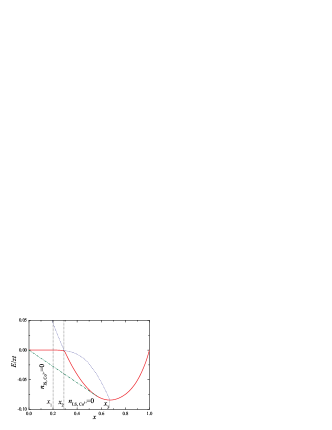
Figure 1: (Color online) The energies of type 1 and 2 states as function of doping $x$. The red solid curve corresponds to the more favorable in energy homogeneous state, whereas the states with higher energies are shown by blue dashed lines (see the text). The green dot-dashed line corresponds to the energy of an inhomogeneous state, obtained by Maxwell construction. $\Delta_{1}/zt=0.2$.

Let us denote the state similar to that in Ref. myPRL, (that is the state with coexisting LS and IS Co³⁺ ions) as a type 1 state, and the state without LS Co³⁺ as type 2 state. The energies of these two states as function of doping $x$ are shown in Fig. 1 at $\Delta_{1}/zt=0.2$ ($z=6$ is the number of nearest neighbors). The type 2 state becomes favorable at $x>x_{2}$. Note that at $x>x_{3}$ both states, 1 and 2, are equivalent. We can see that at $x<x_{1}$ there are no electrons promoted to the $e_{g}$ level ($n^{e}=0$), see Fig. 2.

At $x>x_{1}$ the number of $e_{g}$ electrons gradually grows. In the absence of type 2 state, this growth would continue up to $x=x_{3}$ when all Co³⁺ ions would turn to the intermediate spin state. At $x=x_{2}$, however, the type 2 state becomes favorable in energy, and the jump-like transition to this state occurs. The ground state energy $E$ for the homogeneous system as function of $x$ is shown in Fig. 1 by red solid curve. At the same time, it is clear from this figure that in the doping range $0<x\lesssim x_{3}$ the inhomogeneous state, being a mixture of states with $n^{h}=1$ and $n^{e}=0$, is more favorable. The energy of this mixed state is shown in Fig. 1 by the green dot-dashed line.

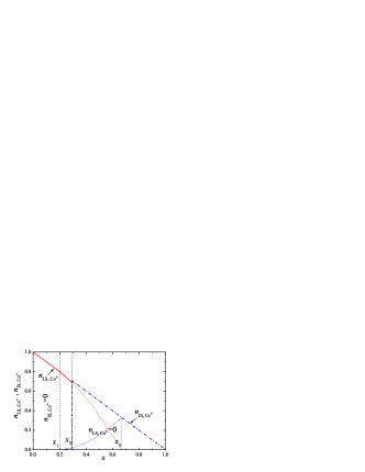
Figure 2: (Color online) The densities of Co³⁺ ions in intermediate- ($n^{e}=n_{\text{IS, Co}^{3+}}$) and low-spin ($1-n^{h}=n_{\text{LS, Co}^{3+}}$) homogeneous states as a function of $x$ at $\Delta_{1}/zt=0.2$. At $x_{1}<x<x_{2}$, both spin states of Co³⁺ coexist, whereas at $x=x_{2}$, there occurs a jump-like transition to the purely IS state of Co³⁺ ions. Dashed lines illustrate the possible behavior of $n_{\text{IS, Co}^{3+}}$ and $n_{\text{LS, Co}^{3+}}$ for the type I state similar to that described in Ref. myPRL, .

The densities of Co³⁺ ions in intermediate-spin ($n^{e}$) and low-spin ($1-n^{h}$) states as a function of $x$ are shown in Fig. 2 by blue dot-dashed and red solid curves, respectively. We see a jump-like increase of $n^{e}$ at $x_{2}$, when the homogeneous type 2 state would become favorable. The behavior of $n^{e}$ and $1-n^{h}$ at $x>x_{2}$ in the absence of type 2 state are shown by thin blue and red dashed lines, respectively.

At a small band filling, $n^{e}\ll 1$, we can write an approximate explicit expression for the total energy $E$ assuming that the Fermi surface is spherical

$$E\simeq\Delta_{1}n^{e}-tzn^{e}n^{h}+\frac{3t}{5}\left(36\pi^{4}n^{h}\right)^{1/3}(n^{e})^{5/3}\,.$$ (10)

The density $n^{e}$ of itinerant electrons is determined by minimization of Eq. (10) with respect to $n^{e}$ taking into account that $n^{h}=x+n^{e}$. It can be easily shown that the solution for the energy minimum corresponding to $n^{e}\neq 0$ can exist only if $\Delta_{1}<tzx$. This means that at $\Delta_{1}/tz>1$ the LS Co³⁺ ions can not be promoted to the IS state at any doping $x$.

The dependence of $n^{e}$ on doping $x$ determines the behavior of magnetic moment of Co ions. Indeed, the LS Co³⁺ ions correspond to zero magnetic moment, $S=0$, while the doping leads to creation of LS Co⁴⁺ ions ($S=1/2$) and also provides the promotion of some Co³⁺ ions to the IS state ($S=1$). So, the data presented in Fig. 2 could be redrawn in terms of magnetic moment per dopant (or, in other words, per Co⁴⁺), see Fig. 3. For the homogeneous state, we see in Fig. 3 that the jump-like transition in the density $n^{e}$ of itinerant electrons manifests itself in a jump of magnetic moment. At the same time, in the phase-separated state, the magnetic moment per Co⁴⁺ ion remains constant since both the content of the phase with IS Co³⁺ and the number of Co⁴⁺ ions are proportional to $x$. The value of magnetic moment per Co⁴⁺ is determined by the value of $x$, where the green dot-dashed line in Fig. 1 touches the curve corresponding to the energy of the homogeneous state. Both the height of the jump for the magnetic moment in the homogeneous state and the value of magnetic moment per Co⁴⁺ in the phase-separated state depend drastically in the parameters of the model, especially on the hopping integral $t$. In Fig. 3, we see that the increase in $t$ by a factor of two leads to a pronounced growth of both mentioned values. Note here that the values of magnetic moment under discussion correspond to macroscopic phase separation, that is the characteristic sizes of inhomogeneities are much larger than the lattice constant. It is indeed so at relatively large $x$ (exceeding the percolation threshold for the phase with itinerant charge carriers). At small $x$, it is naturally to expect that the phase-separated system will consist of small droplets (spin-state polarons) containing only one Co⁴⁺ ion surrounded by IS Co³⁺. In the latter case, the magnetic moment per Co⁴⁺ should be larger than that corresponding to the macroscopic phase separation. This could be the case for spin polarons in low-doped La_1-xSr_xCoO₃ observed in Ref. Podles08, , where the polarons with the magnetic moment equal to $13\mu_{B}$ seem to be the most probable. From our considerations, one should expect that the value of the moment per of Co⁴⁺ should become smaller with the increase of doping $x$. The exact calculations for small clusters also demonstrate that in a suitable range of parameters the saturated magnetic moment can exist at relatively low temperatures also in atomic-size doped clusters of various geometries Kochar2 .

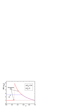
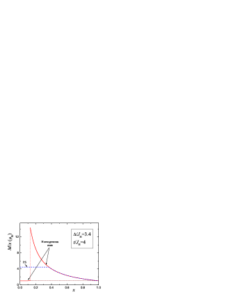
Figure 3: (Color online) Magnetic moment per one Co⁴⁺ ion versus doping $x$ at different values of the hopping integral $t$. The red curves correspond to the homogeneous states. The behavior $M$ in the phase-separated state is shown by the blue dashed line.

Thus, we demonstrated that the spin-state transitions in hole-doped cobaltites can be described based on the model involving the coexistence and competition of localized and itinerant electron states. In contrast to the similar model for manganites myPRL ; myPRB , this model allows the possibility of a jump-like transition to the purely itinerant state corresponding in the case of cobaltites to the LS $\rightarrow$IS transition for all Co³⁺ ions. However, at lower doping, before reaching this homogeneous metallic state with all Co ions magnetic, the phase-separated state comes into play, in which only a part of Co³⁺ ions is promoted to the IS state, doped holes being located in these regions. Experimental data on La_1-xSr_xCoO₃ Rivas ; Loshk ; Louca ; Leighton06 ; Leighton07 ; Podles08 seem to be in agreement with this picture.

IV Charge transfer effects and spin-state transitions: The case of HS-HS ground state for isolated ions

Let us now discuss the situation at $\Delta<2J_{H}$, when in the absence of electron hopping it is favorable for both Co³⁺ and Co⁴⁺ to be in the HS state. The charge transfer becomes possible only if we promote a hole to the $e_{g}$ level of Co⁴⁺ and transform such an ion from HS to IS state.

So, in this case, instead of electron hopping from IS Co³⁺ to LS Co⁴⁺, we have the electron hopping from the HS Co³⁺ to IS Co⁴⁺, or the hole hopping from IS Co⁴⁺ to HS Co³⁺ (this representation is more convenient here). Using this analogy, we can choose the HS state of Co⁴⁺ as a new vacuum state and write relationships similar to (III) and (2) as

$$|0\rangle = |\textrm{Co}_{HS}^{4+}\rangle,\quad\tilde{E}^{(vac)}=E_{1}+2\Delta-6J_{H}=\tilde{E}_{0},$$

$$\tilde{c}_{\bf{n}}^{{\dagger}}|0\rangle = |\textrm{Co}^{5+}\rangle,\quad E^{(5+)}=\tilde{U}^{\prime},$$

$$\tilde{a}_{\bf{n}}^{{\dagger}}|0\rangle = |\textrm{Co}_{HS}^{3+}\rangle,\quad E^{(e)}=E_{0}+2\Delta-4J_{H}=\tilde{E}_{1},$$

$$\tilde{a}_{\bf{n}}^{{\dagger}}\tilde{c}_{\bf{n}}^{{\dagger}}|0\rangle = |\textrm{Co}_{IS}^{4+}\rangle,\,E_{IS}^{(4+)}=E_{0}+\Delta-2J_{H}=\tilde{E}_{2}.$$ (11)

The corresponding single-site Hamiltonian can be found by the following substitution in (3) and (4): $E_{0},E_{1},E_{2},U\rightarrow\tilde{E}_{0},\tilde{E}_{1},\tilde{E}_{2},\tilde{U}$ and also $n^{e}_{{\bf n}}\rightarrow\tilde{n}^{h}_{{\bf n}},n^{h}_{{\bf n}}\rightarrow\tilde{n}^{e}_{{\bf n}}$.

As a result, we can rewrite the Hamiltonian (5) in the following form

$$H = \sum_{\bf{n}}[\tilde{E}_{0}+(\tilde{E}_{0}-\tilde{E}_{1}-\mu)(\tilde{n}_{\bf{n}}^{e}-\tilde{n}_{\bf{n}}^{h})]+$$ (12)

$$+\Delta_{2}\sum_{{\bf n}}\tilde{n}^{h}_{{\bf n}}+\tilde{U}\sum_{{\bf n}}\tilde{n}^{h}_{{\bf n}}(1-\tilde{n}^{n}_{{\bf n}})$$

$$-t\sum_{\langle{\bf n}{\bf m}\rangle}\left(\tilde{c}^{{\dagger}}_{{\bf n}}\tilde{c}_{{\bf m}}+h.c.\right)\,.$$

Here, $\Delta_{2}=4J_{H}-\Delta$ is the energy difference between the IS and HS Co⁴⁺ ions, $\tilde{c}^{{\dagger}}_{{\bf n}}$, $\tilde{c}_{{\bf n}}$ are creation and annihilation operators for a hole promoted to the $e_{g}$ level of IS Co⁴⁺ at site $\bf n$, $\tilde{n}^{h}_{{\bf n}}=\tilde{c}^{{\dagger}}_{{\bf n}}\tilde{c}_{{\bf n}}$, and $\tilde{n}^{e}_{{\bf n}}=\tilde{a}^{{\dagger}}_{{\bf n}}\tilde{a}_{{\bf n}}$ is the operator describing the number ($0$ or $1$) of additional localized $t_{2g}$ electrons at site ${\bf n}$ ($\tilde{a}^{{\dagger}}_{{\bf n}}$, $\tilde{a}_{{\bf n}}$ are creation and annihilation operators for such electrons). The average numbers of electrons and holes per site obey now the relationship $\tilde{n}^{e}-\tilde{n}^{h}=1-x$.

In this case, the energy per site (6) can be rewritten as

$$E^{(2)}=E_{0}(1-x)+E_{1}x+\langle H_{2}\rangle/N\,,$$ (13)

where

$$H_{2} = \sum_{{\bf n}}\left(2\Delta-6J_{H}+2J_{H}(\tilde{n}_{\bf{n}}^{e}-\tilde{n}_{\bf{n}}^{h})\right)+$$ (14)

$$\Delta_{2}\sum_{{\bf n}}\tilde{n}_{\bf{n}}^{h}+\tilde{U}\sum_{{\bf n}}\tilde{n}^{h}_{{\bf n}}(1-\tilde{n}^{n}_{{\bf n}})$$

$$-t\sum_{\langle{\bf n}{\bf m}\rangle}\left(\tilde{a}^{{\dagger}}_{{\bf n}}\tilde{a}_{{\bf m}}+h.c.\right)\,.$$

Note that the difference $E^{(2)}-E^{(1)}$, does not depend on the choice of $E_{0}$ and $E_{1}$, this fact will be helpful in constructing the phase diagrams in the next section.

Thus, the behavior of the system energy and charge carrier densities, $\tilde{n}^{e}$ and $\tilde{n}^{h}$ are similar to those shown in Figs. 1 and 2. In these figures we should replace $n^{h}\to\tilde{n}^{e}$, $n^{e}\to\tilde{n}^{h}$, and $x\to 1-x$, that is, the densities of Co³⁺ ions in IS ($n^{e}=n_{\text{IS,Co}^{3+}}$) and LS ($1-n^{h}=n_{\text{LS, Co}^{3+}}$) states become here the densities of Co⁴⁺ ions in IS ($\tilde{n}^{h}=n_{\text{IS, Co}^{4+}}$) and HS ($1-\tilde{n}^{e}=n_{\text{HS, Co}^{4+}}$) states. Note also that such an exact similarity between the LS-LS and HS-HS cases appears since we, in fact, deal with the spinless fermions (the spins of charge carriers are parallel). So, we have an electron-hole symmetry between an empty $e_{g}$ level at LS Co³⁺ and a completely occupied such level at HS Co³⁺.

V Phase diagrams

Based on the results of the previous sections, we can summarize the behavior of the system as function of doping at different values of the $\Delta/J_{H}$ ratio and to draw the corresponding phase diagram. The form of this phase diagram depends drastically on the characteristic values of the hopping integral $t$. The general features of the evolution of the system with doping from one homogeneous state to another are illustrated in Fig. 4. At rather small $t$ ($t/J_{H}\lesssim 1$), see Fig. 4a, we have clearly defined regions of the phase diagram corresponding to $\Delta>3J_{H}$ and $\Delta<2J_{H}$ (corresponding to the situations discussed in sections III and IV, respectively). In each of these regions, the variation of doping leads to the transitions between the phase with only localized carriers to the phase when some charge carriers are delocalized and, eventually, to the phase when all charge carriers are itinerant. These two regions, with $\Delta>3J_{H}$ and $\Delta<2J_{H}$, are separated by the phase with Co³⁺ in LS ($S=0$) and Co⁴⁺ in HS ($S=5/2$) states,with the charge carriers localized because of the spin blockade SpinBlock . At larger $t$ ($t/J_{H}\gtrsim 1$), see Fig. 4b, the latter intermediate region collapses at a certain doping range, and a direct spin-state transition between the phases with fully delocalized charge carriers becomes possible.

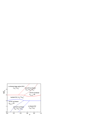
(a) $\quad t/J_{H}=1$

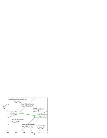
(b) $\quad t/J_{H}=1.5$

Figure 4: (Color online) Possible homogeneous states of the system under study at different values of the hopping integral $t$. The boundaries between analogous phases in the upper and lower parts of the phase diagram are shown by the same lines (solid, dashed, or dot-and-dash).

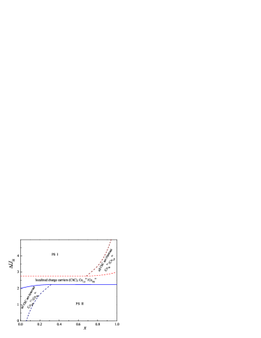
(a) $\quad t/J_{H}=1$

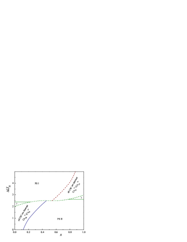
(b) $\quad t/J_{H}=1.3$

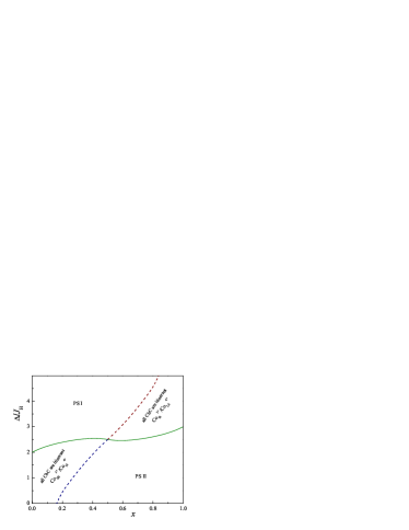
(c) $\quad t/J_{H}=1.5$

Figure 5: (Color online) Phase diagrams including the phase-separated states of the system under study at different values of hopping integral $t$. PS I is the phase-separated state including the regions without itinerant charge carriers, corresponding to LS Co³⁺, and those with completely delocalized charge carries promoted to IS Co³⁺. PS II is the similar phase-separated state where the regions with and without itinerant charge carriers correspond to IS Co⁴⁺ and HS Co⁴⁺, respectively. Regions 1 at panel (b) correspond to the charge carriers located at HS Co⁴⁺ and LS Co³⁺ where the charge transfer between Co sites is suppressed due to the spin blockade.

The form of the phase diagram changes if we take into account the possibility of phase separation. The corresponding phase diagrams drawn at different values of $t/J_{H}$ are shown in Fig. 5. We see that instead of phases with partially and fully delocalized charge carriers, there appears a broad regions of phase separation where the domains of fully localized and fully delocalized charge carriers are intermixed. Again, at rather small $t$ ($t/J_{H}\lesssim 1$), we have and intermediate region where the charge carries are localized at any doping level (with Co³⁺ and Co⁴⁺ in LS and HS states, respectively). This intermediate region gradually disappears with the growth of the hopping integral $t$.

Let us note here that the phase diagram along the $\Delta$ axis could be reproduced varying the average ionic radius of the rare-earth ions in cobaltites (see, e.g. Refs. Fujita, , Wang, ).

Note also that the long-range Coulomb interaction related to the charge disproportionalization in the phase-separated state can reduce the doping range of the phase separation and modify the form of the phase diagram shown in Fig. 5.

VI Conclusions

Based on a simplified model of a strongly correlated electron system with spin-state transitions, we demonstrated a tendency to the phase separation for doped perovskite cobaltites in a wide range of doping levels. The phase diagram including large regions of inhomogeneous phase-separated states was constructed in the plane of parameters doping $x$ versus $e_{g}-t_{2g}$ energy splitting $\Delta$. The form of the phase diagram turns out to be strongly dependent on the ratio of of the electron hopping integral $t$ and and the Hund’s rule coupling constant $J_{H}$.

Here, we did not analyzed in detail the possible structure of the phase-separated state. However, for the corresponding model describing doped manganites, the calculations myPRL and numerical simulations Ramakr taking into account the surface and long-range Coulomb contributions to the total energy lead to the characteristic size of nanoscale inhomogeneities of the order of several lattice constants.

References

- (1) Also at the Department of Physics, Loughborough University, Leicestershire, LE11 3TU, UK.
- (2) K.I. Kugel, A.L. Rakhmanov, and A.O. Sboychakov, Phys. Rev. Lett. 95, 267210 (2005).
- (3) E. Dagotto, Nanoscale Phase Separation and Colossal Magnetoresistance: The Physics of Manganites and Related Compounds (Springer-Verlag, Berlin, 2003).
- (4) E. Nagaev, Colossal Magnetoresistance and Phase Separation in Magnetic Semiconductors (Imperial College Press, London, 2002).
- (5) M.Yu. Kagan and K.I. Kugel, Usp. Fiz. Nauk. 171, 577 (2001) [Physics - Uspekhi 44, 553 (2001)].
- (6) K.I. Kugel, A.L. Rakhmanov, A.O. Sboychakov, and D.I. Khomskii, Phys. Rev. B78, 155113 (2008).
- (7) K.I. Kugel, A.O. Sboychakov, and D.I. Khomskii, J. Supercond. Nov. Magn. 22, 147 (2009).
- (8) P.M. Raccah and G.B. Goodenough, Phys. Rev. 155, 932 (1967).
- (9) S. Yamaguchi, Y. Okimoto, H. Taniguchi, and Y. Tokura, Phys. Rev. B53, R2926 (1996).
- (10) S. Yamaguchi, Y. Okimoto, and Y. Tokura, Phys. Rev. B55, R8666 (1997).
- (11) M.A. Korotin, S.Yu. Ezhov, I.V. Solovyev, V.I. Anisimov, D.I. Khomskii, and G.A. Sawatzky, Phys. Rev. B54, 5309 (1996).
- (12) M. Pouchard, A. Villesuzanne, and J.P. Doumerc, J. Solid State Chem. 162, 282 (2001).
- (13) D.I. Khomskii and U. Löw, Phys. Rev. B69, 184401 (2004).
- (14) P.W. Anderson and H. Hasegawa, Phys. Rev. 100 675 (1955).
- (15) P.G. de Gennes, Phys. Rev. 118 141 (1960).
- (16) L.N. Bulaevskii and D.I. Khomskii, Zh. Eksp. Teor. Fiz. 52, 1603 (1967) [Sov. Phys. JETP 25, 1067 (1967)].
- (17) L.N. Bulaevskii, E.L. Nagaev, and D.I. Khomskii, Zh. Eksp. Teor. Fiz. 54, 1562 (1968) [Sov. Phys. JETP 27, 836 (1968)].
- (18) E.L. Nagaev, Pis ma Zh. Eksp. Teor. Fiz. 6, 484 (1967) [JETP Lett. 6, 18 (1967)].
- (19) T. Kasuya, A. Yanase, and T. Takeda, Solid State Commun. 8, 1543 (1970).
- (20) R. Kilian and G. Khaliullin, Phys. Rev. B60, 13458 (1999).
- (21) T. Mizokawa, D.I. Khomskii, and G.A. Sawatzky, Phys. Rev. B61, R3776 (2000); Phys. Rev. B63, 024403 (2001).
- (22) A. Maignan, V. Caignaert, B. Raveau, D. Khomskii, and G. Sawatzky, Phys. Rev. Lett. 93, 026401 (2004).
- (23) R. Caciuffo, D. Rinaldi, G. Barucca, J. Mira, J. Rivas, M.A. Señarís-Rodríguez, P.G. Radaelli, D. Fiorani, and J.B. Goodenough, Phys. Rev. B59, 1068 (1999).
- (24) N.N. Loshkareva, E.A. Gan shina, B.I. Belevtsev, Yu.P. Sukhorukov, E.V. Mostovshchikova, A.N. Vinogradov, V.B. Krasovitsky, and I.N. Chukanova, Phys. Rev. B68, 024413 (2003).
- (25) D. Phelan, Despina Louca, K. Kamazawa, S.-H. Lee, S. Rosenkranz, Y. Motome, M.F. Hundley, J.F. Mitchell, S.N. Ancona, and Y. Moritomo, Phys. Rev. Lett. 97, 235501 (2006).
- (26) S.R. Giblin, I. Terry, D. Prabhakaran, A.T. Boothroyd, J. Wu, and C. Leighton, Phys. Rev. B74, 104411 (2006).
- (27) C. He, M.A. Torija, J. Wu, J.W. Lynn, H. Zheng, J.F. Mitchell, and C. Leighton, Phys. Rev. B76, 014401 (2007).
- (28) A. Podlesnyak, M. Russina, A. Furrer, A. Alfonsov, E. Vavilova, V. Kataev, B. Büchner, Th. Strässle, E. Pomjakushina, K. Conder, and D.I. Khomskii, Phys. Rev. Lett. 101, 247603 (2008).
- (29) M.Yu. Kagan, D.I. Khomskii, and M.V. Mostovoy, Eur. Phys. J. B 12, 217 (1999).
- (30) M.Yu. Kagan, K.I. Kugel, and D.I. Khomskii, Zh. Eksp. Teor. Fiz. 120, 470 (2001) [JETP 93, 415 (2001)].
- (31) A.O. Sboychakov, K.I. Kugel,and A.L. Rakhmanov, Phys. Rev. B74, 014401 (2006).
- (32) J. Baier, S. Jodlauk, M. Kriener, A. Reichl, C. Zobel, H. Kierspel, A. Freimuth, and T. Lorenz, Phys. Rev. B71, 014443 (2005).
- (33) L.M. Falicov and J.C. Kimball, Phys. Rev. Lett. 22, 997 (1969).
- (34) V.B. Shenoy, T. Gupta, H.R. Krishnamurthy, and T.V. Ramakrishnan, Phys. Rev. Lett. 98, 097201 (2007).
- (35) A.N. Kocharian, G.W. Fernando, K. Palandage, and J.W. Davenport, Phys. Lett. A 373, 1074 (2009).
- (36) J. Hubbard, Proc. Roy. Soc. (London) A276, 238 (1963).
- (37) A.N. Kocharian, G.W. Fernando, K. Palandage, and J.W. Davenport, Phys. Rev. B78, 075431 (2008).
- (38) T. Fujita, S. Kawabata, M. Sato, N. Kurita, M. Hedo, and Y. Uwatoko, J. Phys. Soc. Japan 74, 2294 (2005).
- (39) G.Y. Wang, X.H. Chen, T. Wu, G. Wu, X.G. Luo, and C.H. Wang, Phys. Rev. B74, 165113 (2006).