Evaluation of Mutual Information Estimators for Time Series

Abstract

We study some of the most commonly used mutual information estimators, based on histograms of fixed or adaptive bin size, $k$-nearest neighbors and kernels, and focus on optimal selection of their free parameters. We examine the consistency of the estimators (convergence to a stable value with the increase of time series length) and the degree of deviation among the estimators. The optimization of parameters is assessed by quantifying the deviation of the estimated mutual information from its true or asymptotic value as a function of the free parameter. Moreover, some common-used criteria for parameter selection are evaluated for each estimator. The comparative study is based on Monte Carlo simulations on time series from several linear and nonlinear systems of different lengths and noise levels. The results show that the $k$-nearest neighbor is the most stable and less affected by the method-specific parameter. A data adaptive criterion for optimal binning is suggested for linear systems but it is found to be rather conservative for nonlinear systems. It turns out that the binning and kernel estimators give the least deviation in identifying the lag of the first minimum of mutual information from nonlinear systems, and are stable in the presence of noise.

Keywords: mutual information, probability density, time series, nonlinear systems

running title: Mutual Information Estimators

1 Introduction

Mutual information (MI) is a nonlinear measure used in many aspects of time series analysis, best known as a criterion to select the appropriate delay for state space reconstruction [Kantz & Schreiber, 1997]. It is also used to discriminate different regimes of nonlinear systems [Hively et al., 2000; Naa et al., 2002; Wicks et al., 2007] and to detect phase synchronization [Schmid et al., 2004; Kreuz et al., 2007]. Besides nonlinear dynamics, it is used in various statistical settings, mainly as a distance or correlation measure in data mining, e.g. in independent component analysis and feature-based clustering [Tourassi et al., 2001; Priness et al., 2007].

Any estimate of MI, either between two variables or as a function of delay for time series, is (almost always) positively biased [Treves & Panzeri, 1995; Moddemeijer, 1989; Paninski, 2003; Micheas & Zografos, 2006]. For numerical-valued variables, MI increases with finer partition depending on the underlying distribution and the sample size. Beyond the classical domain partitioning, other schemes have been used to estimate the densities inherent in the measure of mutual information, e.g. kernels, B-splines and $k$-nearest neighbors [Moon et al., 1995; Diks & Manzan, 2002; Daub et al., 2004; Kraskov et al., 2004].

There are generally few analytic results on MI. Expressions of MI in terms of the correlation coefficient are obtained for some known distributions, e.g. Gaussian and Gamma distribution [Pardo, 1995; Hutter & Zaffalon, 2005]. Some statistical results on the mean, variance and bias of the MI estimator using fixed partitioning can be found in [Roulston, 1997; Abarbanel et al., 2001], but the distribution of any MI estimator is not known in general. For chaotic systems in particular, the discontinuity of the density function of their variables does not allow for an analytic derivation of the statistics of MI estimators. Therefore, comparisons of MI estimators relies on simulation studies. In some studies the estimators are tested in identifying correctly the lag of the first minimum of MI [Moon et al., 1995; Cellucci et al., 2005]. Another performance criterion is the bias of estimators in the case of Gaussian processes, where the true MI is known [Cellucci et al., 2005; Trappenberg et al., 2006].

MI estimation involves one and two dimensional density estimation. Density estimation has been studied extensively and different methods have been suggested and compared in the statistical literature, e.g. see [Scott, 1979; Freedman & Diaconis, 1981; Silverman, 1986], but it is still to be investigated whether these methods and the suggested criteria for the selection of method specific parameters are also suitable for MI estimation. This is the main objective of this study. MI estimators have also been compared to other linear or nonlinear correlation measures [Palus, 1995; Steuer et al., 2002; Daub et al., 2004], but we do not pursue this here as direct comparison is not possible due to the different scaling of the measures, even after normalization. There are some comparative studies on the MI estimators and the selection of their parameters, as well as on their performance on both linear and nonlinear dynamical systems [Wand & Jones, 1993; Steuer et al., 2002; Nicolaou & Nasuto, 2005; Khan et al., 2007]. Here, we extend these studies, we evaluate some of the most commonly used MI estimators, examine their consistency and optimize the selection of their parameters including criteria for parameter selection suggested in the literature. As the estimation depends on the underlying time series we use Monte-Carlo simulations on systems of white noise of different distributions, stochastic linear systems and dynamical non-linear systems (maps and flows of varying complexity). The performance of each estimator is examined with respect to the time series length, the distribution of noise and the noise level in the systems.

We study here the performance of three types of estimators, i.e. estimators based on histograms (with fixed or adaptive bin size), $k$-nearest neighbors and kernels. All estimators vary in the estimation of the densities at local regions and we investigate the optimal parameter for the determination of the two-dimensional partitioning. Based on the simulation results, we propose optimal parameters for each MI estimator with regard to the complexity of the system, the observational noise level and the time series length.

The structure of the paper is as follows. In Sec. 2, we briefly discuss the estimators considered in this study and in Sec. 3 we present the evaluation procedure and the simulated systems. In Sec. 4, we give quantitative results on the dependence of the estimators on the parameters, time series length and noise, we propose optimal parameter selection and compare the different MI estimators. Finally, in Sec. 5 we discuss the results and draw conclusions.

2 Mutual Information Estimators

MI is a measure of mutual dependence between two random variables and quantifies the amount of uncertainty about one variable reduced when knowing the other. The MI of two continuous random variables $X,Y$ has the form

$${\cal I}(X,Y)=\int_{X}\int_{Y}f_{X,Y}(x,y)\log_{a}{\frac{f_{X,Y}(x,y)}{f_{X}(x)f_{Y}(y)}}\mbox{d}x\mbox{d}y,$$ (1)

where $f_{X,Y}(x,y)$ is the joint probability density function (pdf) of $X$ and $Y$, whereas $f_{X}(x)$ and $f_{Y}(y)$ are the marginal pdfs of $X$ and $Y$, respectively. The units of information of ${\cal I}(X,Y)$ depend on the base $a$ of the logarithm, e.g. bits for the base $2$ logarithm and nats for the natural logarithm.

Assuming a partition of the domain of $X$ and $Y$, the double integral in Eq.(1) becomes a sum over the cells of the two-dimensional partition

$${\cal I}(X,Y)=\sum_{i,j}p_{X,Y}(i,j)\log_{a}{\frac{p_{X,Y}(i,j)}{p_{X}(i)p_{Y}(j)}},$$ (2)

where $p_{X}(i)$, $p_{Y}(j)$, and $p_{X,Y}(i,j)$ are the marginal and joint probability mass functions over the elements of the one and two-dimensional partition. In the limit of fine partitioning the expression in Eq.(2) converges to Eq.(1). This may partly justify the abuse of notation of MI for the continuous and the discretized variables. It is always ${\cal I}(X,Y)\geq 0$, with equality holding for independent variables, and ${\cal I}(X,Y)\leq H(X)\leq\log_{a}{n}$ (Jensen inequality), where $H(X)=\sum_{i=1}^{n}p(x_{i})\log_{a}p(x_{i})$ is the Shannon entropy of $X$. For a time series $\{X_{t}\}_{t=1}^{n}$, sampled at fixed times $\tau_{s}$, MI is defined as a function of the delay $\tau$ assuming the two variables $X=X_{t}$ and $Y=X_{t-\tau}$, i.e. ${\cal I}(\tau)={\cal I}(X_{t},X_{t-\tau})$.

The Shannon entropy is always misestimated due to finite sample effects [Grassberger, 1988; Kantz & Shürmann, 1996], but we do not discuss MI in terms of entropies here as the estimation of MI boils down to the estimation of the densities in Eq.(1) or probabilities in Eq.(2). The estimators of MI, denoted $I(\tau)$, differ in the estimation of the marginal and joint probabilities or densities, using binning [Fraser & Swinney, 1986; Darbellay & Vajda, 1999], kernels [Silverman, 1986; Moon et al., 1995] or correlation integrals [Diks & Manzan, 2002], $k$-nearest neighbors [Paninski, 2003; Kraskov et al., 2004], $B$-splines [Daub et al., 2004] or the Gram-Charlier polynomial expansion [Blinnikov & Moessner, 1998]. All these estimators depend on at least one parameter. We present bellow the three first estimators that are most widely used.

2.1 Binning estimators

The most common MI estimator is the naive equidistant binning estimator (ED) that regards the partition of the domain of each variable into a finite number $b$ of discrete bins (equidistant partitioning). The probability at each cell or bin is estimated by the corresponding relative frequency of occurrence of the samples in the cell or bin. The number of bins for each variable is the same, so that the parameter to be optimized is the number of bins for the partition or equivalently the bin width. The computation of this MI estimator is straightforward as it is directly estimated from the one and two dimensional histograms.

A second binning estimator is the equiprobable binning estimator (EP), which is derived by partitioning the domain of each variable in $b$ bins of the same occupancy (equiprobable partitioning) but different width. The equiprobable partitioning actually transforms the sample univariate distribution to discrete uniform with $b$ components minimizing the effect of the univariate distribution on the estimation.

Fraser & Swinney [1986] suggested an estimator using an adaptive partitioning. This method constructs a locally adaptive partition of the two-dimensional plane. It starts with a partition of equiprobable bins for each variable and makes finer partition in areas where the joint probability density is non-uniform until the joint distribution on the cells is approximately uniform. The final partition is finer in dense regions whereas less occupied regions are covered with larger cells. It was found in [Palus, 1993; Cellucci et al., 2005] that this complex algorithm does not substantially improve the binning estimator and requires large data sets to gain accuracy; therefore it is not included in the current evaluation.

A different estimator making use of adaptive partitioning (AD) is proposed by Darbellay & Vajda [1999]. The partition consists of rectangles specified by marginal empirical quantiles, which are not uniform in the sense that they are not made of a grid of vertical and horizontal lines, irrespectively of whether these lines are equally spaced or not. The AD estimator builds such a partition in a way that it achieves conditional independence on the rectangles of the partition. The advantage of this estimator is that it is data-adaptive and does not a priori determine the number of bins in the partition. The AD estimator has a direct dependence on $n$, which determines the roughness of the partitioning in a somehow automatic way. In the abundance of data, the AD estimator reaches a very fine partition that satisfies the independence condition in each cell, so that the total number of cells is very large and analogous to a fixed-partition with a respectively large $b$. Note that the dependence of AD on $n$ is not comparable to that of the fixed-bin estimators because it involves a change of partitioning with $n$.

For any binning scheme, the MI estimator $I(\tau)$ is given by Eq.(2) where the variables are $(X,Y)=(X_{t},X_{t-\tau})$, the sum is referred to the partition of the two-dimensional domain of $(X_{t},X_{t-\tau})$ and $p_{X_{t}}$, $p_{X_{t-\tau}}$, $p_{{X_{t}},X_{t-\tau}}$ are the marginal and joint probability distributions defined for each cell of the partition.

2.2 $k$-nearest neighbor estimator

Kraskov et al. [2004] proposed an MI estimator (KNN) that uses the distances of $k$-nearest neighbors to estimate the joint and marginal densities. For each reference point from the bivariate sample, a distance length is determined so that the $k$ nearest neighbors are within this distance length. Then the number of points within this distance from the reference point gives the estimate of the joint density at this point and the respective neighbors in one-dimension give the estimate of the marginal density for each variable. The algorithm uses discs (or squares depending on the metric) of a size adapted locally and then uses the corresponding size in the marginal subspaces, so in some sense the estimator is data adaptive. Still, it involves as a free parameter the number of neighbors $k$. Note that a large $k$ regards a small $b$ of the fixed binning estimators. However, the estimator does not use a fixed neighborhood size and therefore there is not a clear association of $k$ and $b$. The KNN estimator is data efficient, adaptive, has minimal bias and is recommended for high-dimensional data sets [Kraskov et al., 2004]. It requires an additional computational cost for the search of the $k$ neighbors.

2.3 Kernel density estimator

The kernel density MI estimator (KE) uses a smooth estimate of the unknown probability density by centering kernel functions at the data samples; kernels are used to obtain the weighted distances [Silverman, 1986; Moon et al., 1995]. The kernels essentially weigh the distance of each point in the sample to the reference point depending on the form of the kernel function and according to a given bandwidth $h$, so that a small $h$ produces details in the density estimate but may loose in accuracy depending on the data size.

KE estimator has two free parameters, the bandwidth $h_{1}$ for the marginal densities of $X$ and $Y$, and the bandwidth $h_{2}$ for the joint density of $(X,Y)$. The bandwidth $h_{1}$ is related to $b$ of the fixed binning estimators by an inverse relation, e.g. a rectangular kernel assigns a bin centered at the reference point. Its advantage over binning estimators is that the location of the bins is not fixed. Among the different kernel functions, Gaussian kernels are most commonly used and we use them here as well. A kernel density estimator with Gaussian kernel function and a fixed bandwidth $h$ at a point $\textbf{x}\in R^{d}$ is

$$f(\textbf{x})=\frac{1}{{{(2\pi)}^{d/2}h^{d}\mbox{det}(\textbf{S})^{1/2}}}\sum_{i=1}^{n^{\prime}}\exp\left({-\frac{{(\textbf{x}-\textbf{x}_{i})}^{\tau}\textbf{S}^{-1}(\textbf{x}-\textbf{x}_{i})}{2h^{2}}}\right),$$ (3)

where S is the data covariance matrix and $n^{\prime}$ is the number of the $d$-dimensional vectors [Moon et al., 1995].

3 Simulation Setup

The evaluation of the estimators is assessed by Monte-Carlo simulations on white noise, linear systems and chaotic systems of different complexity, listed in Table 1.
===============================================
TABLE 1 *** To be placed here ***
===============================================
A Gaussian and a skewed Gamma distribution are used to generate white noise time series, whereas for linear systems, the autoregressive model AR(1) and autoregressive moving average ARMA(1,1) are used with coefficients as given in Table 1, assuming both Gaussian and Gamma input white noise. The non-linear chaotic systems are the Henon map [Henon, 1976]

$$x_{t}=1-ax_{t-1}^{2}+bx_{t-2},$$

the Ikeda map [Ikeda et al., 1980]

$$x_{t} = a+b(x_{t-1}\cos u_{t-1}-y_{t-1}\sin u_{t-1})$$

$$y_{t} = b(x_{t-1}\sin u_{t-1}+y_{t-1}\cos u_{t-1}),$$

where $u_{t}=\kappa-\frac{\eta}{1+x_{t}^{2}+y_{t}^{2}}$, and the Mackey-Glass differential system [Mackey & Glass, 1977]

$$\frac{\mbox{d}x}{\mbox{d}t}=\frac{0.2x_{t-\Delta}}{1+x_{t-\Delta}^{10}}-0.1x_{t}$$

where the delay $\Delta$ accounts for the system complexity. We use here $\Delta=17$ and $\Delta=30$ for low-dimensional chaos of fractal dimension about 2 and 3, respectively, and $\Delta=100$ for high-dimensional chaos of fractal dimension about 7. Observational white noise at different levels is also assumed for the chaotic systems, given as a percentage of the standard deviation of the noise-free data.

Different lengths $n$ for the generated time series from each system are considered as follows. For white noise and linear systems, $n$ is given in powers of $2$ from $5$ to $13$ and for nonlinear systems from $8$ to $13$. $I(\tau)$ is computed using all methods on $1000$ realizations for each system, noise type or level, and time series length. As all linear systems are of order $1$, MI is computed only for lag $1$. For the nonlinear systems, $I(\tau)$ is computed up to the lag $\tau$ for which $I(\tau)$ levels-off. For the Mackey-Glass system we compute the lag of the first minimum of $I(\tau)$ and specifically for $\Delta=100$ the lag that MI levels-off because it does not exhibit a distinct minimum. For each estimator, $I(\tau)$ is computed for a wide range of values of the free parameter and for specific values determined by standard criteria, which are specified below.

For the binning estimators ED and EP we set the number of bins to $b=2,4,8,16,32,64$. We also consider $10$ commonly used criteria for $b$, given in Table 2.
===============================================
TABLE 2 *** To be placed here ***
===============================================
For the choice of $k$ of $k$-nearest neighbor estimator KNN, Kraskov et al. [2004] propose to use $k=2$ to $4$ (these are also used in [Kreuz et al., 2007; Khan et al., 2007]). However for real world data one should investigate also larger values of $k$. Therefore we use in the simulations a wide range of $k$ values as for $b$, $k=2,4,8,16,32,64$.

Among different kernel functions used in the literature for density estimation, and for MI estimation in particular, the common practice is to use the Gaussian kernel in conjunction with the ”Gaussian” bandwidth of Silverman [1986]

$$\ h={\left(\frac{4}{(d+2)n^{\prime}}\right)}^{1/(d+4)}$$ (4)

($n^{\prime}$ is the number of the $d$-dimensional vectors) or multiples of it [Harrold et al., 2001; Steuer et al., 2002; Khan et al., 2007]. In the estimation of mutual information with kernels, the range of bandwidths is usually not searched and a bandwidth is selected according to a criterion such as the ”Gaussian” bandwidth [Moon et al., 1995; Steuer et al., 2002]. A multiple bandwidth selection scheme for the test for independence is proposed in [Diks & Panchenko, 2008]. Analytic and simulation studies have shown that the choice of the bandwidth is crucial and depends on the data size [Bonnlander & Weigend, 1994; Jones et al., 1996]. Therefore we consider a wide range for the bandwidth $h_{1}$ for one dimension and $h_{2}$ for two dimensions, as for $b$ and $k$. Specifically, for $h_{1}$ we take $15$ values in $[0.01,2]$ at a fixed base-2 logarithmic step and set $h_{2}=h_{1}$ and $h_{2}=\sqrt{2}h_{1}$. The second form for $h_{2}$ accounts for the scaling of the Euclidean metric in $\Re^{2}$, which we use in the simulations. We also consider some well-known criteria for the choice of bandwidths, given in Table 3.
===============================================
TABLE 3 *** To be placed here ***
===============================================
The three first criteria define bandwidth for both one and two-dimensional space. For the other criteria we set $h_{2}$ equal either to $h_{1}$ or $\sqrt{2}h_{1}$.

The true (theoretical) MI ${\cal I}(\tau)$ is not known in general. However, for Gaussian processes ${\cal I}(\tau)$ is given in terms of the autocorrelation function $\rho(\tau)$ as

$${\cal I}(\tau)=-0.5\log(1-{\rho^{2}(\tau)}).$$ (5)

In the lack of the true MI for the other systems, we assume consistency of the estimators and use the asymptotic value of $I(\tau)$ computed on a realization of size $n=10^{7}$. In this computation, we set for the ED and EP estimators $b=64$ (we also computed MI for $b$ up to 256, however MI did not substantially differed), for KNN estimator $k=2$, and for the KE estimator $h_{1}=0.01$ and $h_{2}=h_{1}$. Similar approach for approximating the true MI is used in [Harrold et al., 2001; Cellucci et al., 2005]. We denote $I_{\infty}$ the true or asymptotic MI and use it as reference to compute the accuracy of the different estimators.

We evaluate the estimators and their parameters separately for white noise and linear systems, for the nonlinear maps Henon and Ikeda, and for the Mackey-Glass system. First, we investigate the dependence of the estimators on their free parameter for white noise and linear systems and for different time series lengths giving a total of $L=126$ cases (14 systems and 9 time series lengths). For each estimator, we compute the mean estimated MI $\bar{I}_{c}(l)$ from the $1000$ realizations for each tested value of the free parameter denoted by $c$, where l denotes the system case and $l=1,...,L$. Further, for each $l$ we compute the deviation $dI_{c}(l)=|\bar{I}_{c}(l)-I_{\infty}(l)|$, where $I_{\infty}(l)$ is either the true MI (for Gaussian processes) or the asymptotic value computed from each estimator. All estimators converged to the same MI under proper parameters as obtained for $n$ increasing up to $10^{7}$. Given the asymptotic MI $I_{\infty}(l)$, the optimal parameter values for each case $l$ (system and time series length) is obtained from the minimum deviation $dI_{c}(l)$ with respect to $c$. The estimators are then compared for their optimal parameters by computing the divergence of the mean $I(\tau)$ of each estimator from $I_{\infty}(l)$ for all cases.

For the discrete nonlinear systems, there are $L=48$ cases ($8$ maps including different noise levels and $6$ time series lengths). Here, a single $I_{\infty}$ for each system cannot be obtained as the MI estimate for $n$ increasing up to $10^{7}$ does not converge and the MI for $n=10^{7}$ is still dependent on parameter selection and varies also across estimators. Therefore, for each system we set as asymptotic value $I_{\infty}$ of the estimator the MI computed for $n=10^{7}$ and for a very fine partition. So here, the interest is in the dependence of each estimator on the free parameter and the rate of convergence towards the asymptotic value.

For the nonlinear flows derived from the Mackey-Glass system for $\Delta=17,30$ (noise-free and with noise), we concentrate on the first minimum of MI and compute the lag $\tau_{0}$ of the first minimum of MI for each of the $1000$ realizations of each system. For $\Delta=100$ there is no clear minimum of MI and it follows a rather exponential decay. Therefore we compute instead the lag $\tau_{0}$ for which MI levels off according to a criterion for levelling. In order to compare the estimators, we examine the consistency of each estimator with $n$, the dependence of the estimation of $\tau_{0}$ on the parameter selection and the variance of the estimated lags $\tau_{0}$ from all cases.

4 Results

4.1 Results on white noise and linear systems

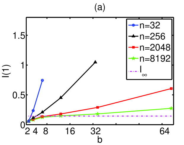
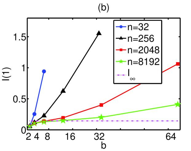
Figure 1: A. Papana

The MI for lag one $I(1)$ from the binning estimators ED and EP increases always with the number of bins $b$. Thus for white noise where $I_{\infty}(1)=0$ the best choice for $b$ is 2 that gives the smallest positive $I(1)$. For the linear processes, $I(1)$ decreases with the time series length $n$ for each $b$, as shown in Fig. 1 for the ED and EP estimates of $I(1)$ from an AR(1) process.
===============================================
Figure 1 *** To be placed here ***
===============================================
We note that for sufficiently large $b$, $I(1)$ converges with $n$ to the true value ${\cal I}(1)=I_{\infty}(1)$ given in (5). On the other hand, for small $b$, $I(1)$ underestimates $I_{\infty}(1)$ depending again on $n$. Thus the optimal $b$ that gives the smallest $dI_{c}(l)$ and estimates best $I_{\infty}(1)$ depends on $n$.

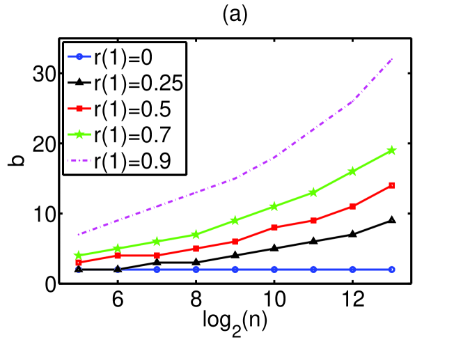
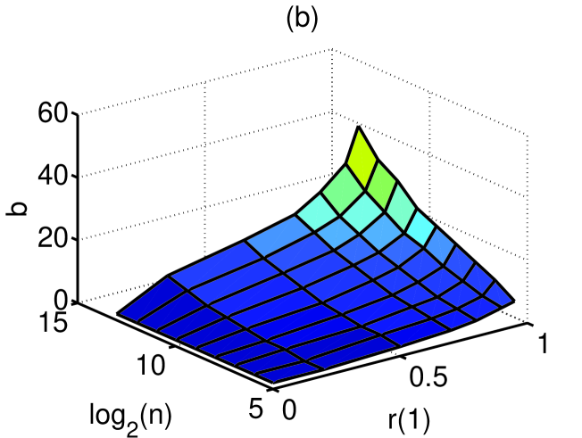
Figure 2: A. Papana

We have observed that $b$ depends also on the autocorrelation function $r(\tau)$ of the linear system. To investigate further this dependence we computed ED and EP estimates of $I(1)$ for a wide range of $r(1)$ values of an AR(1) process. We found that the optimal $b$ (found by the smallest $dI_{c}(l)$) increases smoothly with $n$ and $r(1)$, as shown in Fig. 2.
===============================================
Figure 2 *** To be placed here ***
===============================================
A search for a parametric fit of optimal $b$ regarding the graph of Fig. 2b resulted in the form

$$b=\alpha n^{\beta}e^{\gamma\rho^{2}}$$ (6)

where the coefficients $\alpha$, $\beta$, $\gamma$ take similar values for the ED and EP estimators (0.65,0.25,2.11 and 0.76,0.19,1.91 respectively).

Most of the criteria in Table 2 tend to overestimate $b$. To evaluate the performance of the 10 criteria in Table 2 and the proposed criterion in Eq.(6), we compute the total score $S_{c}$ of each criterion $c$, where $c=1,\ldots,11$, for all $L=126$ tested systems and time series lengths, as

$$S_{c}=\frac{\sum_{l=1}^{L}(\bar{I}_{c}(l)-I_{\infty}(l))^{2}}{\sum_{l=1}^{L}(\bar{\bar{I}}_{c}(l)-I_{\infty}(l))^{2}}$$ (7)

where for each case $l$, $\bar{\bar{I}}_{c}(l)=\frac{1}{11}\sum_{c=1}^{11}\bar{I}_{c}(l)$ is the grand mean of the means from all criteria. According to the score $S_{c}$, the proposed criterion in Eq.(6) for the optimal $b$, denoted H11, outperforms the other criteria when ED estimator is used, as shown in Table 4.
===============================================
Table 4 *** To be placed here ***
===============================================
For the EP estimator, criterion H9 scores lowest and H11 is ranked fifth but the differences in the scores of the best five criteria are comparatively small.

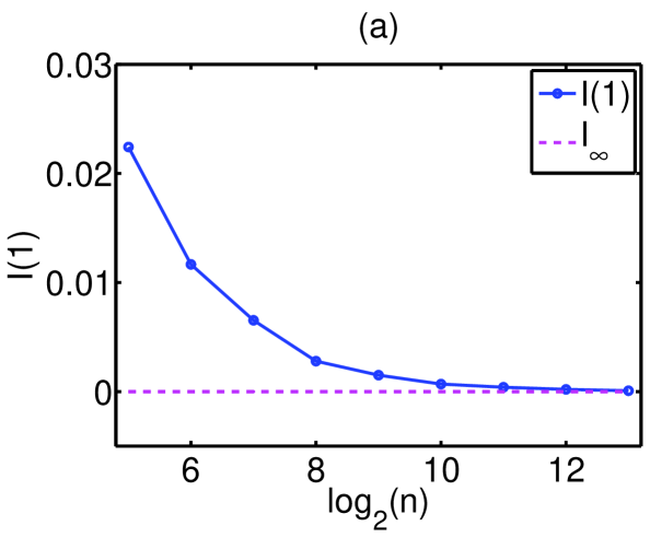
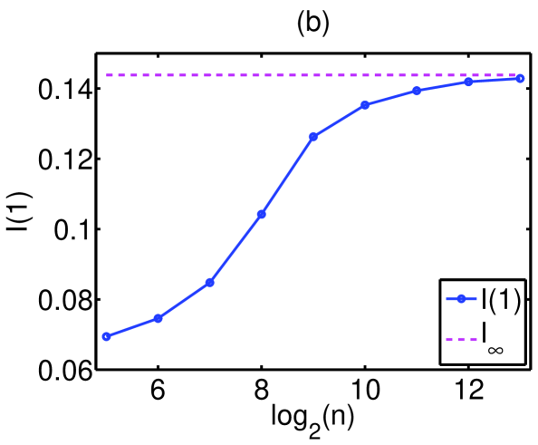
Figure 3: A. Papana

For certain bivariate distributions and Gaussian processes, it was found that the AD estimator was precise in estimating MI and converged fast to the true MI [Kraskov et al., 2004; Trappenberg et al., 2006]. We confirmed this result by our simulations on the white noise and linear systems with the remark that the convergence to $I_{\infty}$ is rather slow and is succeeded at large $n$, as shown in Fig. 3. ===============================================
Figure 3 *** To be placed here ***
===============================================

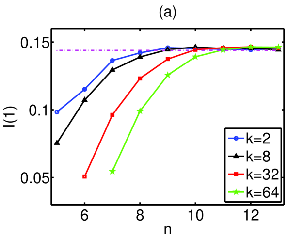
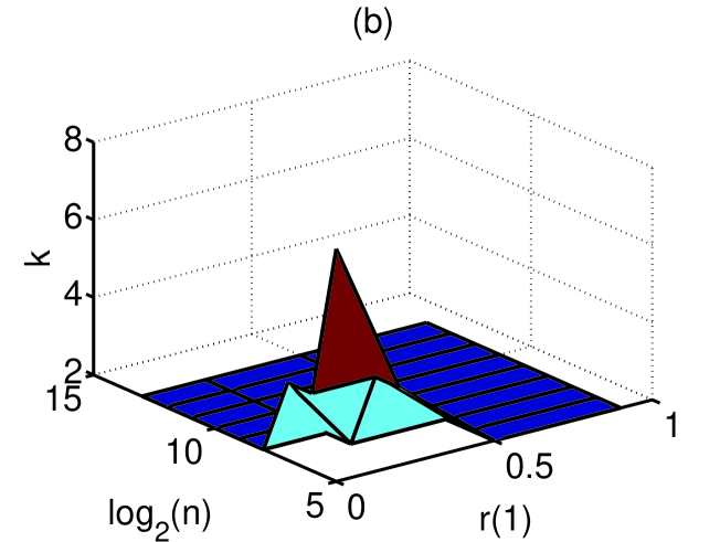
Figure 4: A. Papana

The number of nearest neighbors $k$ in the KNN estimator determines the roughness of approximation of the density functions in Eq.(1), which corresponds to the roughness of the partitioning in Eq.(2). The simulations showed that for white noise the MI estimated by KNN is close to zero for a long range of $k$ and the deviation from zero decreases as $k$ approaches $n/2$ (as reported also in [Kraskov et al., 2004]). For the linear systems the optimal $k$ is rather small. The dependence of the KNN estimator on $k$ holds mainly for small time series as for large $n$ the estimated MI converges to $I_{\infty}$ for any $k$, as shown in Fig. 4a.
===============================================
Figure 4 *** To be placed here ***
===============================================
Still, the convergence is slower for larger $k$. In any case, a highly accurate MI is attained with small $k$ for all but very small time series. For example, for an accuracy threshold of $10^{-4}$ in estimating $I_{\infty}$, i.e. $|I(1)-I_{\infty}|<10^{-4}$, the optimal choice for $k$ is 2 in almost all cases except for very small $n$ and $r(1)$, as shown in Fig. 4b. Note that even for white noise time series of small length, $k\leq 8$ reaches this accuracy threshold (the peak in the graph of Fig. 4b is for $n=2^{5}$ and $r(1)=0$).

For the two dimensional bandwidth $h_{2}$ we have considered $h_{2}=h_{1}$ and $h_{2}=\sqrt{2}h_{1}$ and studied the dependence of the estimated MI on $h_{1}$ and $h_{2}$ across a large range of bandwidths for white noise and linear systems. As for $k$ of the KNN estimator, MI converges with $n$ and faster for smaller $h_{1}$. For $h_{2}=h_{1}$ the convergence with $n$ is correctly towards $I_{\infty}$ (see Fig. 5a), but for $h_{2}=\sqrt{2}h_{1}$ MI decreases with $h_{1}$ and becomes negative (see Fig. 5b).
===============================================
Figure 5 *** To be placed here ***
===============================================

This result advocates the use of the same bandwidth for the kernel estimates of the marginal and joint distributions. We have also investigated whether there is dependence of $h_{1}$ on $r(1)$ and $n$. As for $k$ of the KNN estimator, there does not seem to be any systematic dependence. Using the same threshold accuracy in estimating $I_{\infty}$, the smallest optimal $h_{1}$ is always at a low level for all $r(1)$ and $n$ and there is no apparent pattern that would suggest a particular form of dependence of $h_{1}$ on $r(1)$ or $n$, as shown in Fig. 5c. The sudden jumps in the graph of Fig. 5c is due to numerical discrepancies around the chosen threshold for different $h_{1}$ values.

In order to evaluate the criteria for selecting $h_{1}$ and $h_{2}$ in Table 3, we computed for each criterion the score defined in Eq.(7) for all cases. The five optimal criteria and their scores for varying lengths of time series from white noise and linear systems are C1 ($0.85$), C3 ($0.94$), C2 ($0.96$), C4 ($1.57$) and C9 ($1.67$). The simplest criteria turned out to score lowest with best being the ”Gaussian” rule of Silverman C1 (see also Eq.(4)).

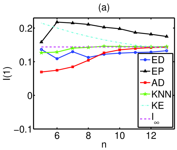
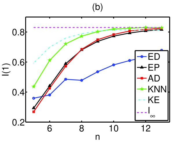
Figure 6: A. Papana

Summarizing the results on white noise and linear systems, it turns out that fixed binning estimators are the most dependent on the free parameter, the number of bins $b$, whereas for KNN and KE estimators a small number of neighbors $k$ and bandwidth $h_{1}$, respectively, turns out to be sufficient for all but very small time series length $n$ and weak autocorrelation $r(\tau)$. In such cases, binning estimators can approximate $I_{\infty}$ better with a relatively small $b$ and we provided an expression for this involving $n$ and $r(1)$. All estimators are consistent but converge at different rates to the true or asymptotic MI $I_{\infty}$, as shown in Fig. 6 for the AR(1) system with weak and strong autocorrelation.
===============================================
Figure 6 *** To be placed here ***
===============================================

In general, the KNN estimator converges fastest. To this respect, the parameter-free AD estimator would be the second best choice after the KNN estimator because it showed a slower convergence rate. KE estimator has about the same convergence rate as AD and is not significantly affected by parameter selection (for $h_{2}=h_{1}$), however it would not be preferred due to its computational cost. The estimation accuracy of each estimator is quantified by the index $dI_{c_{opt}}=\sum_{i=1}^{L}(\bar{I}_{c_{opt}}(l)-I_{\infty}(l))^{2}$, where $L=126$ and $c_{opt}$ is the optimal free parameter found in the simulations above, i.e. H11 for $b$ in ED and H9 for $b$ in EP, $k=2$ for KNN, and C1 for the bandwidths in KE. The smallest index $dI_{c_{opt}}=0.254$ was obtained by ED, followed by KE (0.302) and KNN (0.496), whereas AD and EP scored worse (1.865 and 2.231, respectively). Our numerical analysis on the linear systems and noise showed that for the three aspects of estimation considered, i.e. parameter dependence, rate of convergence, and accuracy of estimation, no estimator ranks first but KNN and KE turn out to perform overall best.

4.2 Results on nonlinear maps

In terms of chaotic systems, let us first note that MI can be viewed as a measure on the reconstructed attractor projected on $\Re^{2}$, i.e. on points $[x_{t},x_{t-\tau}]^{\prime}$. Due to the fractal structure in all scales of the chaotic attractor, ${\cal I}(\tau)$ defined in terms of a partition (see Eq.(2)) increases with finer partition towards the limit of ${\cal I}(\tau)$ given in Eq.(1) for the continuous space. On the other hand, for the estimation of entropy, and particularly the Kolmogorov-Sinai or metric entropy, it is postulated that there exists a so-called generation partition that gives the expected entropy value and further refinement to this partition does not increase further the computed entropy [Walter, 1975; Cohen & Procaccia, 1985]. However, with regard to the Shannon entropy, we observed that we can only get an upper limit of MI from the KNN estimator with $k=2$ as the estimation algorithm does not allow for a finer partition, whereas increasing $b$ for the binning estimators or decreasing $h_{1}$ for the KE estimator within the tested range does not seem to lead to convergence of MI.

The true ${\cal I}(\tau)$ in Eq.(1) is not known since the joint distribution of $[x_{t},x_{t-\tau}]^{\prime}$ is also not known. This prevents the direct comparison of the estimators and the search for optimal free parameters. The presence of noise in chaotic time series sets a limit to the scale where fractal details can be observed and consequently to the finiteness of the partition when estimating ${\cal I}(\tau)$. In that case, an asymptotic $I_{\infty}$ does exist and the performance of the estimators in terms of the free parameter and time series length can be compared, also for different noise levels. In the following, we try to delineate the differences among estimators in estimating $I_{\infty}$ and particularly in converging to $I_{\infty}$ with respect to the time series length and their free parameter.

The discussion above would suggest that the estimated MI should always increase as the partition gets finer, but in practice this requires a sufficient time series length $n$. For the binning estimators the optimal number of bins $b$, i.e. the $b$ giving largest MI and minimum $|I_{\infty}(\tau)-\bar{I}_{c}(\tau)|$, is not always the largest (limited to $b=64$ in our study) but increases with $n$, as shown in Fig. 7a for the ED estimator and the noise-free Henon map.
===============================================
Figure 7 *** To be placed here ***
===============================================
In the same figure the limits for optimal $b$ from the suggested criterion H11 in Eq.(6) (lower for r$(1)=0$ and upper for r$(1)=1$) are shown with dotted lines and are well beyond the optimal bins found for small lags. For this system, $I(\tau)$ decreases smoothly with $\tau$ and therefore the optimal $b$ decreases as well. For $\tau=10$, $I(\tau)$ levels off for small $n$ and then $b\simeq 2$ is optimal, but as $n$ increases more bins give indeed larger values of MI. Thus as $n$ increases weak MI for large $\tau$ becomes significant and can be distinguished from the plateau of independence only when a larger $b$ is used for the binning estimator. However, for a fixed $b$ MI converges to $I_{\infty}$ with $n$, even for noise-free data (Fig. 7c).

With the addition of noise, $I(\tau)$ decreases and the optimal number of bins drops, as shown in Fig. 7b and d respectively for $20\%$ additive noise on the Henon time series. The stronger the noise component is, the more the deterministic structure is masked and the faster the estimated MI levels towards zero with the lag. For the noisy chaotic data, the pattern of the dependence of the binning estimates of MI to $n$ and $b$ is closer to the one observed for the linear systems. For example, the range of optimal $b$ in Fig. 7b is at the level of $b$ given by the suggested criterion H11 for $r(1)$ ranging from 0 to 1. The results on EP estimator are similar.

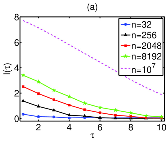
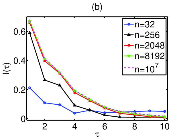
Figure 8: A. Papana

In line with the ED and EP estimators, the AD estimator does not converge with $n$ to $I_{\infty}$ for the nonlinear systems unless the fine partition is limited by the presence of noise, as shown in Fig. 8 for the Henon map.
===============================================
Figure 8 *** To be placed here ***
===============================================
The increase of $n$ directs the algorithm of AD to make a finer partition which results in a larger $I(\tau)$. The effect of $n$ on the adaptive estimator decreases with the increase of the noise level.

As pointed earlier, there is a loose relationship between the number of nearest neighbors $k$ in the KNN estimator and the number of bins $b$ in the binning estimators, i.e. small $k$ corresponds to large $b$. The lower limit $k=1$ corresponds to the finest partition for the given data, and the analogue $b$ could be formidably large and is not reached in our study as $b$ goes up to 64 (the same stands for $b$ up to 256). Thus direct comparison to binning estimators when $k$ is very small cannot be drawn. For noise-free chaotic time series, very fine partitions are sought and this agrees with the suggestion in Kraskov et al. [2004] to use small $k$ at the order of $3$, which was also used in other simulation studies [Kreuz et al., 2007; Khan et al., 2007]. In Fig. 9a, we show for the noise-free Henon map that ${\it I}(\tau)$ increases with decreasing $k$.
===============================================
Figure 9 *** To be placed here ***
===============================================
For small $n$, a large value of $k$ gives a poor estimation of the densities and consequently of ${\it I}(\tau)$. For a fixed $k$, MI increases with $n$ (see Fig. 9b). Assuming a fixed $k$ the effect of $n$ on the KNN estimator is large similarly to the effect of $n$ on the AD estimator as there in no convergence of MI with $n$, contrary to the fixed-bin estimators. In agreement to the binning estimators, the MI from the KNN estimator decreases with the noise level. Therefore the dependence of KNN estimator on $n$ is smaller and $I(\tau)$ converges faster to $I_{\infty}$ with $n$ (Fig. 9c). Further, for larger $n$ the estimation is the same regardless of the value of $k$.

The dependence of the KE estimator on the bandwidth $h_{1}$ is similar to the dependence of the KNN estimator on $k$. As shown in Fig. 10a and b for the noise-free Henon map, ${\it I}(\tau)$ increases with the decrease of $h_{1}$ ranging from 0.01 to 2.
===============================================
Figure 10 *** To be placed here ***
===============================================
We note that such extremely large values of ${\it I}(\tau)$ for very small bandwidth $h_{1}$ do not occur by any other estimator. Given that the KNN estimator for $k=1$ sets an upper limit for the estimated ${\it I}(\tau)$ on the given time series, larger ${\it I}(\tau)$ obtained by the KE estimator are superficially overflown estimates due to the use of an unsuitably small $h_{1}$ for the given time series. This systematic bias for very small $h_{1}$ is more pronounced with the addition of noise as it persists at the same level for larger $\tau$ (see Fig. 10c). For the noisy data, ${\it I}(\tau)$ decreases and differences with respect to the partitioning parameters are smaller, a feature we observed also with the other estimators (see Fig. 10c and d). Also, the estimated $I(\tau)$ is rather stable to the change of $n$.

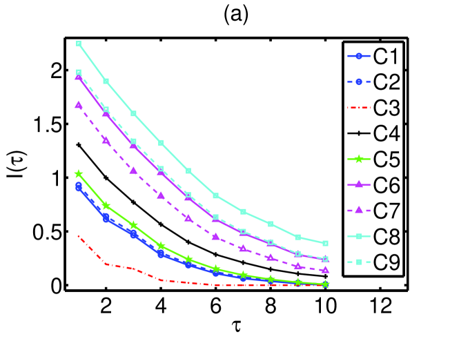
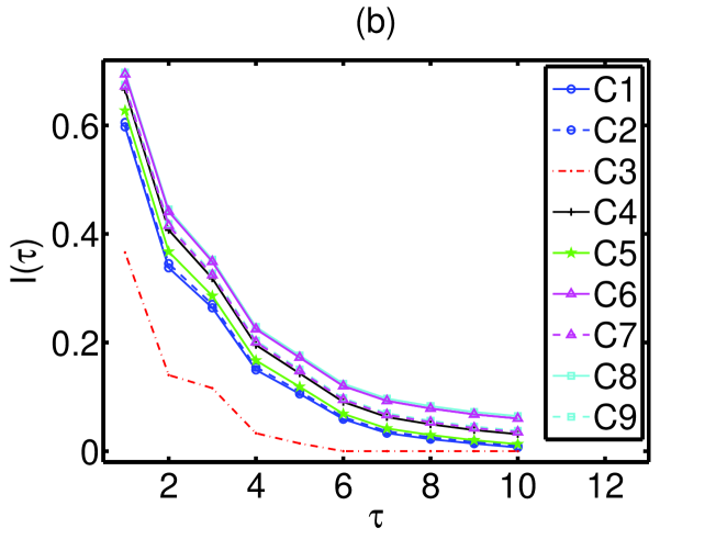
Figure 11: A. Papana

Regarding the $9$ criteria for selecting $h_{1}$ (and at cases $h_{2}$, see Table 3), the estimated bandwidths vary with the criterion but within a small range, e.g. for $n=256$ they are bounded in $[0.13,0.35]$ except C3 that always gives larger bandwidths and in this case $h_{1}\simeq 0.7$). Deviations of the estimated bandwidths hold for larger $n$ but at smaller magnitudes, e.g. for $n=8192$, they are bounded in $[0.03,0.18]$ and for C3 $h_{1}\simeq 0.37$). All criteria depend on $n$ in a similar way and estimate smaller bandwidths as $n$ increases giving larger ${\it I}(\tau)$ (see Fig. 11a for $n=8192$).
===============================================
Figure 11 *** To be placed here ***
===============================================
When noise is added to the time series, the estimated ${\it I}(\tau)$ using different bandwidth selection criteria converge and are rather stable to the change of $n$ (see Fig. 11b).

Contrary to linear systems, for noise-free nonlinear maps, the estimated MI does not converge to an asymptotic $I_{\infty}$ and even for very large time series the MI values computed by different estimators vary, as we tested for $n=10^{7}$. For increasing $n$, a finer partition gives larger MI regardless of the selected estimator. The closest approximation to the finest partition for a large $n$ is succeeded by the KNN estimator using a very small $k$, say $k=2$ for $n=10^{7}$. This turned out to be indeed an upper bound of the estimated MI for large $n$. For the other estimators, restrictions to the partition resolution, i.e. smallest $h_{1}$ for KE and largest $b$ for the binning estimators, bound the estimated MI to smaller values. For example, bins up to $b=256$ for ED and EP estimators underestimate MI for $n=10^{7}$, meaning that $b$ has to increase towards computationally prohibitive large magnitudes to succeed an adequately fine partition for this data size. In the same way, the bandwidth $h_{1}$ has to decrease accordingly with $n$ and for large $n$ the KE estimator turns out to be computationally ineffective. The presence of noise sets a lower limit to the partition resolution and allows for an asymptotic MI value $I_{\infty}$ to which all estimators converge with $n$ for suitably fine partition.

The results on the different estimators were only given for the Henon map in order to facilitate comparisons, but qualitatively similar results are obtained from the same simulations on the Ikeda map.

4.3 Results on nonlinear flows

When using MI on nonlinear flows the interest is often in extracting the lag $\tau_{0}$ of the first minimum of MI. We examine the estimate of $\tau_{0}$ with the different MI estimators on the Mackey-Glass system for delays $\Delta=17,30$ and $100$ that regard increasing complexity of correlation dimension being roughly 2,3 and 7, respectively [Grassberger & Procaccia, 1983].

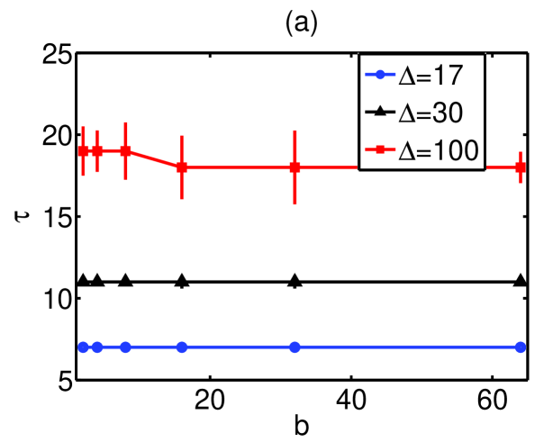
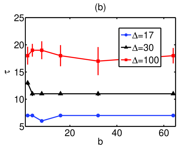
Figure 12: A. Papana

The simulations using the ED and EP estimators showed that the same $\tau_{0}$ is estimated for all $b$, all $n$ and noise levels, and for $\Delta=17$ and $\Delta=30$. For $\Delta=100$ we estimated the lag for which MI levels off and there was some variation in the selection of $\tau_{0}$ (see Fig. 12).
===============================================
Figure 12 *** To be placed here ***
===============================================
Although ${\it I}(\tau)$ increases with $b$, $\tau_{0}$ does not vary with $b$. Moreover, the estimate of $\tau_{0}$ is stable with $n$ and the addition of noise.

AD estimator is also not affected by $n$, when computing the lag of the minimum MI $\tau_{0}$ in the Mackey-Glass system (see Fig. 13a).
===============================================
Figure 13 *** To be placed here ***
===============================================
Addition of noise does not affect the mean $\tau_{0}$, as shown in Fig. 13b. From simulations on the Mackey-Glass system with $\Delta=100$ we observe that the mean estimated lag that MI levels off, holds for increasing $n$ (see Fig. 13c) and addition of noise does not affect it.

The estimation of $\tau_{0}$ using the KNN estimator on the Mackey Glass systems varies more with $n$ and $k$ than for the binning estimators, as shown in Fig. 14a and b.
===============================================
Figure 14 *** To be placed here ***
===============================================
With the addition of noise, the variance of the estimated $\tau_{0}$ decreases with respect to $k$, and the mean is rounded to the same integer for all $k$. For the Mackey Glass system with $\Delta=100$ we observed that there is consistency with $k$ and $n$, with MI for all $k$ having the same shape and therefore giving the same lag for levelling off (see Fig. 14c).

The mean estimated $\tau_{0}$ using the KE estimator on realizations of each of the three Mackey-Glass systems is stable against changes in the time series length and bandwidth as for the binning estimators.

Our simulations showed that all estimators identify sufficiently $\tau_{0}$ as the shape of the MI function is not affected significantly by $n$ or by the addition of noise. ED and KE estimators are the estimators of choice for this task, as they give smaller variation in the estimation of $\tau_{0}$ compared to the other estimators.

5 Discussion

MI estimators are sensitive to their free parameter, with binning estimators (ED and EP) being the most affected. There is a loose correspondence among the different free parameters $b$, $k$ and $h_{1}$ depending also on the time series length. Thus the differences in the performance of the estimators can be explained to some degree by the coarseness of the partition as determined by the free parameter. The choice of $b$ for the binning estimators determines the bin size of the partition. The analogue of the bin size for the KNN estimator is the size of neighborhoods given by the number of neighbors $k$ and for the KE estimator is the size of the efficient support of the kernel approximation given by the bandwidth $h_{1}$ (and $h_{2}$). The simulation results have quantified the correspondence of the different free parameters and showed that for large time series, a suitable refined partition can be easily accommodated by a very small $k$ or $h_{1}$, whereas for the binning estimators the requirement for a very large $b$ renders the binning estimator computationally ineffective. To this respect, the KNN estimator adapts easily to a refined partition by setting, say, $k=2$, as does the adaptive binning estimator (AD) that has no free parameter, whereas $h_{1}$ has to be further investigated at ranges of small values.

The optimization of the parameters of the estimators is very crucial, even more than the choice of the estimator. Therefore, we focused on estimating the optimal free parameter of each estimator in order to fairly evaluate the estimators. For linear systems, we evaluated also different selection criteria for the optimal free parameter and based on the simulation study we proposed for the fixed-binning estimators the optimal $b$ as a function of the autocorrelation and the time series length $n$. The parameter-free AD estimator tends to overestimate MI compared to the other estimators, indicating that the in-build partition algorithm of AD terminates at a very fine partition. The KNN estimator turns out to be the least sensitive to its free parameter. For example, $k=2$ that gives a very fine partition does not deviate much for smaller time series where larger $k$ are more appropriate. Our simulation results on the linear systems have shown that the KE estimator depends less than the binning estimators on the free parameter for the selected ranges of $h_{1}$ and $b$, respectively.

For noise-free nonlinear systems, all estimators lack consistency, i.e. the estimated MI does not converge with $n$ to an asymptotic value. Therefore, optimal parameter cannot be derived for these systems. The optimal parameter values found for the linear systems tend to give conservative estimates of MI for the nonlinear systems, for which a finer partition is required. This is accommodated by a small $k$ in the KNN estimator. Indeed the simulation study on the different chaotic systems has shown that the KNN estimator has the least variance with the free parameter $k$ than all other estimators. For noisy nonlinear systems, the MI from all estimators converge with $n$ to an upper limit set by noise and KNN estimator for $k=2$ turned out to reach this limit faster.

For the computation of the lag $\tau_{0}$ of the first minimum of MI, the binning estimators ED and EP as well as the KE estimator seem to perform best. For the Mackey-Glass system, we observed that although $I(\tau)$ may vary with the free parameter of the estimator and $n$, $\tau_{0}$ is rather stable. The addition of noise does not seem to effect the estimation of $\tau_{0}$.

The KE estimator has the highest computational cost and the fixed-binning estimators become computationally intractable when $b$ has to be very large, as for long chaotic time series. On the other hand, the KNN estimator is rather fast for long time series that require small $k$ for which neighbor search is faster. The computation efficiency of the AD estimator is comparable to that of KNN and these two estimators seem to be the most appropriate for all practical purposes in terms of computational efficiency, parameter selection (small $k$ for KNN and no free parameter for AD) and accuracy of estimation (with KNN scoring better than AD).

We note that the consistency of estimators of MI on linear systems is not indicative of the behavior of the estimators on nonlinear systems. Although consistency of estimators is claimed in some recent works, this might be due to the use of only linear systems or noisy real data, such as EEG.

6 Acknowledgments

This research project is implemented within the framework of the ”Reinforcement Programme of Human Research Manpower” (PENED) and is co-financed at $90\%$ jointly by E.U.-European Social Fund ($75\%$) and the Greek Ministry of Development-GSRT ($25\%$) and at $10\%$ by Rikshospitalet, Norway.

Table 1: The simulation systems and their parameters. The input white noise for the linear systems (rows 4 to 7) and the observational white noise for the nonlinear systems (rows 8 to 10) have zero mean and standard deviation one. Gamma noise is skewed with $\gamma=0.5$.The parameter notations are $\mu$ for the mean, $\sigma$ for the standard deviation and $\gamma$ for the skewness coefficient, $\varphi$ for the coefficient of the autoregressive part for AR(1) and ARMA(1,1) and $\vartheta$ for the coefficient of the moving average part of ARMA(1,1), $\tau_{s}$ for the sampling time and $\delta$ for the discretization time for the Mackey-Glass system. The noise levels considered for the nonlinear systems are $20\%$ and $40\%$.

Systems	Parameters	Noise
Gaussian white noise	$\mu=0,\sigma=1$
Gamma white noise	$\mu=0,\sigma=1,\gamma=0.5$
AR(1)	$\varphi=0.5,0.9,-0.5,-0.9$	Gaussian
AR(1)	$\varphi=0.5,0.9,-0.5,-0.9$	Gamma
ARMA(1,1)	$\varphi=0.9,\vartheta=0.6$ & $\varphi=0.7,\vartheta=0.3$	Gaussian
ARMA(1,1)	$\varphi=0.7,\vartheta=0.3$ & $\varphi=0.3,\vartheta=0.1$	Gamma
Henon	$a=1.4,b=0.3$	Gaussian
Ikeda	$a=1.0,b=0.9,\kappa=0.4,\eta=6.0$	Gaussian
Mackey-Glass	$\Delta=17,30,100$, $\tau_{s}=17$, $\delta=0.1$	Gaussian

Table 2: Criteria for the selection of the number of bins. The parameters in the expressions are the time series length $n$, the standard deviation $s$, the interquartile range IQR, the range of the data $R$ and the standardized skewness $\gamma_{2}$ as defined in [Doane, 1976]. The exact expressions for criteria H8 and H9 can be found in the in the corresponding references, given in the third column.

. Criteria Number of bins Reference H1 $1+\log_{2}{n}$ [Sturge, 1926] H2 $1.87(n-1)^{0.4}$ [Bendat & Piersol, 1966] H3 $1+\log_{2}{n}+\log_{2}\gamma_{2}$ [Doane, 1976] H4 $\sqrt{n}$ [Tukey & Mosteller, 1977] H5 $\frac{Rn^{1/3}}{3.49s}$ [Scott, 1979] H6 $\frac{Rn^{1/3}}{{2(IQR)}}$ [Freedman & Diaconis, 1981] H7 $\sqrt[3]{2n}$ [Terrell & Scott, 1985] H8 min. of stochastic complexity [Rissanen, 1992] H9 mode of log of marginal posterior pdf [Knuth, 2006] H10 $\sqrt{n/5}$ [Cochran, 1954]

Table 3: Criteria for the selection of bandwidths for one ($h_{1}$) and two ($h_{2}$) dimensions. The parameters in the expressions are $a=1.8-r(1)$ if $n<200$ and $a=1.5$ if $n\geq 200$, where $r(1)$ is the autocorrelation at lag $1$, $R=1/2{\sqrt{\pi}}$, $s$ is the standard deviation and IQR is the interquartile range of the data. The exact expressions for the last four criteria can be found in the corresponding references, given in the third column.

Criteria	$h_{1}$	$h_{2}$	Reference
C1	$(4/3n)^{1/5}$	$(1/n)^{1/6}$	[Silverman, 1986]
C2	$(4/3n)^{1/5}$	$(4/5n)^{1/6}$	[Silverman, 1986]
C3	$1.06an^{-1/5}$	$an^{-1/6}$	[Harrold et al., 2001]
C4		$h_{1}$	[Silverman, 1986]
C5	$(\frac{8{\sqrt{\pi}}R}{3n})^{1/5}\min(s,\frac{\mbox{IQR}}{1.349})$	$\sqrt{2}h_{1}$	[Wand & Jones, 1995]
C6		$h_{1}$
C7	L-stage direct plug-in	$\sqrt{2}h_{1}$	[Wand & Jones, 1995]
C8		$h_{1}$
C9	Solve-the-equation plug-in	$\sqrt{2}h_{1}$	[Sheather & Jones, 1991]

Table 4: Ranking and score $S$ of the $5$ criteria for $b$ scoring lowest for the ED and EP estimators for varying lengths of time series from white noise and linear systems.

Criteria	$S$ for ED	Criteria	$S$ for EP
H11	0.25	H9	0.61
H7	0.94	H7	0.62
H8	1.16	H8	0.65
H5	1.20	H10	0.67
H9	1.41	H11	0.72

Figures captions

Figure 1: Mean $I(1)$ as a function of $b$ from 1000 realizations of AR(1) with coefficient $\varphi=r(1)=0.5$ and additive Gaussian noise for (a) the ED and (b) the EP estimator and for data sizes as given in the legend.

Figure 2: (a) Optimal number of bins for different $n$ for AR(1) systems with lag one autocorrelation $r(1)$ as in the legend. (b) Graph of the optimal $b$ for a range of $\log_{2}(n)$ and $r(1)$. The results in both panels regard the ED estimator.

Figure 3: Mean estimated MI with AD estimator as a function of $n$ from 1000 realizations of (a) normal white noise and (b) AR(1), with $r=0.5$ and normal input white noise.

Figure 4: (a) Mean estimated MI with the KNN estimator as a function of $n$ from 1000 realizations of AR(1) with $r(1)=0.5$ and normal input white noise for $k$ as in the legend. The dotted line stands for $I_{\infty}$. (b) Graph of the optimal $k$ for a range of $\log_{2}(n)$ and $r(1)$.

Figure 5: Mean estimated MI with the KE estimator as a function of $h_{1}$ from 1000 realizations of $AR(1)$ with $r(1)=0.5$ and normal input white noise for (a) $h_{1}=h_{2}$, and (b) $h_{1}=\sqrt{2}{h_{2}}$, and $n$ as in the legend. (c) Graph of the optimal $h_{1}$ for a range of $\log_{2}(n)$ and $r(1)$.

Figure 6: (a) Mean estimated MI vs $n$ for the estimators given in the legend from simulations on AR(1) with $r(1)=0.5$ and normal input white noise. For each estimator the optimal free parameter is considered, i.e. H11 for ED, H9 for EP, $k=2$ for KNN and C1 for KE. (b) As (a) but for $r(1)=0.9$.

Figure 7: (a) Optimal number of bins $b$ as a function of the time series length $n$ for the ED estimator from 1000 realizations of the Henon map for different lags, as given in the legend. (b) Same graph as in (a) but for the Henon map with $20\%$ additive noise. In both plots the dotted lines give the optimal number of bins $b$ from the suggested criterion in (6) assuming r(1)=0 and r(1)=1, as given in the plot. (c) Mean estimated MI with ED estimator as a function of $\tau$ from 1000 realizations of the Henon map for $b=32$, and $n$ as in the legend. (d) As (c) but for Henon map with $20\%$ additive noise.

Figure 8: Mean estimated MI with AD estimator as a function of $\tau$ from 1000 realizations of the Henon map with no noise in (a) and with $20\%$ noise in (b).

Figure 9: (a) Mean estimated MI with KNN estimator as a function of $\tau$ from $1000$ realizations of the Henon map, for $n=256$ and $k$ as in the legend. (b) As in (a) but for $k=2$ and $n$ as in the legend. (c) As in (a) but for Henon map with $20\%$ additive noise.

Figure 10: (a) Mean estimated MI with KE estimator as a function of $\tau$ from $1000$ realizations of the Henon map, for $n=512$ and bandwidths as in the legend. (b) As in (a) but for $n=4096$ and bandwidths as in the legend. (c) and (d) are the same as (a) and (b) respectively but for the Henon map with $20\%$ additive noise.

Figure 11: (a) Mean estimated MI with KE estimator as a function of $\tau$ from $1000$ realizations of the noise-free Henon map with $n=8192$ and nine bandwidth selection criteria as given in the legend. (b) As (a) but for $20\%$ additive noise.

Figure 12: (a) Mean estimated $\tau_{0}$ and standard deviation as error bar as a function of $b$ from all time series lengths using the ED estimator on the Mackey-Glass system with $\Delta=17,30,100$, as given in the legend. (b) As in (a) but for the EP estimator.

Figure 13: (a) Mean estimated $\tau_{0}$ and standard deviation as error bar as a function of $n$ using the AD estimator on 1000 realizations of the Mackey-Glass system with $\Delta=17,30$, as given in the legend. (b) As in (a) (without standard deviations) for additive noise with levels $20,40\%$, as given in the legend. (c) Mean estimated MI with the AD estimator as a function of $\tau$ from 1000 realizations of the Mackey-Glass with $\Delta=100$, for $n$ as in the legend.

Figure 14: Mean estimated $\tau_{0}$ as a function of $n$ using the KNN estimator on 1000 realizations of the Mackey-Glass system with (a) $\Delta=17$, and (b) $\Delta=30$. (c) Mean estimated MI with the KNN estimator as a function of $\tau$ from 1000 realizations of the Mackey-Glass with $\Delta=100$, for $k$ as in the legend and $n=2048$.

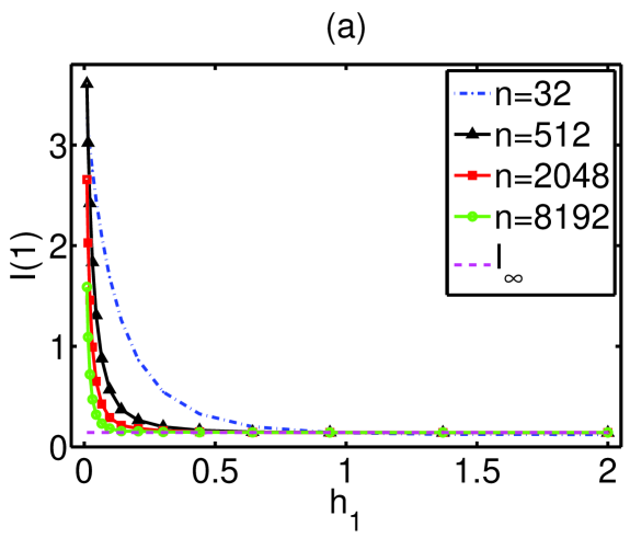
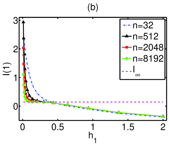
Figure 5: A. Papana

Figure 5c: A. Papana

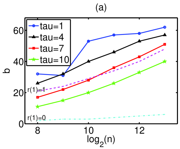
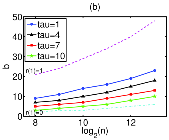
Figure 7: A. Papana

Figure 7c and d: A. Papana

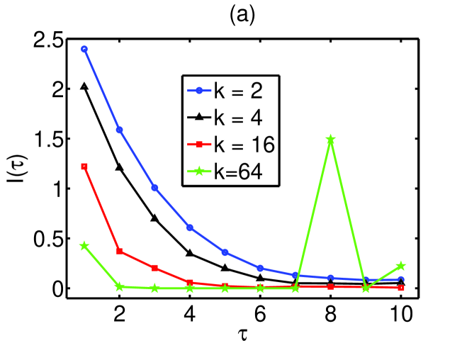
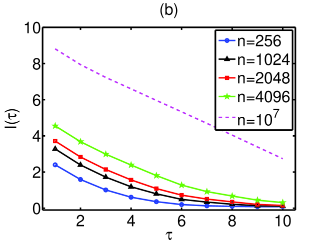
Figure 9: A. Papana

Figure 9c: A. Papana

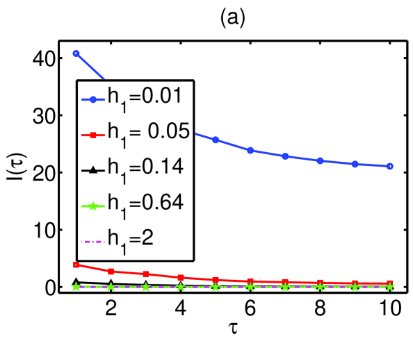
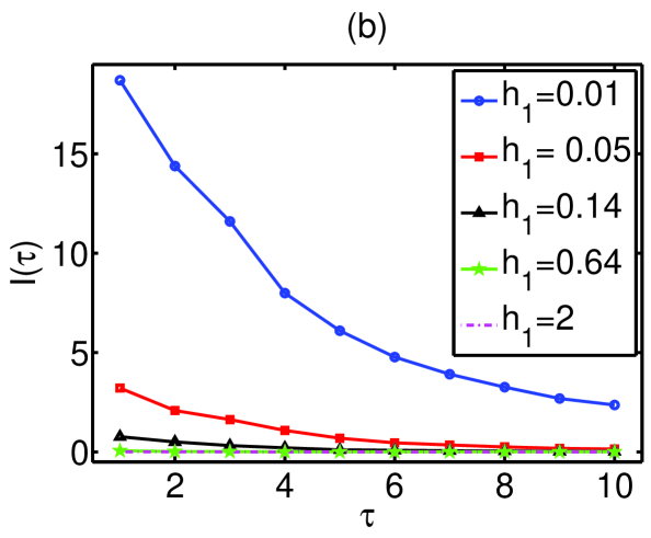
Figure 10: A. Papana

Figure 10c and d: A. Papana

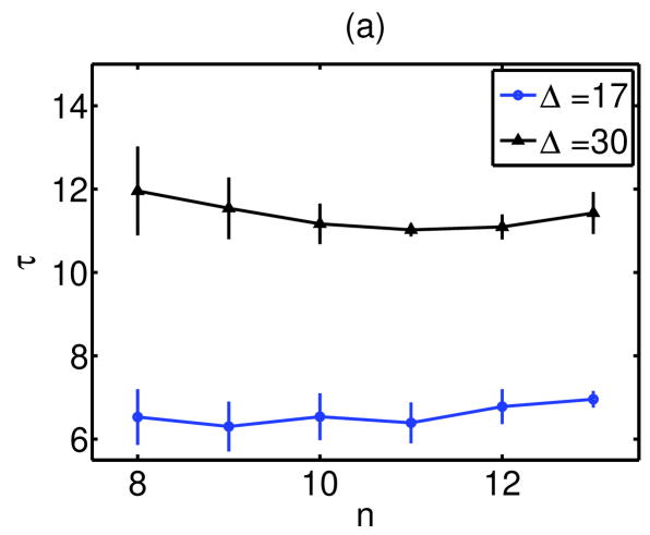
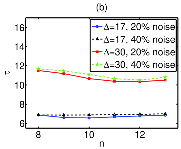
Figure 13: A. Papana

Figure 13c: A. Papana

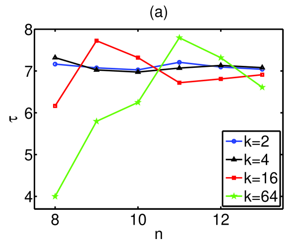
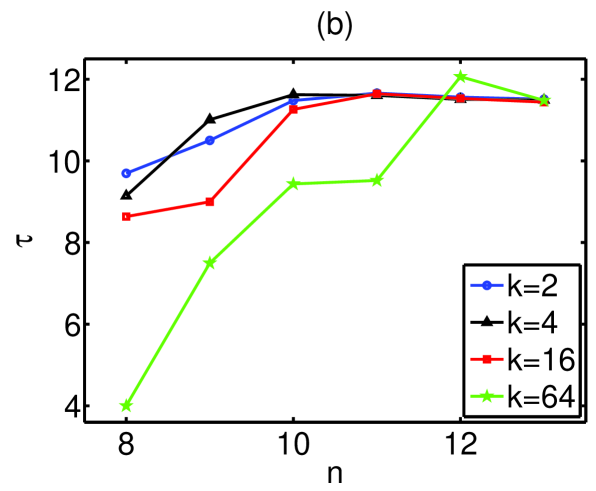
Figure 14: A. Papana

Figure 14c: A. Papana

References

- Abarbanel et al. [2001] Abarbanel, H., Masuda, N., Rabinovich, M. & Tumer, E. [2001] ”Distribution of mutual information,” Phys. Lett. A 281(5-6), 368 -373.
- Bendat & Piersol [1966] Bendat, S. & Piersol, A. [1966] Measurements and Analysis of Random Data (John Wiley and Sons, New York).
- Blinnikov & Moessner [1998] Blinnikov, S. & Moessner, R. [1998] ”Expansions for nearly Gaussian distributions,” Astron. Astrophys. Sup. 130(1), 193–205.
- Bonnlander & Weigend [1994] Bonnlander, B. & Weigend, A. [1994] ”Selecting input variables using mutual information and nonparametric density estimation,” In Proc. of the 1994 Int. Symp. on Artificial Neural Networks (ISANN ’94), Taiwan, pp. 42–50.
- Cellucci et al. [2005] Cellucci, C., Albano, A. & Rapp, P. [2005] ”Statistical validation of mutual information calculations: Comparison of alternative numerical algorithms,” Phys. Rev. E 71, 066208.
- Cochran [1954] Cochran, W. [1954] ”Some methods for strengthening the common X2 tests,” Biometrics 10(4), 417–451.
- Cohen & Procaccia [1985] Cohen, A. & Procaccia, I. [1985] ”Computing the kolmogorov entropyfrom time signals of dissipative and conservative dynamical systems,” Phys. Rev. A 31(3), 1872–1882.
- Darbellay & Vajda [1999] Darbellay, G. & Vajda, I. [1999] ”Estimation of the information by an adaptive partitioning of the observation space,” IEEE T. Inform. Theory 45(4), 1315–1321.
- Daub et al. [2004] Daub, C., Steuer, R., Selbig, J. & Kloska, S. [2004] ”Estimating mutual information using B-spline functions: An improved similarity measure for analysing gene expression data,” Bioinformatics 5(1), 118.
- Diks & Manzan [2002] Diks, C. & Manzan, S. [2002] ”Tests for serial independence and linearity based on correlation integrals,” Stud. Nonlinear Dyn. E. 6(2), 1005.
- Diks & Panchenko [2008] Diks, C. & Panchenko, V. [2008] ”Rank-based entropy tests for serial independence,” Stud. Nonlinear Dyn. E. 12(1).
- Doane [1976] Doane, D. [1976] ”Aesthetic frequency classifications,” Am. Stat. 30(4), 181–183.
- Fraser & Swinney [1986] Fraser, A. & Swinney, H. [1986] ”Independent coordinates for strange attractors from mutual information,” Phys. Rev. A 33, 1134–1140.
- Freedman & Diaconis [1981] Freedman, D. & Diaconis, P. [1981] ”On the histogram as a density estimator: L2 theory,” Z. Wahrscheinlichkeit. 57, 453–476.
- Grassberger & Procaccia [1983] Grassberger, P. & Procaccia, I. [1983] ”Measuring the strangeness of strange attractor,” Physica D 9(1–2), 189–208.
- Grassberger [1988] Grassberger, P. [1988] ”Finite sample corrections to entropy and dimension estimates,” Phys. Lett. A 128(6–7), 369–373.
- Harrold et al. [2001] Harrold, T., Sharma, A. & Sheather, S. [2001] ”Selection of a kernel bandwidth for measuring dependence in hydrologic time series using the mutual information criterion,” Stoch. Env. Res. Risk A. 15(4), 310–324.
- Henon [1976] Henon, M. [1976] ”A two dimensional mapping with a strange attractor,” Commun. Math. Phys. 50(1), 69–77.
- Hively et al. [2000] Hively, L., Protopopescu, V. & Gailey, P. [2000] ”Timely detection of dynamical change in scalp EEG signals,” Chaos 10(4), 864–875.
- Hutter & Zaffalon [2005] Hutter, M. & Zaffalon, M. [2005] ”Distribution of mutual information from complete and incomplete data,” Comput. Stat. Data An. 48(3), 633–657.
- Ikeda et al. [1980] Ikeda, K., Kondo, K. & Akimoto, O. [1980] ”Optical turbulence: Chaotic behaviour of transmitted light from a ring cavity,” Phys. Rev. Lett. 45(9), 709- 712.
- Jones et al. [1996] Jones, M., Marron, J. & Sheather, S. [1996] ”A brief survey of bandwidth selection for density estimation,” J. Amer. Statist. Assoc. 91(433), 401 -407.
- Kantz & Schreiber [1997] Kantz, H. & Schreiber, T. [1997] Nonlinear Time Series Analysis. (Cambridge University Press, Reading, Massachusetts).
- Kantz & Shürmann [1996] Kantz, H. & Shürmann, T. [1996] ”Enlarged scaling ranges in entropy and dimension estimates,” Chaos 6(2), 167–171.
- Khan et al. [2007] Khan, S., Bandyooadhyay, S., Ganguly, A., Saigal, S., Erickson, D., Protopopescu, V. & Ostrouchov, G. [2007] ”Relative performance of mutual information estimation methods for quantifying the dependence among short and noisy data,” Phys. Rev. E 76(2), 026209.
- Knuth [2006] Knuth, K. [2006] ”Optimal data-based binning for histograms,” url: http://arxiv.org/abs/physics/0605197v1.
- Kraskov et al. [2004] Kraskov, A., Stögbauer, H. & Grassberger, P. [2004] ”Estimating mutual information,” Phys. Rev. E 69(6), 066138.
- Kreuz et al. [2007] Kreuz, T., Mormann, F., Andrzejak, R., Kraskov, A., Lehnertz, K., & Grassberger, P. [2007] ”Measuring synchronization in coupled model systems: A comparison of different approaches,” Physica D 225(1), 29- 42.
- Mackey & Glass [1977] Mackey, M. & Glass, L. [1977] ”Oscillation and chaos in physiological control systems,” Science 197, 287–289.
- Micheas & Zografos [2006] Micheas, A. & Zografos, K. [2006] ”Measuring stochastic dependence using -divergence,” J. Multivariate Anal. 97(3), 765–784.
- Moddemeijer [1989] Moddemeijer, R. [1989] ”On estimation of entropy and mutual information of continuous distributions,” Signal Process. 16(3), 233–248.
- Moon et al. [1995] Moon, Y., Rajagopalan, B. & Lall, U. [1995] ”Estimation of mutual information using kernel density estimators,” Phys. Rev. E 52(3), 2318–2321.
- Naa et al. [2002] Naa, S., Jina, S.-H., Kima, S. & Hamb, B.-J. [2002] ”EEG in schizophrenic patients: Mutual information analysis,” Clin. Neurophysiol. 113(12), 1954–1960.
- Nicolaou & Nasuto [2005] Nicolaou, N. & Nasuto, S. [2005] ”Mutual information for EEG analysis,” in Proc. 4th IEEE EMBSS UKRI Postgraduate Conference on Adv. in Biomed. Eng. and Med. Phys. (PGBIOMED’05) (Reading, UK) pp. 23–24.
- Palus [1993] Palus, M. [1993] ”Identifying and quantifying chaos by using information-theoretic functionals,” in Time Series Prediction: Forecasting the Future and Understanding the Past, Vol. XV of Santa Fe Institute Studies in the Sciences of Complexity, eds. Weigend, A. & Gershenfeld, N. (Addison-Wesley, Reading) pp. 387–413.
- Palus [1995] Palus, M. [1995] ”Testing for nonlinearity using redundancies: Quantitative and qualitative aspects,” Physica D 80(1), 186–205.
- Paninski [2003] Paninski, L. [2003] ”Estimation of entropy and mutual information,” Neural Comput. 15(6), 1191–1253.
- Pardo [1995] Pardo, J. [1995] ”Some applications of the useful mutual information,” Appl. Math. Comput., 72(1):33–50.
- Priness et al. [2007] Priness, I., Maimon, O. & Ben-Gal, I. [2007] ”Evaluation of gene-expression clustering via mutual information distance measure,” Bioinformatics 8(6), 111.
- Rissanen [1992] Rissanen, J. [1992] Stochastic Complexity in Statistical Inquiry (World Scientific, Singapore).
- Roulston [1997] Roulston, M. [1997] ”Significance testing of information theoretic functionals,” Physica D 110(1–2), 62–66.
- Schmid et al. [2004] Schmid, M., Conforto, S., Bibbo, D., & D’Alessio, T. [2004] ”Respiration and postural sway: Detection of phase synchronizations and interactions,” Hum. Movement Sci. 23(2), 105–119.
- Scott [1979] Scott, D. [1979] ’On optimal and data-based histograms,” Biometrika 66(3), 605–610.
- Sheather & Jones [1991] Sheather, S. & Jones, M. [1991] ”A reliable data-based bandwidth selection method for kernel density estimation,” J. Roy. Stat. Soc. B 53(3), 683–690.
- Silverman [1986] Silverman, B. [1986] Density Estimation for Statistics and Data Analysis (Chapman and Hall, London).
- Steuer et al. [2002] Steuer, R., Kurths, J., Daub, C., Weise, J. & Selbig, J. [2002] ”The mutual information: Detecting and evaluating dependences between variables,” Bioinformatics 18(2), S231–S240.
- Sturge [1926] Sturge, H. [1926] ”The choice of a class interval,” J. Am. Stat. Assoc. 21(1), 65–66.
- Terrell & Scott [1985] Terrell, G. & Scott, D. [1985] ”Oversmooth nonparametric density estimates,” J. Am. Stat. Assoc. 80, 209–214.
- Tourassi et al. [2001] Tourassi, G., Frederick, E., Markey, M. & Floyd, C. [2001] ”Application of the mutual information criterion for feature selection in computer-aided diagnosis,” Med. Phys. 28(12), 2394–2402.
- Trappenberg et al. [2006] Trappenberg, T., Ouyang, J. & Back, A. [2006] ”Input variable selection: Mutual information and linear mixing measures,” IEEE T. Knowl. Data Eng. 18(1), 37–46.
- Treves & Panzeri [1995] Treves, A. & Panzeri, S. [1995] ”The upward bias in measures of information derived from limited data samples,” Neural Comput. 7(2), 399–407.
- Tukey & Mosteller [1977] Tukey, J. & Mosteller, F. [1977] Data Analysis and Regression (Addison-Wesley, Reading, MA).
- Walter [1975] Walter, P. [1975] Ergodic Theory - Introductory Lectures Notes (Springer, Berlin).
- Wand & Jones [1993] Wand, M. & Jones, M. [1993] ”Comparison of smoothing parameterizations in bivariate kernel density estimation,” J. Am. Stat. Assoc. 88(422), 520–528.
- Wand & Jones [1995] Wand, M. & Jones, M. [1995] Kernel Smoothing (Chapman and Hall, London).
- Wicks et al. [2007] Wicks, R., Chapman, S. & Dendy, R. [2007] ”Mutual information as a tool for identifying phase transitions in dynamical complex systems with limited data,” Phys. Rev. E 75(5), 051125.