Capacitance measurements and electrostatic calibrations in experiments measuring the Casimir force

Abstract

We compare the results of capacitance measurements in the lens-plane and sphere-plane configurations with theoretical predictions from various models of a spherical surface. It is shown that capacitance measurements are incapable of discriminating between models of perfect and modified spherical surfaces in an experiment demonstrating the anomalous scaling law for the electric force. Claims to the contrary in the recent literature are explained by the use of irregular comparison. The data from capacitance measurements in an experiment measuring the Casimir force using a micromechanical torsional oscillator are shown to be in excellent agreement with theoretical predictions using the model of a perfect spherical surface.

I Introduction

Starting from 1997, measurements of the Casimir force 1 between a closely spaced gold coated spherical lens or sphere and a plate has attracted widespread attention in areas ranging from nanotechnology to constraining predictions of fundamental physical theories beyond the Standard Model (see Refs.  2 ; Book for a detailed analysis of all performed experiments). An important constituent of any Casimir force measurement is the electrostatic calibration. This allows an independent determination of some vitally important parameters (the absolute separation between two closely spaced bodies, the residual potential difference between their surfaces, spring constant etc.) by fitting the electric force arising between a lens or a sphere and a plate under an applied voltage to the known force law. The experimental procedures for electrostatic calibrations were discussed in detail in the pioneering papers (see, e.g., 2b ; 3 ; 4 ). A basic assumption used was that the electric force is given by the exact formula of electrostatics obtained for an ideal metal sphere above an ideal metal plane 5 . A very precise asymptotic expansion of this formula in powers of $(d/R)^{k}$ was also obtained 6 , where $k=-1,\,0,\,1,\,\ldots,\,6$, $d$ is the sphere-plate separation, and $R$ is the sphere radius. The first term of the expansion which is of order $R/d$ coincides with the electric force, as calculated by using the proximity force approximation (PFA) 7 . It is important to bear in mind that the typical sphere radii used in these experiments were about $100\,\mu$m and separation distances between the sphere and the plate were of order 100 nm 2 .

Reference 8 reconsidered electrostatic calibration in the sphere-plane geometry by replacing the small sphere with a spherical lens of centimeter-size radius $R$ at a very close separation from the plate, $d\geq 30\,$nm. Both test bodies were covered with gold layers. The experimental data obtained from the electrostatic calibration demonstrated an anomalous dependence of the gradient of the electric force on separation $\sim R/d^{1.7}$ instead of $R/d^{2}$, as follows from the main contribution to the exact formula mentioned above. This result was discussed in Refs. 9 ; 10 . Specifically, in Ref. 9 it was demonstrated that their data for the electrostatic force between a sphere and a plate in the separation range $d\geq 100\,$nm followed the standard electrostatic law. It was concluded 9 that the observation of Ref. 8 is not universal. In Ref. 10 a model of a modified geometry of a spherical surface was proposed which provides possible explanation for the anomalous behavior of the electric force observed in Ref. 8 . However, Ref. 11 refuted the explanation of the anomaly using the proposed model. According to Ref. 11 , this model, which explains the anomalous behavior of the gradient of electric force, “is hard to reconcile with the measurement of the capacitance versus distance that better follows the behavior expected for a sphere with a single radius of curvature”.

Taking into account that the possible reasons for the above-discussed anomaly are of major importance for all applications of the Casimir force, including constraining the Yukawa-type corrections to Newtonian gravity, we devote this paper to the capacitance measurements in the electrostatic calibration of the Casimir setup. In Sec. II a brief summary of the main results for the capacitance in the sphere-plane geometry is presented. These results are used in the following sections. In Sec. III the capacitance measurements of Ref. 11 (see also Ref. 12 ) are compared with theoretical predictions following from the model of a perfect spherical surface used in 11 ; 12 , and from the model with a modified surface 10 providing the explanation of the anomalous behavior of the elecric force 8 . We show that the conclusion of Ref. 11 , that the capacitance measurements are compatible with the model of perfect sphere, but incompatible with the model of modified spherical surface, is based on an irregular comparison. The point is that instead of the precise analytical expression for the capacitance following from the results of Ref. 10 , an inexact approximate representation for it was used in Ref. 11 to fit the experimental data. Section IV is devoted to the capacitance measurements in the experiment on the dynamic determination of the Casimir pressure by means of a micromechanical torsional oscillator. We present the experimental data for the capacitance in the configuration of a small Au-coated sapphire sphere above an Au-coated polisilicon plate, and demonstrate excellent agreement with theoretical results of electrostatics for a sphere-plane configuration with a perfectly shaped sphere. Section V contains our conclusions and discussion.

II Capacitance in a sphere-plate geometry

We consider an ideal metal sphere of radius $R$ at a close separation $d$ above an ideal metal plane. The exact expression for the electrical capacitance in such a configuration is given by 13

$$C(d)=4\pi\epsilon_{0}R\,{\rm sinh}\,\alpha\sum_{n=1}^{\infty}\frac{1}{{\rm sinh}(n\alpha)},$$ (1)

where ${\rm cosh}\,\alpha=1+d/R$ and $\epsilon_{0}$ is the permittivity of a vacuum. When a voltage $V$ is applied to the plane while the sphere is kept grounded, the electrostatic energy of sphere-plane interaction is given by

$$E(d)=-\frac{1}{2}C(d)(V-V_{0})^{2},$$ (2)

where $V_{0}$ is the residual potential difference when both bodies are grounded. Using Eq. (1) one obtains the exact expression for the electric force acting between a sphere and a plane 5

$$F(d)=-\frac{\partial E}{\partial d}=\frac{1}{2}(V-V_{0})^{2}\,\frac{\partial C(d)}{\partial d}$$ (3)

$$~{}~{}~{}~{}~{}=2\pi\epsilon_{0}(V-V_{0})^{2}\sum_{n=1}^{\infty}\frac{{\rm coth}\,\alpha-n{\rm coth}(n\alpha)}{{\rm sinh}(n\alpha)}.$$

In the limiting case of small separations, $d/R\ll 1$, an approximate expression for the capacitance (1) was obtained in Ref. 14

$$C(d)\approx 2\pi\epsilon_{0}R\left(\ln\frac{R}{d}+\ln\,2+\frac{23}{20}+\frac{\theta}{63}\right),$$ (4)

where $0\leq\theta\leq 1$.

In Ref. 6 a very precise expansion for the electric force (3) within a wide region of parameters was obtained in the form of the following expansion:

$$F(d)=-2\pi\epsilon_{0}(V-V_{0})^{2}\sum_{k=-1}^{6}c_{k}\left(\frac{d}{R}\right)^{k},$$ (5)

where

$$c_{-1}=0.5,\quad c_{0}=-1.18260,\quad c_{1}=22.2375,$$

$$c_{2}=-571.366,\quad c_{3}=9592.45,\quad c_{4}=-90200.5,$$

$$c_{5}=383084,\quad c_{6}=-300357.$$ (6)

The accuracy of this expression depends on the separation region and on the value of a sphere radius. For example, at $0.5\,\mu\mbox{m}\leq d\leq 4\,\mu$m for $R\approx 150\,\mu$m (the parameters of the capacitance measurements in the experiment using a micromechanical torsional oscillator 15 discussed in Sec. III) the computational results obtained using Eq. (5) coincide with those obtained from Eq. (3) up to 0.06%. With larger $R$, the agreement between Eqs. (3) and (5) becomes better.

Using the second equality in Eq. (3) and Eq. (5) we obtain

$$\frac{\partial C(d)}{\partial d}=\frac{2F(d)}{(V-V_{0})^{2}}=-4\pi\epsilon_{0}\sum_{k=-1}^{6}c_{k}\left(\frac{d}{R}\right)^{k}.$$ (7)

The integration of Eq. (7) leads to

$$C(d)=4\pi\epsilon_{0}R\left[c_{-1}\ln\frac{R}{d}+\tilde{c}-\sum_{k=0}^{6}\frac{c_{k}}{k+1}\left(\frac{d}{R}\right)^{k+1}\right].$$ (8)

Here, the integration constant $\tilde{c}$ can be found from the comparison with Eq. (4)

$$\tilde{c}=\frac{1}{2}\ln\,2+\frac{23}{40}+\frac{\theta}{126}.$$ (9)

We emphasize that the coefficient of the leading, logarithmic, term in Eqs. (4) and (8) is fixed theoretically up to the error in the measurement of the sphere radius. During electric measurements, there are some wires connected to the sphere and the plate, and some neighboring parts of the setup leading to parasitic capacitances. These may influence the coefficients of the terms following the logarithmic contribution in Eq. (8).

III Capacitance measurements and the anomaly in electrostatic calibrations

The anomalous behavior of the electric force was observed 8 in the configuration of an Au-coated large spherical lens of radius $R=30.9\pm 0.15\,$mm spaced more than $d=30\,$nm above an Au-coated Si plate. As was mentioned in the Introduction, the experimental data of Ref. 8 demonstrated that in the separation region from 30 to 100 nm the gradient of the electric force varies with separation as $\sim R/d^{1.7}$ instead of the expected behavior $\sim R/d^{2}$. According to the results of Ref. 10 such an anomaly might be explained by the local modification of the lens surface due to the presence of two sectors with curvature radii $R_{1}=1.6R=49.4\,$mm, $R_{2}=30\,\mu$m and heights $H=250\,$nm and $h=8\,$nm, respectively. Such local modifications of the lens surface are easily allowed by the specifications provided by the manufacturer. Using the PFA, this modified geometry of the sphere leads to the following modified electric force 10

$$F^{\rm mod}(d)=-\pi\epsilon_{0}(V-V_{0})^{2}\left(\frac{R_{2}}{d}+\frac{R_{1}-R_{2}}{d+h}-\frac{R_{1}-R}{d+h+H}\right).$$ (10)

This expression is in a very good agreement with the anomalous behavior of the electric force demonstrated in Ref. 8 within the entire measurement range from 30 to 100 nm (see Fig. 2 of Ref. 10 ). The corresponding capacitance for a sphere with the modified geometry above the plate is obtained from Eq. (10) by integration with respect to $d$

$$C^{\rm mod}(d)=2\pi\epsilon_{0}\left[R_{2}\ln\frac{R_{2}}{d}+(R_{1}-R_{2})\ln\frac{R_{1}-R_{2}}{d+h}-(R_{1}-R)\ln\frac{R_{1}-R}{d+h+H}\right]+\tilde{C},$$ (11)

where $\tilde{C}$ is the integration constant.

The approximate values of $C^{\rm mod}$ in Eq. (11) at small separations in the region from 30 to 100 nm can be calculated using the formula

$$C^{\rm mod}(d)\approx A_{1}^{\rm mod}+A_{3}^{\rm mod}\left(\frac{d}{R}\right)^{0.3}+\tilde{C},$$ (12)

where $A_{1}^{\rm mod}=32.804\,$pF, $A_{3}^{\rm mod}=-360.48\,$pF. At large separations above $1\,\mu$m the asymptotic behavior of $C^{\rm mod}$ is given by

$$C^{\rm mod}(d)\approx 2\pi\epsilon_{0}R\ln\frac{R}{d}+2\pi\epsilon_{0}R\frac{H}{d}\left(\frac{R_{1}-R}{R}-\frac{R-R_{2}}{R}\,\frac{h}{H}\right)+\tilde{C}.$$ (13)

In Fig. 1, the solid line shows the exact dependence of $C^{\rm mod}$ on $d$ in accordance to Eq. (11), the approximate dependence at short separations in Eq. (12) is shown by the dotted line, and the asymptotic behavior at large separations (13) is indicated by the dashed line (all functions are plotted with $\tilde{C}=0$).

According to the authors of Refs. 11 ; 12 , the expression (11) for $C^{\rm mod}$ “is hard to reconcile with the measurements of the capacitance versus distance that better follows the behavior expected for a surface with a single radius of curvature”. This claim is in contradiction with electrostatics because the electric force is connected with the capacitance in accordance with the second equality in Eq. (3). Keeping this in mind, it seems improbable that the data from the electric force measurements demonstrate anomalous deviations from the force scaling law given by the main contribution to Eqs. (3) and (5), while the data of the capacitance measurements in the same experiment were in agreement with Eq. (3).

To resolve this puzzle, here we repeat the comparison of the experimental data for the capacitance measurements in Refs. 11 with the models of both modified and perfect spherical surface. We begin with the case of a modified spherical surface. First, we note that in Ref. 11 the data of capacitance measurements were compared not with our exact Eq. (11) but with the following approximate expression for it

$$\tilde{C}^{\rm mod}(d)=\tilde{A}_{1}^{\rm mod}+\tilde{A}_{3}^{\rm mod}d^{0.3}.$$ (14)

Another approximate expression containing an additional term of the form $\tilde{A}_{2}d$ was also suggested in 11 . We do not consider it here because the graphical information in Fig. 1 of 11 is related to Eq. (14).

It is seen that Eq. (14) is of the same form as the approximate expression (12) which is valid at short separations only. However, in Refs. 11 ; 12 the function (14) was fitted to the experimental data for the capacitance measurements over a wide separation region up to $6\,\mu$m. By doing so Refs. 11 ; 12 have used the following relationship between the separation $d$ and the voltage $V_{\rm PZT}$ applied to the piezo

$$d=\beta(V_{\rm PZT}^{0}-V_{\rm PZT}),\quad\beta=87\pm 2\,\mbox{nm/V}.$$ (15)

The fit was performed using $n=363$ data points $(V_{{\rm PZT},i},C_{i})$ over the range of $V_{\rm PZT}$ from 0 to 68.76 V. These data points are shown as dots in Fig. 2. The values of three fitting parameters are $V_{\rm PZT}^{0}=68.43\pm 0.05\,$V, $\tilde{A}_{1}^{\rm mod}=222.96\pm 0.04\,$pF, and $\tilde{A}_{3}^{\rm mod}=-(346.2\pm 1)\,$pF/m^0.3 (the dimension pF/m indicated in 11 is presumably a misprint).

Note that the resulting values of the fitting parameters are physically not acceptable. First, for the 17 largest experimental voltages $V_{{\rm PZT},i}$ (of the total number of 363) the related separations (15) turn out to be negative. Next, the value of the coefficient $\tilde{A}_{3}^{\rm mod}$ obtained from the fit leads to $\tilde{A}_{3}^{\rm mod}R^{0.3}=-121.99\,$pF, i.e., differs by a factor of about 3 from the value ${A}_{3}^{\rm mod}$ in the approximate expression (12) applicable at small separations. One can conclude that the function (14) (shown as the dashed line in Fig. 1 of Ref. 11 ) is in poor agreement with the experimental data of capacitance measurements. Hence, the conclusion of Ref. 11 made on this basis, that the capacitance (11) for the model of a modified spherical surface is in worse agreement with the data than the model of a perfect sphere, is not supported by facts. The point is that the exact expression in Eq. (11) cannot be approximated by Eq. (14) over a wide separation region.

To determine the extent of agreement between the exact expression in Eq. (11) and the experimental data we have performed a direct fit with two fitting parameters $\tilde{C}$ and $V_{\rm PZT}^{0}$. This fit results in $\tilde{C}=197.69\pm 0.01\,$pF and $V_{\rm PZT}^{0}=69.93\pm 0.02\,$V (see below for a description of the fitting procedure used). In Fig. 2 we plot the corresponding $C^{\rm mod}$ versus $V_{\rm PZT}$ as the solid line. As is seen in Fig. 2, the experimental data are in much better agreement with Eq. (11) than with Eq. (14) (compare with the dashed line in Fig. 1 of Ref. 11 ). For example, the values of the capacitance at $V_{\rm PZT}=0$ computed from Eqs. (14) and (11) are equal to 213.59 and 214.20 pF, respectively. This should be compared with the experimental value of $C=214.313\pm 0.0015\,$pF.

We next compare the results of our fit using Eq. (11) with the results of the fit using the model of an ideal spherical surface favored in Refs. 11 ; 12 . For the theoretical dependence of the capacitance on separation, the authors of Refs. 11 ; 12 use

$$C^{\rm id}(d)=A_{1}^{\rm id}+A_{3}^{\rm id}\ln\frac{R}{d}.$$ (16)

However, in disagreement with Eq. (4), the negative value $A_{3}^{\rm id}=-2\pi\epsilon_{0}R$ is quoted. In addition, the numerical value of $A_{3}^{\rm id}$ is indicated as $A_{3}^{\rm id}=-(1.72\pm 0.02)\,$pF. However, direct substitution of $\epsilon_{0}$ and $R$ given in the beginning of this section leads to $A_{3}^{\rm id}=-(1.719\pm 0.008)\,$pF, i.e., the error of $A_{3}^{\rm id}$ is overestimated.

In spite of the fact that $A_{3}^{\rm id}$ is known theoretically, the fit of Eq. (16) was performed with three fitting parameters, $A_{1}^{\rm id}$, $A_{3}^{\rm id}$ and $V_{\rm PZT}^{0}$, with the result 11 $A_{1}^{\rm id}=193.9\pm 0.2\,$pF, $A_{3}^{\rm id}=-(1.757\pm 0.002)\,$pF, and $V_{\rm PZT}^{0}=69.31\pm 0.02\,$V. In Fig. 3(a) we present the capacitance $C^{\rm id}$ given by Eqs. (15) and (16) as a function of $V_{\rm PZT}$ (the solid line 1). In the same figure the experimental data are shown as dots. It is seen that the results of the fit, as presented in Ref. 11 , are incorrect. By choosing the positive sign of $A_{3}^{\rm id}$ according to Eq. (4), we arrive at the solid line 2 in Fig. 3(a) which also disagrees significantly with the data. However, the computational results of Refs. 11 ; 12 can be reproduced if one replaces the value of the fitting parameter $A_{1}^{\rm id}=193.9\pm 0.2\,$pF given in 11 ; 12 with $A_{1}^{\rm id}=199.3\pm 0.2\,$pF. With this replacement we plot the resulting solid line in Fig. 3(b) where the experimental data are once again shown as dots. Figures 2 and 3(b) qualitatively demonstrate the extent of agreement between the data of capacitance measurements and theoretical predictions from the model of a modified and an ideal spherical surface, respectively.

The fit of Eq. (11) comparing the case of a modified spherical surface to the experimental data was performed using the maximum likelihood method, i.e., by the minimization of the function 16

$$M=\sum_{i=1}^{n}\frac{[C_{i}-C^{\rm mod}(d_{i})]^{2}}{\sigma_{C_{i}}^{2}}.$$ (17)

We recall that $n=363$ and $C^{\rm mod}(d_{i})$ are given in Eq. (11). The measured values of the capacitances at the applied voltages $V_{{\rm PZT},i}$ and their experimental errors are denoted as $C_{i}$ and $\sigma_{C_{i}}$, respectively. The values of $\sigma_{C_{i}}$ are presented in Fig. 4. As was mentioned in Sec. III, this is a fit with $r=2$ parameters, $\tilde{C}$ and $V_{\rm PZT}^{0}$. The values of these parameters providing the minimum value of $M$, which is usually referred to as $\chi^{2}$, were listed above.

The measure of agreement between the experimental data and some fitting function is the so-called reduced $\chi^{2}$ equal to $\chi^{2}/f$, where $f=n-r$ is the number of degrees of freedom (in our case $f=361$). Using these definitions one can calculate that for the model of a modified spherical surface [see Eq. (11) and Fig. 2] the reduced $\chi^{2}$ is approximately equal to 715. For the model of an ideal sphere favored in Ref. 11 [see Eq. (16) and Fig. 3(b)] Eq. (17) leads to a reduced $\chi^{2}$ equal to 1100. So large values of the reduced $\chi^{2}$ are explained by the smallness of $\sigma_{C_{i}}$ in Fig. 4. We emphasize that very different values for the reduced $\chi^{2}$ are given in Ref. 11 . Thus, for the model of an ideal sphere Ref. 11 provides a reduced $\chi^{2}$ equal to 2.9. For the modified spherical surface described not by the exact function (11) but by Eq. (14) Ref. 11 arrives at a reduced $\chi^{2}$ equal to 77.4. Both these values are not reproducible.

The large values of the reduced $\chi^{2}$ obtained by us mean that the fit is in fact not satisfactory. It is well known 16 that if the resulting value of $\chi^{2}$ is much larger than $f$, one should carefully check all assumptions on which the choice of the fitting function is based. For all fits mentioned above, the probability to obtain not a smaller value of $\chi^{2}$ is negligibly small. This means that the data in fact are not related to the model being used in the fit. Thus, the failure of the model with an ideal geometrical shape is not surprising because spherical surfaces of centimeter-size radii inevitably deviate from perfect sphericity 10 . Our model (11) takes into account deviations from sphericity only in the close vicinity of the lens bottom point. This is sufficient to correctly describe the anomalous behavior 8 of the electric force at short separations between a lens and a plate below 100 nm, but not sufficient to fit the measurement data for the capacitance over much wider separation regions. The latter are influenced by the deviations of the lens surface from sphericity over a much larger area. In fact the capacitance is very sensitive to the variation of geometry, and hence attempts to fit the experimental data without a careful study of the surface topography are not productive. In the next section we will analyze the results of the capacitance measurements for the most precise experiment on the Casimir force 15 using a small sphere of the best achievable quality.

IV Capacitance measurements in the experiment using a micromechanical torsional oscillator

The experiment 15 on the dynamic determination of the Casimir pressure using a small sphere oscillating in the vertical direction near a plate suspended at two opposite points by serpentine springs, is the most precise experiment in Casimir physics. This is the only measurement of the Casimir interaction where random errors are much smaller than systematic errors. In Ref. 15 only the results of electrostatic calibrations using the electric force and the indirect measurements of the Casimir pressure have been presented (the electrostatic calibration is considered in more detail in Ref. 17 ). Here, we report the results of the capacitance measurements in the same experiment and their comparison with theory.

Capacitance measurements were performed using the same setup as was used to measure the Casimir force. Data reported in this paper were acquired at the same time the data for the electrostatic force and the Casimir force published in 15 were measured. The main part of the setup was an Au-coated sapphire sphere above an Au-coated polysilicon microelectromechanical torsional oscillator (MTO). The sphere had a radius $R=151.3\pm 0.2\,\mu$m and the plate had dimensions of $500\times 500\,\mu\mbox{m}^{2}$. The sphere was glued to an Au-covered optical fiber. The purpose of the fiber is to directly measure the changes in separation between the end of the fiber and the platform that holds the MTO (see, e.g., Refs. 2 ; 4 ; 17 for the schematic of the setup).

Capacitance measurements were performed using a capacitance bridge. The MTO, as well as the surrounding metallic structures in the system, were kept at the same potential, while the potential of the sphere-fiber assembly was varied sinusoidally at a frequency $f\simeq 10\,$kHz, much larger than the resonant frequency of the MTO. Under these conditions, the oscillator is stationary, and the capacitance can be obtained directly. The total capacitance of the system $C^{\rm tot}$ is found as $C^{\rm tot}(d)=C(d)+C^{\rm p}(d)$, where $C^{\rm p}(d)$ is the parasitic capacitance, determined mainly by the capacitance between wires, and the capacitance between the fiber and the platform (the capacitance between the sphere-fiber assembly and the rest of the system is negligible). While the capacitance between wires is independent of separation, the capacitance between the end of the fiber and the platform is a function of their separation. Altogether, 351 measurements of the capacitance $C_{i}^{\rm tot}$ have been performed within the separation region from 500.5 nm to 4000.2 nm. Absolute separations $d_{i}$ were measured with an absolute error $\Delta d=0.6\,$nm as described in Ref. 15 (see also Ref. 4 for details). Within the separation region of capacitance measurements $\Delta d\ll d_{i}$ holds. Because of this, the error in the measurement of absolute separations does not play any role and can be neglected in the fit performed below. The error of capacitance measurements in this experiment $\sigma_{i}\equiv\sigma=2\times 10^{-4}\,$pF does not depend on separation.

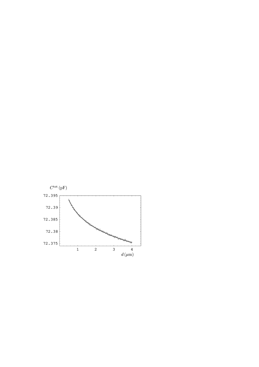
Figure 5: The measurement data for the total capacitance in a sphere-plane geometry for the experiment using a micromechanical torsional oscillator are indicated as gray dots. The solid line is the fit to the data using the model of a perfect spherical surface.

The results of capacitance measurements are shown in Fig. 5 as gray dots. These results were fitted to the total capacitance of the system given by the sum of the exact expression in Eq. (1) in a sphere-plate configuration, and the parasitic capacitance. The latter is given by $C^{\rm p}(a)=A^{\rm w}+A^{\rm pl}/z_{\rm meas}$ where $z_{\rm meas}$ is the separation between the end of the cleaved fiber and the platform. Here, the quantity $A^{\rm w}$ is separation independent, and is dominated by the capacitance between wires. The term $A^{\rm pl}/z_{\rm meas}$ models the capacitance of the plane capacitor formed by the cleaved fiber and the platform. We use the expression $z_{\rm meas}=d+D+b\theta$, where $\theta$ is negligibly small angle of rotation of the plate, $b$ is the lever arm, $d<D$, and $D$ does not depend on separation 15 ; 17 . The capacitance of the plane capacitor can then be represented as $A_{1}^{\rm pl}-A_{2}^{\rm pl}d/D$. Introducing the notations $\tilde{A}_{1}=A^{\rm w}+A_{1}^{\rm pl}$ and $\tilde{A}_{2}=A_{2}^{\rm pl}/D$, we can write the parasitic capacitance in the form

$$C^{\rm p}(d)=\tilde{A}_{1}-\tilde{A}_{2}d.$$ (18)

The fit of the results of capacitance measurements to the total theoretical capacitance $C^{\rm tot}(d)$, which is equal to the sum of expressions (1) and (18), was performed by the minimization of the function (17) with two unknown parameters $\tilde{A}_{1}$ and $\tilde{A}_{2}$. The resulting values of these parameters providing a minimum value to the quantity (17) are $\tilde{A}_{1}=72.32971\pm 0.00002\,$pF and $\tilde{A}_{2}=(2.18\pm 0.10)\times 10^{-4}\,\mbox{pF/$\mu$m}$. The plot of theoretical $C^{\rm tot}(d)$ versus separation is shown in Fig. 5 by the solid line. Taking into account that $n=351$ and the fit has $r=2$ parameters, we obtain for the number of degrees of freedom $f=349$. The resulting reduced $\chi^{2}$ is equal to 0.7 which leads to a probability to obtain not a smaller value of $\chi^{2}$ very close to unity. We emphasize that the fit was performed with respect to only two parameters of the parasitic capacitance which is determined by uncontrolled random factors. Thus, the obtaining of not a smaller value of $\chi^{2}$ in each next repetition of the measurement is really highly probable. The excellent agreement of our capacitance data with the model of a perfect spherical surface is seen in Fig. 5 where most of deviations of the data dots from the theoretical curve are in the limits of experimental errors. The seemingly larger scatter of the experimental dots around the solid line in Fig. 5, in comparison with Figs. 2 and 3(b), is explained by the different ranges of the variation of capacitance. In Figs. 2 and 3(b) capacitance varies by about 10 pF over the separation region of a few micrometers, but in Fig. 5 the variation of capacitance over the similar separation region is only 0.02 pF.

In the above fit we have used the exact expression in Eq. (1) for the capacitance in the configuration of a sphere above a plane. To discuss the usefulness of capacitance measurements, it is interesting to compare our results with those obtained when some approximate expression is used in the fit. For example, if we use the PFA, the capacitance is given by the leading, logarithmic, contribution on the right-hand side of Eq. (4) and the respective electric force by the first term (with $k=-1$) on the right-hand side of Eq. (5). The parasitic capacitance is represented by Eq. (18) as before. When we now perform the fitting procedure of the same data but using the simplified function

$$C^{\rm PFA}(d)=2\pi\epsilon_{0}R\ln\frac{R}{d}+\tilde{A}_{1}-\tilde{A}_{2}d,$$ (19)

the resulting values of the coefficients are $\tilde{A}_{1}=72.34530\pm 0.00002\,$pF and $\tilde{A}_{2}=(1.11\pm 0.10)\times 10^{-4}\,\mbox{pF/$\mu$m}$. They are slightly different from the case when the exact expression for the capacitance in the sphere-plane configuration has been used. What is important, however, is that the reduced $\chi^{2}$ for Eq. (19) is equal to 0.7, i.e., is the same as in the case of the exact Eq. (1). This means that it may be not possible to uniquely choose a preferable model when fitting several theoretical expressions to the experimental data of capacitance measurements with fitting parameters owing to the parasitic capacitances.

This does not mean, however, that the more exact and the less exact approximate analytical expressions for the capacitance and the electric force are equally applicable in electrostatic calibrations. For comparison purposes, in Table I we present the computational results for the capacitances (column 2–4) and the electric forces normalized by the factor $-(V-V_{0})^{2}$ (columns 5–7) at different separations (column 1). The values of the capacitances and electric forces are calculated using the exact expression in Eqs. (1) and (3) (columns 2 and 5, respectively), by the PFA, i.e., by the first terms in Eqs. (4) and (5) (columns 3 and 6), and using the more precise expansions in the powers of $d/R$ in Eqs. (8) and (5) (columns 4 and 7). As is seen in Table I (columns 2 and 3), for the capacitance, the PFA reproduces the exact results with a rather large relative error. When the separation varies from 0.5 to $4\,\mu$m, this error increases from 24.5% to 34.4%. Such large errors are explained by the fact that the PFA does not take into account the constant term in the capacitance [see Eq. (4)]. When such a constant $\tilde{A}_{1}$ is added to model the parasitic capacitances [see Eq. (19)], and is determined from the fit, it compensates for the missing separation-independent contribution in the theoretical expression provided by the PFA. As to the perturbative expansion for the capacitance in column 4, it is in much better agreement with the exact results in column 2. The respective relative error increases from 0.17% to only 1.86% when the separation increases from 0.5 to $4\,\mu$m.

With respect to the electric force measurements, the PFA (column 6) is in much better agreement with the exact results presented in column 5. Thus, with the increase of $d$ from 0.5 to $4\,\mu$m, the relative errors of the force values computed using PFA increase from 0.8% to only 4.7%. Such a good agreement is explained by the fact that the constant contribution to the capacitance, omitted in the PFA, does not influence the electric force. Even better agreement is found in Table I when comparing the force values computed using the perturbative expansion (column 7) with the exact values (column 5). Here, the relative error varies from 0.06% to 0.001% when the separation increases from 0.5 to $4\,\mu$m. Once again, it can be seen that the perturbative expansion for the electric force is much more exact than for the capacitance. This permits us to state that the primary role in the electrostatic calibrations of Casimir setups should be given to the electric force.

V Conclusions and discussion

In the foregoing we have considered the capacitance measurements as a part of the electrostatic calibrations in experiments on measuring the Casimir force. This subject was stimulated by Ref. 8 which reported the anomalous scaling law for the electric force in the configuration of a large lens above a plane plate, and the subsequent discussion 9 ; 10 ; 11 ; 12 . Keeping in mind the importance of electrostatic calibrations for the determination of the precision of the experimental results used in numerous applications of the Casimir force, a conclusive explanation of the puzzle is highly desirable. An attempt at such an explanation was undertaken in Ref. 10 by suggesting the model of a modified lens surface which reproduces the anomalous scaling law for the force observed in 8 . This explanation was disputed in Refs. 11 ; 12 by claiming that the suggested model is in much worse agreement with the results of capacitance measurements than the model of perfect spherical lens surface. Here, we demonstrate that the objections of Refs. 11 ; 12 against the model proposed in 10 are incorrect. As shown in Sec. III, instead of comparing the exact expression for the capacitance found in Ref. 10 with the corresponding experimental data, Ref. 11 made the comparison of the data with another function which does not reproduce the behavior of the exact expression of Ref. 10 . We have shown that the exact capacitance of Ref. 10 is in better agreement with the data than the one for an ideal spherical surface as used in Refs. 11 ; 12 . At the same time, we have also shown that the agreement with the data of both models of a lens surface modified near the closest point to the plate and of an ideal spherical surface is not satisfactory. This can be explained by the role of more irregularities distributed over a larger area of the surface of a centimeter size sphere which inevitably contribute to the capacitance.

To add important new information to this discussion, in Sec. IV we have presented new experimental data on the capacitance measurements in the Casimir setup using a micromechanical torsional oscillator 4 ; 15 ; 17 . This setup includes a perfectly shaped sapphire sphere of a radius 200 times smaller than the lens radius in Refs. 8 ; 11 ; 12 . The experimental data were carefully compared with the exact expression for the capacitance in a sphere-plane configuration. Different approximate representations for it, as discussed in Sec. II, were also analyzed. It was shown that the experimental data for the capacitance measurement in the setup using a micromechanical torsional oscillator are in excellent agreement with the model of a perfect spherical surface. This provides additional confirmation for the high quality of the Au-coated sapphire sphere used in that experiment.

One additional conclusion obtained in Sec. IV is that by using the capacitance measurements and by fitting them to different theoretical expressions it may be difficult to conclude which expression is in better agreement with data. The reason is that the capacitance measurements unavoidably contain a contribution from the parasitic capacitances which cannot be calculated theoretically with sufficient accuracy and whose parameters are determined from the fit. This permits us to conclude that the capacitance measurements in the electrostatic calibrations of the Casimir setups should be considered as an auxiliary tool providing an opportunity to confirm the good quality of the spherical surface used, and the correctness in the determination of absolute separations. In so doing the fitting of the data of the electric force measurements to the exact theoretical expression remains the main tool of electrostatic calibration in experiments on measuring the Casimir force.

                                                            

Figure 1: The capacitance (11) of a spherical lens with a modified geometry above a plane (the solid line) and its approximate expressions in Eq. (13) at large and in Eq. (12) at small separations (the dashed and dotted lines, respectively) versus separation.

                                                            

Figure 2: The measurement data for the capacitance in the lens-plane geometry versus voltage applied to the piezo are indicated as dots. The solid line is the fit to the data using the model of the modified geometry of the lens surface.

                                                            

Figure 3: Data for the capacitance measurements in the lens-plane geometry versus voltage applied to the piezo are indicated as dots. (a) Lines 1 and 2 and (b) the solid line are the fits to the data using the model of an ideal spherical surface with various parameters (see text for further discussion).

                                                            

Figure 4: The measurement errors of the capacitance in Ref. 11 versus voltage applied to the piezo are indicated as dots.

                                                            

Table 1: The values of the capacitances and electric forces [normalized on the factor $-(V-V_{0})^{2}$] in the sphere-plane geometry ($R=151.3\,\mu$m) computed by using the exact formulas (columns 2 and 5), the PFA (columns 3 and 6), and by the perturbative expansions (columns 4 and 7) at different separations (column 1).

	$C\,$(pF)			$-F/(V-V_{0})^{2}\,$(pF/m)
$d\,(\mu\mbox{m})$	exact	PFA	expansion	exact	PFA	expansion
0.5	0.06371	0.04808	0.06360	8350.23	8417.21	8355.18
1.0	0.05794	0.04225	0.05770	4148.06	4208.60	4149.75
1.5	0.05458	0.03884	0.05423	2748.97	2805.74	2749.56
2.0	0.05222	0.03641	0.05176	2050.22	2104.30	2050.40
2.5	0.05039	0.03454	0.04983	1631.44	1683.44	1631.47
3.0	0.04891	0.03300	0.04824	1352.56	1402.87	1352.56
3.5	0.04766	0.03170	0.04689	1153.59	1202.46	1153.58
4.0	0.04659	0.03058	0.04572	1004.54	1052.15	1004.53

References

- (1) H. B. G. Casimir, Proc. K. Ned. Akad. Wet. 51, 793 (1948).
- (2) G. L. Klimchitskaya, U. Mohideen, and V. M. Mostepanenko, ArXiv:0902.4022, Rev. Mod. Phys., to appear.
- (3) M. Bordag, G. L. Klimchitskaya, U. Mohideen, and V. M. Mostepanenko, Advances in the Casimir Effect (Oxford University Press, Oxford, 2009).
- (4) P. H. G. M. van Blockland and J. T. G. Overbeek, J. Chem Soc. Far. Trans. 74, 2637 (1978).
- (5) B. W. Harris, F. Chen, and U. Mohideen, Phys. Rev. A 62, 052109 (2000).
- (6) R. S. Decca, D. López, E. Fischbach, G. L. Klimchitskaya, D. E. Krause, and V. M. Mostepanenko, Ann. Phys. (N.Y.) 318, 37 (2005).
- (7) W. R. Smythe, Electrostatics and Electrodynamics (McGraw-Hill, New York, 1950).
- (8) F. Chen, U. Mohideen, G. L. Klimchitskaya, and V. M. Mostepanenko, Phys. Rev. A 74, 022103 (2006).
- (9) J. Blocki, J. Randrup, W. J. Swiatecki, and C. F. Tsang, Ann. Phys. (N.Y.) 105, 427 (1997).
- (10) W. J. Kim, M. Brown-Hayes, D. A. R. Dalvit, J. H. Brownell, and R. Onofrio, Phys. Rev. A 78, 020101(R) (2008).
- (11) S. de Man, K. Heeck, and D. Iannuzzi, Phys. Rev. A 79, 024102 (2009).
- (12) R. S. Decca, E. Fischbach, G. L. Klimchitskaya, D. E. Krause, D. López, U. Mohideen, and V. M. Mostepanenko, Phys. Rev. A 79, 026101 (2009).
- (13) W. J. Kim, M. Brown-Hayes, D. A. R. Dalvit, J. H. Brownell, and R. Onofrio, Phys. Rev. A 79, 026102 (2009).
- (14) W. J. Kim, M. Brown-Hayes, D. A. R. Dalvit, J. H. Brownell, and R. Onofrio, J. Phys.: Conf. Ser. 161, 012004 (2009).
- (15) E. Durand, Electrostatique, vol.2 (Masson, Paris, 1966).
- (16) L. Boyer, F. Houzé, A. Tonck, J.-L. Loubet, and J.-M. Georges, J. Phys. D: Appl. Phys. 27, 1504 (1994).
- (17) R. S. Decca, D. López, E. Fischbach, G. L. Klimchitskaya, D. E. Krause, and V. M. Mostepanenko, Phys. Rev. D 75, 077101 (2007); Eur. Phys. J. C 51, 963 (2007).
- (18) S. Brandt, Statistical and Computational Methods in Data Analysis (North-Holland, Amsterdam, 1976).
- (19) R. S. Decca and D. López, Int. J. Mod. Phys. A 24, 1748 (2009).