Quadrupolar correlations and spin freezing in $S=1$ triangular lattice antiferromagnets

Abstract

Motivated by experiments on NiGa₂S₄, we discuss characteristic (finite temperature) properties of spin $S=1$ quantum antiferromagnets on the triangular lattice. Several recent theoretical studies have suggested the possibility of quadrupolar (spin-nematic) ground states in the presence of sufficient biquadratic exchange. We argue that quadrupolar correlations are substantially more robust than the spin-nematic ground state, and give rise to a two peak structure of the specific heat. We characterize this behavior by a novel $T>0$ semiclassical approximation, which is amenable to efficient Monte Carlo simulations. Turning to low temperatures, we consider the effects of weak disorder on incommensurate magnetic order, which is present when interactions beyond nearest neighbor exchange are substantial. We show that non-magnetic impurities act as random fields on a component of the order parameter, leading to the disruption of long-range magnetic order even when the defects are arbitrarily weak. Instead, a gradual freezing phenomena is expected on lowering the temperature, with no sharp transition but a rapid slowing of dynamics and the development of substantial spin-glass-like correlations. We discuss these observations in relation to measurements of NiGa₂S₄.

I Introduction

The triangular lattice antiferromagnet has long been of interest because of its potential to exhibit exotic phases as a result of frustration and because it is the underlying lattice of many real materials. Unfortunately though, the simplest triangular lattice models have a well known tendency to order into states that are basically classical. For instance, it is generally believed that the nearest-neighbor spin 1/2 triangular lattice antiferromagnet orders into the 120-degree spiral state at zero temperature. However, since the models that describe real triangular lattice systems generally contain additional interactions, the possibilities for more interesting behavior remain vast.

One triangular lattice system that was recently proposed as a candidate for exotic behavior was the spin one antiferromagnet NiGa₂S₄, which exhibits no long-range spin ordering at zero temperature despite a low temperature susceptibility and specific heatNakatsuji et al. (2005) that suggest two-dimensional magnons; in particular, the specific heat grows very clearly as $T^{2}$ below $10K$. The specific heat furthermore shows no signs of a phase transition but instead shows two rounded peaks at $10K$ and $80K$, the latter being the Curie-Weiss temperature scale. Neutron scattering reveals the presence of short range magnetic ordering below $50K$ with an incommensurate wavevector; however, the magnetic correlation length never grows past about 7 lattice spacings even as the system is cooled to $1.5K$.Nakatsuji et al. (2005, 2007) More recent studies have shown that local moments do form and gradually freeze at low temperatures, fluctuating increasingly slowly as the temperature is reduced below $10K$.Takeya et al. (2008); Yaouanc et al. (2008); Maclaughlin et al. (2007) They eventually become static on the scale of the slowest available experimental local probe (muon spin resonance) below about $2K$.

A series of theoretical studies of this system subsequently appeared which attributed the thermodynamic signatures of ordering to a quadrupolar (also called spin-nematic) ground state stabilized by a nearest-neighbor biquadratic coupling term in the Hamiltonian. Tsunetsugu and Arikawa (2006); Läuchli et al. (2006); Bhattacharjee et al. (2006) Though such a state can account for the observed low temperature thermodynamics without requiring there to be any long-range spin ordering, it is inconsistent with the observed short-range incommensurate spiral order at the lowest temperatures. Moreover, the observation of static (though spatially random) spins at low temperatures casts doubt on the relevance of the spin-nematic phase to NiGa₂S₄. Indeed, to date no clear specific signature of even quadrupolar correlations (much less order) has been identified in NiGa₂S₄.

In this paper, we reconsider the principal experimental observations, and argue that such correlations are likely present in NiGa₂S₄, and signified by the unusual two peak structure in the specific heat. More formally, the double peak is a signature of proximity to a zero temperature quantum critical point between an antiferromagnetically ordered and a spin-nematic state. We also suggest a mechanism for the low temperature spin freezing, which is independent of the spin-nematic correlations. This mechanism should apply to any strongly two-dimensional magnet whose ground state in the absence of disorder is an incommensurate spiral. We argue that both these phenomena (the two peak specific heat and spin freezing) can be understood on purely symmetry grounds. Thus they may be expected to occur much more generally in other materials under conditions that we discuss.

For concreteness, we work within an extended model that not only includes the nearest-neighbor Heisenberg and biquadratic couplings, but also third-nearest-neighbor Heisenberg interactions:

$$H=J_{3}\sum_{[ij]}{\bf S}_{i}\cdot{\bf S}_{j}+J_{1}\sum_{\langle ij\rangle}{\bf S}_{i}\cdot{\bf S}_{j}-K\sum_{\langle ij\rangle}\left({\bf S}_{i}\cdot{\bf S}_{j}\right)^{2}.$$ (1)

The third neighbor couplings are denoted by $[ij]$ (on the triangular lattice, the third neighbor bonds point along the first neighbor bonds but doubled in length). This additional $J_{3}$ term is perhaps the simplest way to account for the observed order, which is described by a wavevector that is slightly less than half of the 120-degree state wavevector. Indeed, such an incommensurate spiral state is the exact solution of the classical limit of the above model in the limit $J_{3}>-J_{1}>K\geq 0$. Furthermore, detailed microscopic studies of NiGa₂S₄ indicate that a strong third-neighbor interaction is in fact present while second-neighbor interactions appear to be much less important. Mazin (2007); Takubo et al. (2007)

Let us outline our approach to the problem, and the layout of the remainder of the paper. For $J_{3}=0$, Eq. (1) has been analyzed already in Refs. Tsunetsugu and Arikawa, 2006; Läuchli et al., 2006, and shown to exhibit a non-magnetic but (ferro-)quadrupolar (spin-nematic) ground state in a broad parameter range. We argue that this remains true for the more general model with $J_{3}\neq 0$ in Sec. V. In addition, when $K$ is not too large, Eq. (1) has magnetically ordered ground states. Each of these states is connected to the quadrupolar one by a quantum phase transition (QPT). A major portion of this paper is concerned with establishing the $T>0$ properties of systems in the vicinity of such a QPT. We first present general symmetry-based arguments for the existence of two energy scales, and a resulting two peak structure of the specific heat, in Sec. II. To verify these ideas, we then introduce a novel “semiclassical SU(3)” or “sSU(3)” approximation, in which we can obtain these properties for Eq. (1) by classical Monte Carlo simulations. Though this approach is not expected to be quantitatively accurate for the $S=1$ model of interest, it does preserve all the symmetries of Eq. (1) and a qualitatively appropriate $T=0$ limit, unlike conventional semiclassical approaches. We carried out extensive numerical simulations using the sSU(3) approach to establish the nature of the $T>0$ phase transitions and crossovers, which we describe in Secs. IV and V.

Next, we turn to the effects of disorder, assuming that the putative ground state in the absence of impurities is magnetically ordered (though it may be near the QPT separating it from the quadrupolar phase). We show that the generic incommensurate spiral ground state of Eq. (1) is highly susceptible to defects. This is a direct consequence of the nature of the associated order parameter, which leads to strong “random field” effects of impurities – effects which do not pertain to the more conventional 120^∘ three-sublattice ground state. Moreover, very general arguments due to Imry and Ma show that such random field systems in two dimensions – but not in three – are always disordered. Hence we are led to conclude that the nature of the order parameter (which in turn is due to the large $J_{3}$ interaction) and the very weak three-dimensional coupling in NiGa₂S₄ are responsible for the observed low temperature glassy state. This mechanism for spin freezing is discussed in Sec. VI.2. We conclude the paper with a discussion in Sec. VII. The Appendix describes details of the measurements used in the Monte Carlo simulations.

II Symmetry and order parameters

In this section, we discuss the symmetries and order parameters of the Hamiltonian in Eq. (1) and its various proposed ground states. The Hamiltonian itself has global SU(2) spin-rotation symmetry, and the full space group symmetry of the triangular lattice. It is also time reversal invariant. A subset of these symmetries are retained in the various ground states. First, we discuss the conventional magnetically ordered states. We consider only coplanar spirals, which dominate the classical ground states of Eq. (1). In these states, the pattern of spin ordering is described by

$$\langle{\bf S}_{i}\rangle={\rm Re}\,\left[{\bf d}e^{i{\bf k}\cdot{\bf r}_{i}}\right],$$ (2)

where ${\bf d}=|d|({\bf\hat{e}}_{1}+i{\bf\hat{e}}_{2})$, with ${\bf\hat{e}}_{1},{\bf\hat{e}}_{2}$ orthogonal unit vectors, and ${\bf k}$ is the spiral wavevector. The spins lie in the plane spanned by ${\bf\hat{e}}_{1},{\bf\hat{e}}_{2}$, normal to ${\bf\hat{e}}_{3}={\bf\hat{e}}_{1}\times{\bf\hat{e}}_{2}$. Clearly, the spin spiral breaks spin rotational symmetry, and, assuming ${\bf k}\neq 0$, it does so completely: rotation by any angle about any spin axis alters the spin state. Moreover, under the same assumption, the spiral breaks translational symmetry. However, an important symmetry is retained by the coplanar spiral. In particular, under the combined action of a translation by any (lattice) vector ${\bf a}$, and a spin rotation by the angle ${\bf k}\cdot{\bf a}$ about the ${\bf\hat{e}}_{3}$ spin axis, the state is unchanged. The situation for spatial rotations is more complex. Consider the three-fold ($C_{3}$) rotation about a lattice site, a symmetry of the triangular lattice. In the familiar $120^{\circ}$ state (the ground state for $K=J_{3}=0$), the ordered spins remain invariant under this rotation, since the sublattices are unchanged. This invariance is, however, not generic. Formally, it can be traced to the fact that in this case, ${\bf k}$ is a zone-corner wavevector (the “K point”), which is invariant under such a rotation. Any other ${\bf k}$ is not invariant under a three-fold rotation, and moreover, the invariance cannot be regained by combining the spatial rotation with an SU(2) one. The breaking of the discrete $C_{3}$ rotation symmetry of $H$ implies that there are then three distinct “domains” of spiral state, with each of the three possible wavevectors forming an invariant set under the rotations. Each domain cannot be continuously transformed into another. This is quite different from the $120^{\circ}$ state, in which all possible spin configurations can be smoothly transformed into one another.

Next consider the (ferro)quadrupolar ground states. In them the ordered spin moment is zero:

$$\langle{\bf S}_{i}\rangle_{Q}=0.$$ (3)

However, the average magnetic quadrupole moment is non-zero:

$$Q_{i;\mu\nu} = \frac{1}{2}\langle\left\{S_{i}^{\mu},S_{i}^{\nu}\right\}\rangle-\frac{2}{3}\delta_{\mu\nu},$$ (4)

$$Q_{\mu\nu} = \frac{1}{N}\sum_{i}Q_{i;\mu\nu},$$ (5)

where $Q_{\mu\nu}$ is the (ferro-)quadrupolar order parameter. By construction, $Q$ is a traceless symmetric matrix. In the “spin-nematic” states which we consider, the eigenvalues of this matrix come in only two values, i.e. ${\rm eigs}(Q)=\{q,-q/2,-q/2\}$. More complicated “biaxial spin-nematic” states are possible in principle, in which all three eigenvalues are distinct. We will not consider them here, as there is no obvious reason for them to occur in Eq. (1). In the remainder of the paper, when we refer to the quadrupolar state, it will always be assumed to be of the (single axis) spin-nematic type. Then a general $Q$ can be written as

$$Q_{\mu\nu}=\frac{3}{2}q\left(\hat{n}_{\mu}\hat{n}_{\nu}-\frac{1}{3}\delta_{\mu\nu}\right),$$ (6)

where ${\bf\hat{n}}$ is a unit vector known as the “director”. The change of the director by a sign, ${\bf\hat{n}}\rightarrow-{\bf\hat{n}}$, has no physical significance, because $Q$ is even in ${\bf\hat{n}}$. The quadrupolar state breaks spin rotation symmetry, but retains invariance under spin rotations about the axis of the director. Furthermore, it retains full space group and time reversal symmetry.

Comparison of the symmetries of the magnetically ordered and quadrupolar ground states reveals an important fact: the symmetry group of the spiral state is a subgroup of the symmetry group of the quadrupolar one. Thus any order parameter of the quadrupolar state must already be non-zero in the magnetic phase. Indeed, within Landau theory, one expects a coupling between the magnetic and quadrupolar order parameters, i.e. a term in the free energy density $f$ of the form

$$f_{Q-d}=\lambda Q_{\mu\nu}\left[d_{\mu}^{*}d_{\nu}^{\vphantom{*}}+d_{\nu}^{*}d_{\mu}^{\vphantom{*}}-\tfrac{2}{3}{\bf d}^{*}\cdot{\bf d}^{\vphantom{*}}\delta_{\mu\nu}\right],$$ (7)

where $\lambda$ is a non-zero coupling constant. This generically induces a non-zero $Q_{\mu\nu}$ of the form in Eq. (6), with $|q|\propto|d|^{2}$ and ${\bf\hat{n}}={\bf\hat{e}}_{3}$.

It follows that $q$ in Eq. (6) remains non-zero across the QPT between the magnetic and quadrupolar states. Conversely, at this QPT, presuming it is continuous or weakly first order, the magnetic order parameter ${\bf d}$ becomes arbitrarily small. Associated with each of these order parameters is an energy scale, describing the energy needed to disturb the order parameter locally. This energy is supplied with increasing temperature, releasing entropy associated with the ordering. As usual, the specific heat is expected to show a peak at this characteristic temperature (whose precise nature requires more detailed considerations of symmetry, universality, and energetics). Near the QPT, on the magnetically ordered side, one is then led to expect two widely separated energy scales: the quadrupolar “ordering” scale, which remains of $O(1)$ (i.e. not parametrically small near the QPT), and a much smaller magnetic “ordering” scale, which vanishes on approaching the QPT. There will be a specific heat peak at each of these temperatures. The schematic phase diagram is shown in Fig. 1. We have used “ordering” in quotes, because in a two-dimensional system, the continuous order parameters are prohibited from exhibiting long-range order by the Mermin-Wagner theorem. However, the specific heat is dominated by short distance correlations, and exhibits peaks regardless of the presence or absence of true phase transitions.

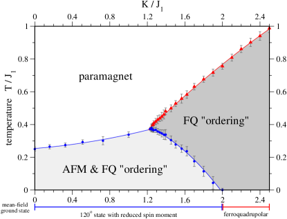
Figure 1: Finite temperature phase diagram of the nearest-neighbor only model with antiferromagnetic $J_{1}>0$ and a ferronematic $K>0$ obtained from numerical simulations in the sSU(3) approximation. The location of the phase boundaries are obtained from the position of the specific heat peaks in our numerical simulations. Approaching zero temperature the semiclassical sSU(3) approximation recovers the ground states obtained in mean-field theory. We note that the phase boundaries indicate a rapid growth of the ferroquadrupolar and magnetic correlation lengths, but not true long-range order excluded by the Mermin-Wagner theorem.

III Semiclassical SU(3) Approximation

In the previous section, we argued for the emergence of two temperature scales and a two peak structure in the specific heat, whenever the system is in vicinity of the QPT between an antiferromagnetic and quadrupolar ground state. In what follows, we will check these arguments by explicit calculations of $T>0$ properties. To do this presents a serious difficulty: theoretical approaches to calculate the low but nonzero temperature behavior of frustrated quantum Hamiltonians are extremely limited. A direct attack with quantum Monte Carlo is prevented by the sign problem, and many other approaches (e.g. variational wavefunctions, Lanczos diagonalization) are restricted to ground state properties.

One natural approach is the classical approximation, in which the quantum spin operators are replaced by continuous classical vectors of length $S$. For many quantum spin models, the success of spin-wave theory, even for low spin, proves the applicability of this method. However, for the study of Eq. (1), such an approach is fatally flawed. The difficulty lies in the highly quantum nature of the quadrupolar spin-nematic correlations induced by the biquadratic interaction for spin $S=1$. In particular, the ferronematic ground states favored by $K>0$ are of “easy-plane” type, in which the spins may be thought of as fluctuating quantum mechanically in the plane perpendicular to the director $\hat{n}$ in Eq. (6). This corresponds to the sign $q<0$. For large spin, including the classical limit, however, the biquadratic interaction with $K>0$ favors collinear states of the spins, and hence “easy axis” rather than easy-plane ferronematic order (with the opposite sign of $q$). In a simple mean-field theory, the nature of the quadrupolar order changes from easy plane when $S\leq 2$ to easy axis for $S>2$. Therefore even qualitatively the classical vector spin approximation fails to capture the proper ferronematic correlations of the physics $S=1$ system.

We thus follow an alternative approach, which generalizes the zero temperature variational approach of Ref. Läuchli et al., 2006 to $T>0$. In that work, a trial ground state was taken to be entanglement-free, i.e. of direct product form:

$$|\Psi\rangle=\otimes_{i}|\psi_{i}\rangle,$$ (8)

with an arbitary spin $S=1$ state $|\psi\rangle_{i}$ on site $i$. A general single spin state can be written as

$$|\psi_{i}\rangle=b_{i1}|x\rangle+b_{i2}|y\rangle+b_{i3}|z\rangle\ ,$$ (9)

with an arbitary complex vector ${\bf b}_{i}$ satisfying the normalization constraint that ${\bf b}^{*}_{i}\cdot{\bf b}_{i}=1$. Here we have used the time-reversal invariant basis of $S=1$ states defined by

$$|x\rangle = i\left(\frac{1}{\sqrt{2}}|1\rangle-\frac{1}{\sqrt{2}}|\bar{1}\rangle\right)$$

$$|y\rangle = \frac{1}{\sqrt{2}}|1\rangle+\frac{1}{\sqrt{2}}|\bar{1}\rangle$$

$$|z\rangle = -i|0\rangle$$

where $|1\rangle$,$|0\rangle$ and $|\bar{1}\rangle$ are the usual $S=1$ states quantized along the z-axis. These basis states are null vectors of their respective spin components, i.e. $S^{x}|x\rangle=S^{y}|y\rangle=S^{z}|z\rangle=0$. Semiclassically, the state $|x\rangle$ may be viewed as one in which the spin fluctuates primarily in the yz-plane (and similarly for the other two states).

The expectation values of the spin and quadrupolar operators have simple expressions in these states:

$$\langle\psi_{i}|{\bf S}_{i}|\psi_{i}\rangle = -i{\bf b}_{i}^{*}\times{\bf b}_{i}^{\vphantom{*}},$$ (10)

$$Q_{i;\mu\nu} = \frac{1}{3}\delta^{\mu\nu}-\frac{1}{2}\left(b_{i\mu}^{\dagger}b_{i\nu}^{\vphantom{\dagger}}+b_{i\nu}^{\dagger}b_{i\mu}^{\vphantom{\dagger}}\right).$$

Note that when ${\bf b}_{i}$ is real (it may be multiplied by an overall phase without affecting physical properties), the spin expectation vanishes. Thus in this case it may be interpreted as the nematic director, i.e. ${\bf b}_{i}={\bf\hat{n}}_{i}$. Adding an imaginary part to ${\bf b}_{i}$ produces a nonzero spin moment that is orthogonal to the plane in which the real and imaginary parts of ${\bf b}_{i}$ lie.

From Eq. (10), we can compute the expectation value of the Hamiltonian,

$$H_{\rm cl} \equiv \langle\Psi|H|\Psi\rangle$$

$$= J_{3}\sum_{[ij]}|{\bf b}^{*}_{i}\cdot{\bf b}_{j}|^{2}-|{\bf b}_{i}\cdot{\bf b}_{j}|^{2}$$

$$\mbox{}+\sum_{\langle ij\rangle}J_{1}|{\bf b}^{*}_{i}\cdot{\bf b}_{j}|^{2}-(J_{1}+K)|{\bf b}_{i}\cdot{\bf b}_{j}|^{2}\ .$$

In Ref. Läuchli et al., 2006, this expression was minimized for the nearest-neighbor model ($J_{3}=0$) to find variational ground states. It was found that the variational approximation qualitatively reproduced the correct $T=0$ phase diagram, though it incorrectly determined the quantitative location of the ferronematic-antiferromagnetic phase boundary. Note that, at $T=0$, the variational approximation is equivalent to a mean-field theory in which the expectation values $Q_{i;\mu\nu}$ and $\langle{\bf S}_{i}\rangle$ are self-consistently determined from a Hamiltonian of decoupled $S=1$ spins.

To address $T>0$ temperature properties, we follow an unusual procedure of elevating Eq. (III) to a Hamiltonian of a two-dimensional statistical mechanical model, allowing the classical ${\bf b}_{i}$ vectors to fluctuate thermally with the Boltzmann weight $\exp[-\beta H_{\rm cl}]$. Because in this new classical problem, the “spins” appear as three-component complex vectors, and transform under symmetries by rotations by unitary three-dimensional matrices, we call this treatment the semiclassical SU(3) or sSU(3) approximation, and the resulting statistical mechanical problem the sSU(3) model. We emphasize, however, that the model Eq. (III) does not have SU(3) symmetry, but only the physically appropriate SU(2) spin rotational and lattice symmetries.

The sSU(3) model can be understood as a leading-order term in a cumulant expansion of the full quantum partition function. Specifically, we approximate

$$Z = {\rm Tr}\,e^{-\beta H}$$

$$= \int\prod_{i}d\Omega_{b_{i}}\langle\Psi(b)|e^{-\beta H}|\Psi(b)\rangle$$

$$\approx \int\prod_{i}d\Omega_{b_{i}}e^{-\beta\langle\Psi(b)|H|\Psi(b)\rangle}=\int\prod_{i}d\Omega_{b_{i}}e^{-\beta H_{cl}},$$

where $d\Omega_{b}=(2\pi)^{2}[\prod_{\mu=x,y,z}d{\rm Re}\,b_{\mu}d{\rm Im}\,b_{\mu}]\delta(\sum_{\mu}|b_{\mu}|^{2}-1)$ is the appropriately normalized measure over unit 3-component complex vectors, such that $\int d\Omega_{b}1={\rm Tr}1=3$. From this perspective, we see that the sSU(3) approximation becomes exact at high temperatures (reproducing the exact free energy to $O(\beta)$ in the $\beta$ expansion), and approaches the variational result as $T\rightarrow 0$. It can therefore be expected to yield a reasonable qualitative approximation to the physics over the full range of intermediate temperatures.

One may consider at this stage, given that the $T=0$ variational approach is equivalent to mean-field theory, why not instead apply the usual mean-field theory at $T>0$? The reason to choose the sSU(3) approach is that it captures much better the effects of thermal fluctuations, which are very important in a two-dimensional system. For instance, because Eq. (III) has the physically correct symmetries, we expect by universality that it displays the correct exact critical behavior at any $T>0$ phase transitions. Moreover, it avoids spurious transitions which are in fact prohibited by the Mermin-Wagner theorem. In contrast, straight mean-field theory will produce sharp phase transitions associated with quadrupolar and magnetic ordering, neither of which are in fact allowed in two dimensions.

Despite the above advantages of the sSU(3) approximation over mean-field theory, it is very amenable to numerical computations. The classical Hamiltonian in Eq. (III) is completely real, so there is manifestly no sign problem. The only subtlety lies in the gauge redundancy of the ${\bf b}_{i}$ variables, whose phase (on each site) has no physical significance. However, no difficulty is incurred in Monte Carlo simulations by simply including the redundancy, and restricted measurements to gauge-invariant observables. For our numerical simulations of this semiclassical Hamiltonian we have built our implementation of a classical Monte Carlo algorithm on the ALPS libraries A.F. Albuquerque et al. (2007), and in particular expanded its classical Monte Carlo application code to sample configurations of the three-component complex vectors or “spins” as introduced above. We give a detailed account of how to measure various physical observables in this Monte Carlo scheme in the Appendix.

IV Finite Temperature Properties of the Nearest-Neighbor Model

As a first step we apply the semiclassical sSU(3) approximation to numerically analyze the $T>0$ thermodynamic features and correlations of the simplest, nearest-neighbor Hamiltonian with biquadratic exchange

$$H=J_{1}\sum_{\langle ij\rangle}{\bf S}_{i}\cdot{\bf S}_{j}-K\sum_{\langle ij\rangle}\left({\bf S}_{i}\cdot{\bf S}_{j}\right)^{2}\,,$$ (13)

where we consider antiferromagnetic $J_{1}>0$ and ferronematic $K>0$. Though our primary focus will be on finite temperature properties of this model, it is helpful to begin by reviewing what is already known about its ground states.

IV.1 Ground State Properties

The full zero temperature phase diagram of the nearest-neighbor bilinear-biquadratic model contains the conventional ferro- and antiferromagnetic magnetic phases when $K$ is small, but also includes a ferroquadrupolar phase and an antiferroquadrupolar phase stablized by larger values of $K$.

In the range of parameters of interest to us ($J_{1}$ and $K$ positive), there is a single quantum phase transition as shown in Fig. 1. For small $K/J_{1}$, the ground state is a 120-degree spiral ground state with a reduced spin moment. Then, as $K/J_{1}$ is increased, the spin moment decreases to zero leaving a state with only ferroquadrupolar order i.e. no average spin moment but an identical director (identical, real ${\bf b}$) on every site. In the mean-field/variational approximation, this phase transition happens precisely at $K/J_{1}=2$. Exact diagonalization results Läuchli et al. (2006) for the quantum model show, however, that quantum fluctuations strongly reduce this value to about $K/J_{1}=0.4$.

Within mean-field theory, a detailed study shows that the quadrupolar to antiferromagnetic quantum phase transitions is continuous. Thus this model fits nicely into the framework discussed in Sec. II: For any finite $K/J_{1}$ up to the critical value, the Néel and ferroquadrupolar orders actually coexist, leading to a smooth reduction in the value of $|\langle{\bf S}\rangle|$ as $K$ is increased.

IV.2 Separation of Temperature Scales

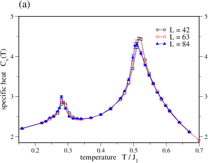
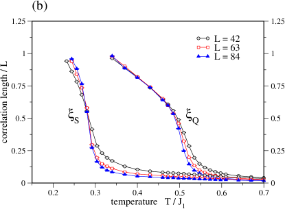
Figure 2: Finite temperature calculations of (a) the specific heat and (b) the spin and quadrupolar correlation lengths $\xi_{S}$ and $\xi_{Q}$ for the nearest-neighbor model in the semiclassical sSU(3) approximation. The two temperature scales associated with the rapid growth of magnetic and ferroquadrupolar correlations result in a characteristic two peak structure of the specific heat. The data shown is for couplings $K/J_{1}=1.5$ and system sizes chosen to be commensurate with the low-temperature spin ordering.

We have argued above that close to such a quantum phase transition from spiral to quadrupolar order a spin system may develop significant quadrupolar correlations at a distinct, higher temperature scale than the one associated with the rapid growth of magnetic correlations. Our numerical simulations of the sSU(3) model associated with Hamiltonian (13) does indeed reveal such a characteristic separation of temperature scales for $K/J_{1}$ sufficiently close to the quantum phase transition which in mean-field approximation occurs at $K/J_{1}=2$.

In particular, we find that in the proximity of the quantum phase transition $K/J_{1}<2$ the measured specific heat develops two distinct peaks as illustrated in Fig. 2. Calculating the ferroquadrupolar and magnetic correlation lengths, we can associate the upper peak with the rapid growths of ferroquadrupolar correlations while the lower peak indicates the onset of magnetic correlations (with a wavevector of length $4\pi/3$ that is characteristic of the 120-degree state). We note that although the correlation lengths grow to be very large below each of the two temperature scales, they remain finite, consistent with the absence of long-range order. While the high temperature peak in the specific heat shows no singular behavior as we cross the location of the quantum phase transition at $K/J_{1}=2$, we find that the lower peak approaches zero-temperature exactly at the QPT. For smaller values of $K/J_{1}<2$ the two peaks get closer and eventually merge around $K/J_{1}\approx 5/4$, below which we only observe one temperature scale indicated by a single peak in the specific heat.

We summarize our results for the nearest-neighbor model (13) in the phase diagram of Fig. 1, where the phase boundaries indicate the locations of the respective peaks in the calculated specific heat. Note that these phase boundaries are not phase transitions, due to the absence of long-range order as mandated by the Mermin-Wagner theorem.

Finally, we note that the numerical results of our sSU(3) approximation are not expected to be quantitatively correct, as it becomes clear from the quantitative discrepancy to exact diagonalization results. However, we emphasize that the key ingredient underlying our qualitative results is a continuous quantum phase transition in which the magnetic order smoothly vanishes but the quadrupolar order survives in both phases. As long as the full inclusion of quantum effects does not lead to the zero temperature phase transition actually becoming strongly first order, then a separation of temperature scales should generically be observed when the parameters of this system are near the quantum critical region.

V The $J_{3}$-$J_{1}$-$K$ Model

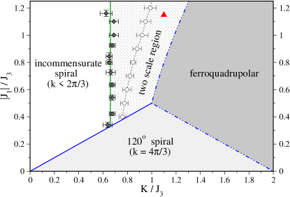
Figure 3: Zero temperature phase diagram of the model with antiferromagnetic third-nearest-neighbor coupling $J_{3}$ and nearest-neighbor ferromagnetic $J_{1}$ and ferronematic $K$ couplings obtained from numerical simulations in the sSU(3) approximation. The three phases present at zero temperature have a ferroquadrupolar, 120 degree spiral or incommensurate spiral ground state, with continuous transitions (dashed lines) between the ferroquadrupolar and spiral states and a first-order transition between the 120 degree and incommensurate spiral states. The cross-hatched area marks the region where our finite temperature calculations indicate two temperature scales. Such a separation is observed both in specific heat (filled diamonds) and correlation length measurements (open circles) which are expected to coincide in the thermodynamic limit. The red triangle marks the location of the representative system, for which we show finite temperature properties in Fig. 4.

We now turn to the full model in Eq. (1) including a third-nearest-neighbor coupling, which is necessary to properly capture incommensurate magnetic correlations at low temperatures. We assume antiferromagnetic third-neighbor interactions $J_{3}>0$ and ferronematic $K>0$ (as before), but now consider a ferromagnetic nearest-neighbor coupling $J_{1}<0$. It is this combination of couplings that will realize the proper magnetic correlations observed in NiGa₂S₄. As we shall see, the presence of an incommensurate spiral ground state has interesting consequences in that it introduces a true finite temperature phase transition associated with anisotropic spin fluctuations.

While we find that the above model can now account for the type of magnetic order observed in NiGa₂S₄, it still cannot explain the fact that the spin order never grows to be long ranged and exhibits slow dynamics. Therefore we will ultimately have to consider the role of disorder before discussing our results in the context of the real material.

V.1 Ground States

We again start our analysis of of Hamiltonian (1) by discussing its zero temperature phase diagram calculated in mean-field approximation. For the range of parameters of interest, we assume that it is sufficient to take the magnetic ground states to be coplanar and invariant under the combination of a lattice translation and spin rotation associated with a single wavevector. Under these two assumptions, the most general possible choice for the vector of amplitudes ${\bf b}_{i}$ describing the wavefunction at a single site is, up to a global O(3) spin rotation,

$${\bf b}_{i}=\left[\begin{array}[]{l}\sin\theta\cos({\bf k}\cdot{\bf r}_{i})e^{i\alpha}\\ \sin\theta\sin({\bf k}\cdot{\bf r}_{i})e^{i\alpha}\\ \cos\theta\end{array}\right]\,.$$

Minimizing the energy over the variables ${\bf k}$, $\theta$ and $\alpha$ we obtain the zero temperature phase diagram shown in Fig. 3. For small values of $K/J_{3}$, the ground states are again spirals with a reduced spin moment. Along the line $|J_{1}|=K/2$ for $K<1$, the wavenumber describing these spiral states ground states jumps from $4\pi/3$ to $2\pi/3$ and then continuously decreases to zero with increasing $|J_{1}|$, ultimately leading to a ferromagnetic ground state for very large values of $|J_{1}|/J_{3}$. The new feature in this phase diagram is thus a large region of parameters for which the spiral is incommensurate (with wavevector $k<2\pi/3$). Increasing the biquadratic exchange $K$ for fixed $|J_{1}|/J_{3}$, these spiral ground states smoothly transform into a ferroquadrupolar ground state with $\langle{\bf S}\rangle=0$ which is the ground state for large $K$.

V.2 Separation of Temperature Scales

Similar to the nearest-neighbor only model we expect on symmetry grounds that also the model with third-neighbor interactions exhibits a separation of temperature scales in the vicinity of the continuous quantum phase transition between the ferroquadrupolar and (incommensurate) spin spiral state. Indeed our numerical simulations of this model in the sSU(3) approximation reveal a broad range of couplings in the vicinity of this line of continuous transtions where both specific heat and correlation length measurements indicate two different temperature scales as indicated by the cross-hatched area in Fig. 3.

In agreement with the symmetry arguments in support of this temperature scale separation we again find that the upper temperature scale corresponds to the rapid growth of quadrupolar correlations while the lower temperature is associated with the onset of magnetic correlations. Numerical data for a representative choice of parameters (indicated by the red triangle in Fig. 3) is shown in Fig. 4, where we plot the specific heat and correlation length measurements as before. The exact parameters $K/J_{3}=1.1$ and $J_{1}/J_{3}\approx-1.14855$ and system sizes are again chosen such that the low temperature spiral state has a commensurate spatial period (in this case 7 lattice spacings) which in turn allows to compute the correlation lengths directly from the respective structure factors.

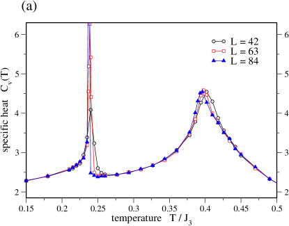
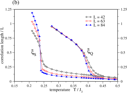
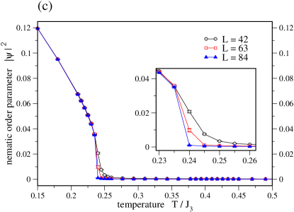
Figure 4: Finite temperature calculations of (a) the specific heat, (b) the spin and quadrupolar correlation lengths $\xi_{S}$ and $\xi_{Q}$ and (c) the nematic order parameter $|\psi|^{2}$ for the model with third-nearest-neghbor interaction in the semiclassical sSU(3) approximation. The two temperature scales associated with the rapid growth of magnetic and ferroquadrupolar correlations again result in a characteristic two peak structure of the specific heat. The data shown is for couplings $K/J_{3}=1.1$ and $J_{1}/J_{3}=-1.14855$ and system sizes chosen to be commensurate with the low-temperature spin ordering. In contrast to the nearest-neighbor model, we see a divergent lower peak corresponding to the breaking of lattice rotational symmetry by anisotropic spin fluctuations.

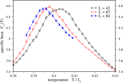
Figure 5: Finite-size scaling of the upper peak in the specific heat of the representative system with couplings $K/J_{3}=1.1$ and $J_{1}/J_{3}=-1.14855$. While the peak slightly shifts with increasing system size, there is clearly no divergence.

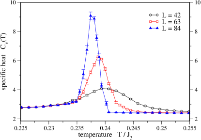
Figure 6: Finite-size scaling of the lower peak in the specific heat of the representative system with $K/J_{3}=1.1$ and $J_{1}/J_{3}\approx-1.14855$. The trend with increasing system size clearly suggests a divergence in the thermodynamic limit.

V.3 C₃ Bond Ordering Transition

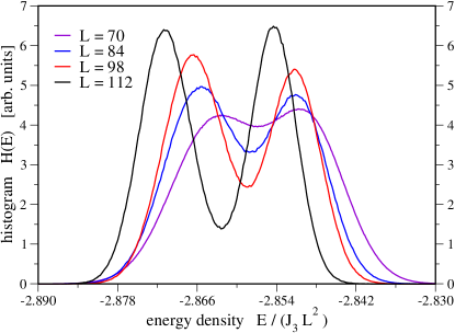
Figure 7: Histogram of the energy density for our representative system in the vicinity of the low temperature transition. The bimodal character of this distribution proliferates with increasing system size, which is indicative of a first-order transition. Data for different system sizes/temperatures are shown; in particular $L=84$ ($T/J_{3}=0.2377$), $L=98$ ($T/J_{3}=0.2374$), and $L=112$ ($T/J_{3}=0.2361$).

As ferroquadrupolar correlations only break the continuous SU(2) symmetry, the transition at the upper temperature scale should not be associated with the onset of true long-range order as mandated by the Mermin-Wagner theorem. Indeed a finite-size scaling analysis of our numerical data shows that the high-temperature peak in the specific heat is non-divergent as we increase the system size, as illustrated in Fig. 5.

A similar analysis for the transition at the lower temperature scale, however, reveals that more interesting things can happen. For any choice of parameters that puts the ground state of the system into the incommensurate spiral phase, the lower peak of the specific heat appears to diverge sharply as shown in Figs. 4(a) and 6. This divergence indicates a true phase transition, which in two dimensions must reflect the breaking of some discrete symmetry in accordance with the Mermin-Wagner theorem. (In principle such a divergence could also be explained by a first-order transition without a change of symmetry, but will be ruled out below.)

The key observation to explain this phase transition to a long range ordered state is that any (incommensurate) spiral state on the triangular lattice with wavenumber $|k|<4\pi/3$ exhibits spin correlations that are stronger along one axis than the other two, unlike the 120-degree state, in which every spin differs from its neighbors by the same angle. Therefore any incommensurate spiral state spontaneously breaks the discrete $C_{3}$ rotational symmetry of the lattice and there is nothing to prevent this symmetry breaking from occurring at a finite temperature. Indeed, it has recently been shown that the related classical model with O(3) spins on the triangular lattice and first and third neighbor exchange spontaneously breaks the $C_{3}$ lattice rotation symmetry at low temperature Tamura and Kawashima (2008). In the $C_{3}$ broken state the system exhibits “bond order” in the sense that the exchange energies for bonds along different principle axes become distinct.

To confirm that the lower temperature scale in our sSU(3) model does indeed correspond to the breaking of lattice rotational symmetry, we define a bond order parameter $\psi$, which is nonzero only in the presence of anisotropic spin correlations:

$$\psi=\frac{1}{N}\sum_{i,\mu}(a^{x}_{\mu}+ia^{y}_{\mu})\,\langle{\bf S}_{{\bf r}_{i}}\cdot{\bf S}_{{\bf r}_{i}+{\bf a}_{\mu}}\rangle\,,$$

where ${\bf a}_{1}=\hat{x}$ and ${\bf a}_{2,3}$ are its rotations by $2\pi/3$ and $4\pi/3$, respectively. This order parameter is a complex number whose argument reveals the direction of the strongest correlations and whose magnitude for a spiral state with wavenumber $k$ is given by

$$|\psi|=\langle|{\bf S}|\rangle^{2}\,[\cos(k)-\cos(k/2)]\ .$$

Moreover, we note that $\psi$ is invariant under the transformation ${\bf S}_{i}\rightarrow-{\bf S}_{i}$ and under a lattice rotation of angle $\pi$. Thus, any nonzero value of $\psi$ indicates that the system is one of three inequivalent bond ordered phases related to each other by lattice rotations of $2\pi/3$ (cf. the discussion on spiral magnetic domains in section II).

Measurements of this bond order parameter for the sSU(3) model associated with Hamiltonian (1) confirm that the system enters a bond ordered state for couplings leading to an incommensurate spiral ground state, as shown in Fig. 4 (c) for our representative system. To determine the order of this low temperature transition we have measured energy histograms in the vicinity of the transition temperature. The bimodal histogram distribution, shown in Fig. 7, unambiguously points to a first-order transition, which is also indicated by the narrow peak in the specific heat and the apparent jump of the magnetic correlation length in Fig. 4 (b). Thus the C₃ transition in the sSU(3) model has the same qualitative properties as the corresponding transition in the O(3) model which was also found to be first order Tamura and Kawashima (2008).

VI Disorder

VI.1 Imry-Ma argument and correlation lengths

We now turn to the effects of disorder. We consider sulfur (S) vacancies to likely be the dominant type of impurity in NiGa₂S₄. However, our analysis will be rather general, and rely only upon the assumption that the defects are uncorrelated, local, and non-magnetic. On symmetry grounds, non-magnetic disorder couples directly to the $C_{3}$ order parameter, but not to ${\bf d}$, since (neglecting spin-orbit) it respects SU(2) symmetry. Thus for the $C_{3}$ order, the impurities act as “random fields”. In two dimensions, the standard Imry-Ma argument implies that long-range $C_{3}$ order is destroyed by arbitrarily weak disorder.Nattermann (1997) The system breaks up into “domains”, leading to a saturation of the correlation length $\xi_{C_{3}}$ for the $C_{3}$ bond order. We parametrize the strength of the random field by an energy $\Delta$, which gives e.g. the range of variation in strength of exchange couplings due to S vacancies. The essence of the Imry-Ma argument is a competition between the surface energy required to nucleate a domain of one phase within another, and the energy gain that can be obtained from the random fields within the domain. The former is proportional to the surface tension $\sigma$ of a domain, while the latter is proportional to $\Delta|\psi|$. Hence we expect $\xi_{C_{3}}$ to be a function of $\sigma/(\Delta|\psi|)$. According to the Imry-Ma argument,Nattermann (1997) two dimensions is the marginal (lower critical) dimension for the stability of the ordered state. Hence the correlation length is an exponential function of the disorder strength. We arrive at the conclusion

$$\xi_{C_{3}}(T)\sim\exp\left[\frac{c\sigma(T)^{2}}{\Delta^{2}|\psi(T)|^{2}}\right],$$ (14)

with some constant $c$. At $T\ll T_{C_{3}}$, we expect $\sigma(0)\sim O(J_{3})$ and $\psi(0)\sim O(1)$. Eq. (14) describes a continuous decrease of the $C_{3}$ correlation length on increasing temperature up to $T\approx T_{C_{3}}$, the temperature of the $C_{3}$ transition of the pure system. At this point, the first order transition of the pure system will be rounded by disorder, and the $C_{3}$ correlation length will smoothly (and quickly) approach its finite value for the pure system for $T>T_{C_{3}}$.

What of the magnetism? Although the magnetic order parameter does not couple direction to disorder, it will be strongly affected by the domain structure. In particular, the conventional spiral correlation length will saturate at the domain size,

$$\xi_{M}(\Delta,T)\approx\min\,\left[\xi_{M}(0,T),\xi_{C_{3}}(\Delta,T)\right].$$ (15)

Because the pure system’s magnetic correlation length grows very large below $T_{C_{3}}$, we expect that for most if not all of this temperature range, that simply $\xi_{M}=\xi_{C_{3}}\equiv\xi$.

VI.2 Correlations on longer scales: gauge glass physics

The finiteness of the above correlation lengths does not imply a complete absence of magnetic correlations beyond this length scale, only that the spiral correlations remain short range. One longer scales, we need to consider more subtle correlations between spins in different domains.

In what follows, we will make a simplifying assumption, that the spirals are fixed in the XY plane. This could be justified by a small easy-plane anisotropy, $H_{\rm anis}=D\sum_{i}\left(S_{i}^{z}\right)^{2}$, which is expected to be present, but small, in NiGa₂S₄. Provided $D\xi^{2}\gtrsim k_{B}T$, which will be satisfied at low enough temperatures, the spins will indeed lie in the XY plane. It may also be the case that the spins adopt a coplanar state spontaneously, even in the absence of magnetic anisotropy. However, we do not make a definitive statement in this respect. Should this assumption fail, we expect that this approximation underestimates the fluctuations, and therefore overestimates the tendency to spin freezing. One should probably therefore view the estimates of the spin glass correlation length and time below as upper bounds.

To proceed, we define ${\bf d}_{i}=({\bf\hat{x}}+i{\bf\hat{y}})e^{i\theta_{i}}$ as the average order parameter for a domain $i$, within which the wavevector is fixed at ${\bf Q}_{b_{i}}$. In general, the energy of the system will depend upon the difference of the angles $\theta_{i}-\theta_{j}$ in adjacent domains, due to the coupling of spins at the domain boundaries. This coupling is complicated and depends upon the specific structure of this boundary, and the wavevectors of the two domains. Therefore we will assume the effective Hamiltonian

$$H_{\rm eff}=-K\sum_{\langle ij\rangle}\cos(\theta_{i}-\theta_{j}-\alpha_{ij}),$$ (16)

where $\alpha_{ij}$ is a random variable, which we take to be independent on each $ij$ and uniformly distributed between $0$ and $2\pi$. We have neglected for simplicity randomness in the magnitude of the coupling between domains, which does not qualitatively affect the physics. The coefficient $K$ arises from adding the exchange couplings along the boundary of the two domains in question. If the addition is constructive, we expect, ignoring fluctuations $K\sim J_{3}\xi$, or if it is random instead $K\sim J_{3}\sqrt{\xi}$. With thermal and/or quantum fluctuations, this should be reduced by a factor of $\langle|d|^{2}\rangle$. Assuming a mean-field temperature dependence of the magnitude of the local spiral order parameter, one finds a smooth reduction with increasing temperature $K(T)=K(0)(1-T/T_{MF})$, for $T<T_{MF}$. Generally, $K\gg k_{B}T$ in the regime where we can apply Eq. (16).

Eq. (16) is the Hamiltonian of the two-dimensional gauge glass model, which has been intensively studied in the past.Fisher and Huse (1988); Katzgraber and Young (2002); Nikolaou and Wallin (2004); Fisher et al. (1991) It is believed that its lower critical dimension is greater than two, so that the system is disordered (paramagnetic) at all $T>0$.Nikolaou and Wallin (2004) However, the correlation length for glassy (Edwards-Anderson) order, and the correlation times of the spins, diverge rapidly as $T\rightarrow 0$.

To understand this behavior in more detail, we must discuss the excitations of the gauge glass ground state. Obviously, because of the global $U(1)$ symmetry of Eq. (16), there are Goldstone-type spin waves, in which the phases $\theta_{i}$ vary slowly away from their ground state values. These are the Halperin-Saslow modes, introduced in Ref. Halperin and Saslow, 1977 and discussed in Ref. Podolsky and Kim, 2009 in the context of NiGa₂S₄. More subtle, however, are non-smooth deformations of the phase, which have lower energy than the spin waves for a corresponding length scale. These are the “droplets” of the droplet theory.Fisher and Huse (1988) From numerical studies, these have a classical energy $E\sim AL^{-|\theta|}$, with $\theta\approx-0.36$.Nikolaou and Wallin (2004); Katzgraber and Young (2002) Here $L$ should be measured in units of the effective lattice spacing of Eq. (16), and $A$ should be of order $K$. Thus at low temperature, those “droplets” with size larger than the glass correlation length,

$$\xi_{g}\sim\xi(T_{0}/T)^{1/|\theta|},$$ (17)

will be thermally activated, and presumably fluctuating in and out. Here $k_{B}T_{0}\sim K$. These droplets should be responsible for the vanishing of the static moment.

The question is, what is the time scale for these fluctuations? This is generally determined by the energy barrier which must be overcome to create one of the droplet excitations (these can also be thought of in terms of moving vortices in some region of size $\xi_{g}$). According to scaling theory, this is of order $B\xi_{g}^{\psi}$, with some “barrier exponent” $\psi$. This gives the general expectation

$$\tau_{g}\sim\exp\left[(T_{0}/T)^{1+\psi/|\theta|}\right].$$ (18)

Some recent numericsNikolaou and Wallin (2004) suggest $\psi=0$, so that the barriers are logarithmic, of order $B\ln\xi_{g}$ (again $B\sim K$). In this case, the glass correlation time behaves like

$$\tau_{g}\sim\exp[B\ln\xi_{g}/k_{B}T]\sim\exp\left[\frac{T_{0}\ln(T_{0}/T)}{T}\right].$$ (19)

Both Eq. (18) and Eq. (19) describe super-Arrhenius divergence of the relaxation time at low temperatures. For times shorter than this correlation time, the spins are effectively frozen. Due to the rapid growth of the correlation time at low temperature, this gradual process can be easily misinterpreted as a sharp dynamical transition. Nevertheless the actual freezing within the gauge glass model is a gradual and smooth process. Specifically, dependent upon the probe used, we expect that persistent spin dynamics can be observed below a nominal “freezing” temperature (most likely the latter, empirically determined, temperature will be close to $T_{C_{3}}$).

VII Discussion

VII.1 Summary

In this paper, we have studied an extended bilinear-biquadratic exchange model for an $S=1$ antiferromagnet on the triangular lattice, focusing on $T>0$ properties. We found that, when the system is proximate to a $T=0$ quantum phase transition to a ferro-quadrupolar (spin-nematic) state, the system is characterized by two energy scales. The specific heat then displays separate peaks at the two corresponding temperatures. We introduced a novel sSU(3) approximation and associated numerical method to study such $T>0$ properties. Below the lower temperature peak, long-range $C_{3}$ bond order is present, and spiral magnetic correlations rapidly develop. In this range of temperature, the system is exquisitely sensitive to disorder, which acts like a “random field” on the $C_{3}$ order parameter. We argued that this results in a gradual freezing phenomena, related to the well-studied “gauge glass” model, with persistent but rapidly slowing dynamics down to zero temperature.

VII.2 Relation to experiments

VII.2.1 Model

Having established these theoretical results, we now discuss their relevance to NiGa₂S₄. First, we consider the appropriateness of the model Hamiltonian, Eq. (1). Neutron experiments have decisively established the nature of short-range spin correlations. Their location near the $(\tfrac{1}{6},\tfrac{1}{6},0)$ point in the Brillouin zone clearly implies the dominance of third neighbor antiferromagnetic exchange $J_{3}$ over first and second neighbor exchange. Classically, weak ferromagnetic $J_{1}$ selects this ordering wavevector and accounts for the slightly incommensurate value. This is also true quantum mechanically: for a model involving only $J_{1}$ and $J_{3}$, with $J_{1}\ll J_{3}$, it is possible to confirm this type of spiral ground state directly for $S=1$, assuming only that a nearest-neighbor triangular antiferromagnet with $S=1$ is ordered.Stoudenmire et al.  This pattern of exchange interactions has also been justified by microscopic considerations.Mazin (2007); Takubo et al. (2007) On physical grounds, this situation implies an anomalously low overlap in the nearest-neighbor Ni-S-Ni superexchange pathway, which involves a 90^∘ bond. According to the usual Goodenough-Kanamori rules, such a pathway indeed results in a weak ferromagnetic exchange. However, this situation is very sensitive to variations in the bond angle. We may therefore expect virtual fluctuations of phonons which deform this bond angle to make an important contribution to the effective magnetic Hamiltonian. In the limit of a high energy phonon (with $\hbar\omega_{\rm phonon}\gtrsim J_{1}$), this directly leads to the effective ferro-biquadratic coupling $K$ in Eq. (1).

VII.2.2 Intermediate energy physics

Is there any empirical evidence for interactions, such as $K$, beyond Heisenberg exchange? Though much of the emphasis, both theoretically and experimentally, on NiGa₂S₄  has been on its low temperature (below say 10K) behavior, the high temperature phenomena (say for 10K $<T<$ 100K) is perhaps more anomalous. In particular, the two peak structure of the magnetic specific heat, with no indications of a sharp phase transition at either temperature, is quite unusual. Moreover, the very high temperature of the upper peak, comparable to the Curie-Weiss temperature itself, is especially striking for a frustrated magnet, in which the entropy usually remains down to temperatures well below $\Theta_{CW}$. Moreover, Ga nuclear magnetic resonance (NMR) and muon spin resonance ($\mu$SR) experiments also show strong temperature dependence of the dynamics in this broad temperature range. In our opinion, these observations strongly suggest that a simple picture in which only “classical” frustration is operative is inadequate. Indeed, it is natural, given the coincidence of the Curie-Weiss temperature and the upper specific heat peak, to think that some unfrustrated type of correlations are at work. The ferro-quadrupolar order parameter discussed here is our proposed candidate, and we take the two-peak structure of the specific heat as an indication of the proximity of the ground state to a $T=0$ quantum phase transition to a non-magnetic quadrupolar phase. This is fully consistent with the presence of non-negligible $K>0$.

It would be highly desirable to elaborate more quantitatively upon this scenario. It is tempting to apply directly the Monte Carlo results of this paper within the sSU(3) approximation to fit data on NiGa₂S₄. However, we believe this is unjustified, because the sSU(3) approximation is known to be quantitatively bad. As shown in Ref. Läuchli et al., 2006, at $T=0$ it drastically overestimates the biquadratic exchange $K$ required to stabilize the ferro-quadrupolar phase in the nearest-neighbor model. Significantly more theoretical work is required to improve on the sSU(3) approximation for the extended exchange model appropriate for NiGa₂S₄. The low frequency dissipative susceptibility, $\chi^{\prime\prime}(q,\omega)$, relevant to the NMR and $\mu$SR experiments, is particularly worthy of study.

VII.2.3 Low temperature freezing

Experiments have uncovered a complex freezing process in NiGa₂S₄. The temperature $T_{f}\approx 10K$ is identified as a “freezing temperature” at which there is an apparent divergence of the $1/T_{1}$ and $1/T_{2}$ relaxation rates in NMR and NQR measurements.Yaouanc et al. (2008); Maclaughlin et al. (2007); Takeya et al. (2008) However, static moments are not formed at this temperature, and several measurements indicate that spin dynamics persists down to temperatures of at least $2K$. For $T<2K$, broad NQR and NMR spectra are observed, as is a 1/3 “tail” in the $\mu$SR spectrum; both are indicators of inhomogeneous moments that are static on times of at least the (slowest) muon lifetime of $\tau_{\mu}\approx 2.2\mu$sec. Relaxation of the 1/3 tail is observed for $T>2K$, indicating that here the spin dynamics is faster than $\tau_{\mu}$. This is consistent with the lack of an NQR signal for $2K<T<T_{f}$, which indicates that the spin dynamics has substantial weight at the NQR frequency.

In our model, the low temperature specific heat peak is associated with the onset of substantial magnetic correlations and $C_{3}$ bond order. Experimentally, this coincides approximately with $T_{f}\approx 10K$. Around this temperature, we expect an increase of the magnetic correlations towards their low temperature saturation value determined by the Imry-Ma disorder physics. As temperature is lowered below this value, we cross into the gauge glass regime. Therefore one expects in this range a gradual freezing process with spin dynamics governed by Eqs. (18,19). This growth of glassy relaxation time $\tau_{g}$ appears consistent with the experimental observations. In this picture, there is no true transition at the experimental $T_{f}$. Rather, what is observed experimentally are the residual effects of the true transition that would occur around this temperature in an ideal clean sample.

VII.2.4 Why NiGa₂S₄?

A number of aspects of the experimental behavior of NiGa₂S₄ appear rather unique among frustrated magnets, including a variety of other triangular lattice systems which have been studied. The presence of the double peak specific heat, the absence of any magnetic or structural transitions, and the gradual nature of the freezing, are all unusual. It is therefore interesting to ask what makes NiGa₂S₄ special?

Very likely there are several features of the material which conspire to produce this physics. First, the unusual exchange paths, which are a result of the Ni-S geometry, are critical for weakening the nearest-neighbor exchange. This allows for relatively large third-neighbor exchange and biquadratic coupling. The latter can probably understood as arising because although the microscopic overlaps of Ni d-orbitals with the S p-states are not small, there is an accident of bond angles which is responsible for the small $J_{1}$ exchange. As a result, fluctuations of this angle lead to a large response, and integrating the corresponding phonons out naturally leads to substantial nearest-neighbor biquadratic coupling of the sign postulated here. The large $J_{3}$ exchange leads to the incommensurate correlations, which in turn we have argued in Sec. VI.1 are responsible for the lack of magnetic order and spin freezing. The large $K$ is responsible for the quadrupolar correlations and hence the double peak specific heat.

Also crucial to the analysis was the two dimensionality of the system. In general, there is also some interlayer coupling. But the very large separation between Ni layers in NiGa₂S₄ makes this exceedingly weak. The nearly complete absence of correlations between layers has indeed been verified in neutron scattering.Nakatsuji et al. (2007) Substantial interlayer coupling could lead to sharp magnetic and/or quadrupolar transitions, which are not observed.

Finally, a high degree of magnetic isotropy is required to justify the Heisenberg treatment of the system. Sufficient magnetic anisotropy would render the material XY-like, leading to Kosterlitz-Thouless type physics, and also, if strong enough, further smoothing the quadrupolar ordering crossover (since explicit magnetic anisotropy acts like a symmetry-breaking field to the quadrupolar order parameter). Due to the closed shell configuration of the Ni²⁺ ions, the single-ion anisotropy is indeed expected to be tiny. Indeed, very small anisotropies have been inferred from ESR and NQR experiments.Yamaguchi et al. (2008); Takeya et al. (2008)

VII.3 Relation to prior work

Prior theoretical workTsunetsugu and Arikawa (2006); Bhattacharjee et al. (2006); Läuchli et al. (2006) pointed out the possibility of spin-nematic phases on the triangular lattice, and suggested these as candidate ground states for NiGa₂S₄. Though this is clearly not the case, the present paper builds upon these works and preserves quadrupolar correlations as an essential ingredient.

More recently, there have been two Monte Carlo investigations of classical O(3) spin models related to ours. Tamura and Kawashima studied the model with first and third neighbor Heisenberg exchange, but no biquadratic coupling.Tamura and Kawashima (2008) They observed a first order transition into a low temperature bond ordered phase with broken $C_{3}$ symmetry, similar to what occurs in our model. Kawamura and Yamamoto studied the model with nearest-neighbor Heisenberg and biquadratic exchangeKawamura and Yamamoto (2007) (similar to what we discuss in Sec. IV, but crucially different in that they use O(3) spins rather than the sSU(3) approach). They indeed observe two temperature scales, with the upper corresponding to quadrupolar correlations and the lower to spin correlations. However, because of the classical spin treatment, the nature of these correlations is qualitatively different from what occurs for spin $S=1$ (and what we observe here). In particular, in their analysis the quadrupolar correlations are of easy axis type rather than easy plane, and the magnetic correlations are thus collinear rather than spiral.

VII.4 Outlook

VII.4.1 Theoretical issues

This work raises a number of theoretical problems which might be addressed in the future. Our sSU(3) treatment captures the essential quantum nature of the phases, but does not properly treat the quantum critical point (QCP) itself. The field theory of the QCP is interesting, insofar as it may be important to consider the coupling of the gapless “quadrupole waves” (Goldstone modes of the spin-nematic order) to the magnetic order parameter. In turn, we may expect the universal properties of this QCP to govern the physical behavior in the temperature range between the two specific heat peaks. Indeed, even classically, the spin dynamics in this temperature regime was not addressed here, and is important to understand for comparison to a considerable amount of NQR data.

It would be highly desirable to improve upon the sSU(3) approximation, to bring it into better quantitative agreement with exact diagonalization results at $T=0$. At $T=0$, one possible approach would be to adopt a description in terms of “tensor product states”. The direct product variational form to which the sSU(3) approximation reduces at $T=0$ can then be viewed as the simplest, zero-entanglement type of such a tensor product state. Increasing the size of the tensor, and thereby introducing some entanglement, would systematically improve the ground state wavefunctions. Generalizing the sSU(3) approximation to extend the tensor product state description beyond zero temperature is an interesting theoretical challenge.

VII.4.2 Generality of the results

Though much of the paper was devoted to a Monte Carlo study of the $J_{1}-J_{3}-K$ model on the triangular lattice within the sSU(3) approximation, the arguments presented in Secs. II and VI.1 are quite general. In particular, the emergence of two temperature scales near a quadrupolar to magnetic QPT, and the sensitivity of two-dimensional incommensurate spiral states to non-magnetic impurities should both apply rather broadly to many magnetic materials. It should be interesting to seek applications of these ideas amongst other frustrated magnetic materials.

VIII Acknowledgments

This work was supported by the DOE through Basic Energy Sciences grant DE-FG02-08ER46524. LB’s research facilities at the KITP were supported by the National Science Foundation grant NSF PHY-0551164.

Appendix: Definition and Implementation of Measurements

In the following we give a detailed account of how to relate measurements of physical observables in the original spin models (1) and (13) to expressions in terms of the three-component complex vectors of our semiclassical sSU(3) approximation.

We implemented measurements of the spin structure factor $\mathcal{S}_{{\bf k}}$ by making use of the identification

$${\bf S}_{i}=-i{\bf b}^{*}_{i}\times{\bf b}_{i}\ .$$

We then computed the structure factor by taking

$${\bf A}_{{\bf k}} = \sum_{i}e^{i\,{\bf k}\cdot{\bf r}_{i}}{\bf S}_{i}\,,$$

$$\mathcal{S}_{{\bf k}} = \langle|{\bf A}_{{\bf k}}|^{2}\rangle\ .$$

Similarly, we computed the quadrupolar structure factor $\mathcal{Q}_{{\bf k}}$ by measuring the quadrupolar order parameter defined by

$$Q^{\mu\nu}_{i}=\frac{1}{3}\delta^{\mu\nu}-\frac{1}{2}(b^{*}_{i\mu}b_{i\nu}+b^{*}_{i\nu}b_{i\mu})$$

and then computing

$$B^{\mu\nu}_{{\bf k}} = \sum_{i}e^{i\,{\bf k}\cdot{\bf r}_{i}}Q^{\mu\nu}_{i}\,,$$

$$\mathcal{Q}_{{\bf k}} = \sum_{\mu\nu}\langle|B^{\mu\nu}_{{\bf k}}|^{2}\rangle\ .$$

Having obtained the spin and quadrupolar structure factors, the spin and quadrupolar correlation lengths for ordering with wavenumber $k$ were obtained by assuming the Ornstein-Zernike (mean-field) form for the structure factor peaks. One then obtains the expressions

$$\xi^{S}_{k} = \frac{1}{2\delta}\left(\sqrt{\frac{\langle\mathcal{S}_{k}\rangle}{\langle\mathcal{S}_{k+\delta}\rangle}-1}+\sqrt{\frac{\langle\mathcal{S}_{k}\rangle}{\langle\mathcal{S}_{k-\delta}\rangle}-1}\right)\,,$$

$$\xi^{Q}_{k} = \frac{1}{2\delta}\left(\sqrt{\frac{\langle\mathcal{Q}_{k}\rangle}{\langle\mathcal{Q}_{k+\delta}\rangle}-1}+\sqrt{\frac{\langle\mathcal{Q}_{k}\rangle}{\langle\mathcal{Q}_{k-\delta}\rangle}-1}\right)\ .$$

Here $\langle\mathcal{S}_{p}\rangle$ stands for an average of the structure factor over wavevectors of magnitude $p$ oriented along each of the six triangular lattice bond directions. The shift $\delta$ can be any small number for the case of the infinite system, but for the triangular lattice of linear dimension $L$, we took $\delta=4\pi/L$ since the structure factors are well defined only at the discrete Born-von Karman momenta. Finally, since we assume above that the structure factors are mean-field like, the results for the correlation lengths can only be trusted above the respective temperature scales at which each correlation length grows to be large.

References

- Nakatsuji et al. (2005) S. Nakatsuji, Y. Nambu, H. Tonomura, O. Sakai, S. Jonas, C. Broholm, H. Tsunetsugu, Y. Qiu, and Y. Maeno, Science 309, 1697 (2005).
- Nakatsuji et al. (2007) S. Nakatsuji, Y. Nambu, K. Onuma, S. Jonas, C. Broholm, and Y. Maeno, J. Phys. Condensed Matter 19, 145232 (2007).
- Takeya et al. (2008) H. Takeya, K. Ishida, K. Kitagawa, Y. Ihara, K. Onuma, Y. Maeno, Y. Nambu, S. Nakatsuji, D. Maclaughlin, A. Koda, et al., Phys. Rev. B 77 (2008).
- Yaouanc et al. (2008) A. Yaouanc, P. D. de Réotier, Y. Chapuis, C. Marin, G. Lapertot, A. Cervellino, and A. Amato, Phys. Re. B 77, 092403 (2008).
- Maclaughlin et al. (2007) D. E. Maclaughlin, R. H. Heffner, S. Nakatsuji, Y. Nambu, K. Onuma, Y. Maeno, K. Ishida, O. O. Bernal, and L. Shu, Journal of Magnetism and Magnetic Materials 310, 1300 (2007).
- Tsunetsugu and Arikawa (2006) H. Tsunetsugu and M. Arikawa, Journal of the Physical Society of Japan 75, 083701 (2006).
- Läuchli et al. (2006) A. Läuchli, F. Mila, and K. Penc, Phys. Rev. Lett. 97, 087205 (2006).
- Bhattacharjee et al. (2006) S. Bhattacharjee, V. B. Shenoy, and T. Senthil, Phys. Rev. B 74, 092406 (2006).
- Mazin (2007) I. I. Mazin, Phys. Rev. B 76, 140406 (2007).
- Takubo et al. (2007) K. Takubo, T. Mizokawa, J.-Y. Son, Y. Nambu, S. Nakatsuji, and Y. Maeno, Phys. Rev. Lett. 99, 037203 (2007).
- A.F. Albuquerque et al. (2007) A.F. Albuquerque et al., J. of Magn. and Magn. Materials 310, 1187 (2007), see also http://alps.comp-phys.org/.
- Tamura and Kawashima (2008) R. Tamura and N. Kawashima, Journal of the Physical Society of Japan 77, 103002 (2008).
- Nattermann (1997) T. Nattermann, in Spin glasses and random fields, edited by A. P. Young (World Scientific, 1997).
- Fisher and Huse (1988) D. S. Fisher and D. A. Huse, Phys. Rev. B 38, 386 (1988).
- Katzgraber and Young (2002) H. G. Katzgraber and A. P. Young, Phys. Rev. B 66, 224507 (2002).
- Nikolaou and Wallin (2004) M. Nikolaou and M. Wallin, Phys. Rev. B 69, 184512 (2004).
- Fisher et al. (1991) D. S. Fisher, M. P. A. Fisher, and D. A. Huse, Phys. Rev. B 43, 130 (1991).
- Halperin and Saslow (1977) B. I. Halperin and W. M. Saslow, Phys. Rev. B 16, 2154 (1977).
- Podolsky and Kim (2009) D. Podolsky and Y. B. Kim, Phys. Rev. B 79, 140402 (2009).
- (20) M. Stoudenmire, S. Trebst, and L. Balents, unpublished.
- Yamaguchi et al. (2008) H. Yamaguchi, S. Kimura, M. Hagiwara, Y. Nambu, S. Nakatsuji, Y. Maeno, and K. Kindo, Phys. Rev. B 78, 180404 (2008).
- Kawamura and Yamamoto (2007) H. Kawamura and A. Yamamoto, Journal of the Physical Society of Japan 76, 073704 (2007).