Self-diffusion and Binary Maxwell-Stefan Diffusion Coefficients of Quadrupolar Real Fluids from Molecular Simulation
G. A. Fernández111Institute of Thermodynamics and Thermal Process
Engineering, University of Stuttgart,
D-70550 Stuttgart,
Germany, J. Vrabec111Institute of Thermodynamics and Thermal Process
Engineering, University of Stuttgart,
D-70550 Stuttgart,
Germany,222To whom correspondence should be
addressed, tel.: +49-711/685-6107, fax: +49-711/685-6140, email:
vrabec@itt.uni-stuttgart.de, and
H. Hasse111Institute of Thermodynamics and Thermal Process
Engineering, University of Stuttgart,
D-70550 Stuttgart,
Germany
Number of pages: 34
Number of tables: 3
Number of figures: 8
Running title: Diffusion coefficients from molecular simulation
ABSTRACT
Self- and binary Maxwell-Stefan diffusion coefficients were
determined by equilibrium molecular dynamics simulations with the
Green-Kubo method. This study covers self-diffusion coefficients
at liquid states for eight pure fluids, i.e. F2, N2, CO2,
CS2, C2H6, C2H4, C2H2 and SF6 as well as
Maxwell-Stefan diffusion coefficients for three binary mixtures
N2+CO2, N2+C2H6 and CO2+C2H6. The fluids
were modeled by the two-center Lennard-Jones plus point-quadrupole
pair potential, with parameters taken from previous work of our
group which were determined solely on the basis of vapor-liquid
equilibrium data. Self-diffusion coefficients are predicted with a
statistical uncertainty less than 1% and they agree within 2% to
28% with the experimental data. The correction of the simulation
data due to the finite size of the system increases the value of
the self-diffusion coefficient typically by 10%. If this
correction is considered, better agreement with the experimental
data can be expected for most of the studied fluids.
Maxwell-Stefan diffusion coefficients for three binary mixtures
were also predicted, their statistical uncertainty is about 10%.
These results were used to test three empirical equations to estimate
Maxwell-Stefan diffusion coefficients in binary mixtures, i.e. the
equations of Caldwell and Babb, of Darken, and of Vignes.
The equations of Caldwell and Babb and of Vignes show qualitatively
different behavior of the Maxwell-Stefan diffusion coefficient
than that observed in the simulations. In agreement with previous
work, the best results are obtained in all cases with the equation
of Darken.
KEYWORDS: binary diffusion; Green-Kubo; Maxwell-Stefan; molecular dynamics; molecular simulation; self-diffusion; quadrupole; two-center Lennard-Jones potential. 1. INTRODUCTION
Traditionally, self-diffusion coefficients and Maxwell-Stefan diffusion coefficients in mixtures are obtained from empirical correlations or with more or less theoretically based equations. Although very successful in practical applications, this approach is limited to the range where correlations were adjusted to experimental data and, thus, by the availability of experimental data to fit such correlations. With increasing computer power, molecular simulation has become an interesting alternative tool to investigate a wide range of phenomena in many fields of science and engineering, among which is diffusion. The first simulation works on self-diffusion coefficients date back to the sixties, when Alder and Wainwright [1, 2] carried out simulations with hard spheres and discovered the long-time tail of the velocity correlation function. Furthermore, Jacucci and McDonald [3], Jolly and Bearman, and Schoen and Hoheisel [4, 5] carried out computations of the binary transport coefficients, and investigated the contribution of the cross correlation to the binary Maxell-Stefan (MS) diffusion coefficient. These works established the calculation methodology and paved the way for posterior works aimed to predict diffusion coefficients. More recently and from an engineering point of view, Stoker and Rowley [6, 7] used molecular simulation to calculate binary MS diffusion coefficients of binary alkane mixtures. They proposed calculating binary MS diffusion coefficients from self-diffusion coefficient data.
In recent work of our group, it was shown that the Lennard-Jones (LJ) potential, adjusted only to experimental vapor-liquid equilibria, satisfactorily predicts the self- and binary MS diffusion coefficients [8], shear viscosities, and thermal conductivities [9] of several simple fluids and their mixtures. These results confirm the known suitability of the spherical LJ potential to describe these fluids [10], and also show that the determination of the potential parameters from vapor-liquid equilibria is an adequate choice to predict transport properties with reasonable accuracy, at least for simple fluids.
Here, this investigation is extended to more complex molecules. The intermolecular interactions are described by the two-center Lennard-Jones plus point-quadrupole (2CLJQ) potential. This model has been employed successfully by several authors, for modeling thermodynamic properties and the self-diffusion coefficients of simple real fluids [11, 12, 13, 14, 15]. Albeit the 2CLJQ potential is not new, the prediction of transport properties with such a model has still not been explored in detail. In order to investigate the suitability and performance of the 2CLJQ potential with respect to self-diffusion coefficients, they were calculated in the present work for a range of molecular fluids (F2, N2, CO2, CS2, C2H6, C2H4, C2H2, SF6) and compared to existing experimental data for these fluids. Good predictions of the self-diffusion coefficients were observed in most cases. Also self- and MS diffusion coefficients for the binary mixtures N2+CO2, N2+C2H6 and CO2+C2H6 were studied. These results were used to evaluate the performance of three equations for describing binary MS diffusion coefficients, namely the equations of Caldwell and Babb [16], Darken [17], and Vignes [18]. A direct comparison of simulation results to experimental data of binary MS diffusion coefficients is not possible for the fluids studied here, because of the lack of such data.
2. METHOD
2.1. Molecular Model
In the present work, interactions between molecules are described by two-center Lennard-Jones plus point-quadrupole (2CLJQ) based potential models. These models have recently been developed in our group [15] as part of a study covering 25 pure substances. The 2CLJQ model is a pairwise additive potential model consisting of two Lennard-Jones sites a distance apart plus a point-quadrupole of moment located in the geometric center of the molecule and oriented along the molecular axis, which connects the two LJ sites. The interaction energy of two molecules and is
| (1) |
Here, is the distance between LJ site and LJ site ; counts the two sites of molecule , counts those of molecule . The LJ parameters and represent the size and energy parameters of the LJ potential, respectively. The quadrupolar contribution is given by [19]
| (2) |
with , , and . Here, is the center-center distance of the two molecules and . is the angle between the axis of the molecule and the center-center connection line, and is the azimutal angle between the axis of molecules and . More details can be found in Gray and Gubbins [19].
Pure substance parameters and were taken from Ref. 15 and are summarized in Table I. They were adjusted to experimental vapor pressure and saturated liquid density data of the pure substance. For symmetric diatomic molecules fluorine (F2) and nitrogen (N2), and symmetric triatomic molecules like carbon dioxide (CO2) and carbon disulfide (CS2), as well as (C2) derivates as ethane (C2H6) and ethylene (C2H4) the description of the interaction by the 2CLJQ represents a good approximation. However, since SF6 molecules are neither elongated nor quadrupolar, the fitted parameters obtained for the 2CLJQ model lose all physical meaning.
For the modeling of mixtures, the like interactions are fully described by the pure substance models. The same holds for the unlike quadrupolar interaction, which is exactly determined by electrostatics, cf. Eq. (2). On the other hand, the parameters of the unlike LJ interactions are obtained from the pure fluid parameters by the modified Lorentz-Berthelot combination rule
| (3) |
and
| (4) |
where is a binary interaction parameter that was adjusted to one experimental bubble point of the binary mixture. It has been shown in previous work of our group for numerous systems [20, 21, 22] that binary and ternary vapor-liquid equilibria can be described accurately in this way. The parameters used in this work were taken from Ref. 22 and their values are 1.041, 0.974, 0.954 for N2+CO2, N2+C2H6, and CO2+C2H6, respectively.
2.2. Diffusion Coefficients
Diffusion coefficients can be calculated by equilibrium molecular dynamics with the Green-Kubo formalism [23, 24]. In this formalism, transport coefficients are related to integrals of time-correlation functions of the corresponding fluxes. There are various methods to relate transport coefficients to time-correlation functions; a good review was given by Zwanzig [25]. The self-diffusion coefficient of a molecular fluid is characterized by the mass current of a single target molecule [26]. It is given by
| (5) |
where expresses the velocity vector of the center of mass of molecule of species , and denotes an ensemble average. Equation (5) yields the self-diffusion coefficient for component by averaging over molecules. Also, the expression for the binary MS diffusion coefficient is given in terms of velocities of the molecular the centers of mass
| (6) |
where denotes the molar mass and the mole
fraction of species .
The present simulations yield both self-diffusion coefficients and
binary MS diffusion coefficients. Unfortunately, a direct comparison
between the simulated and experimental binary MS diffusion
coefficients is not possible for the investigated mixtures due to
the absence of experimental data. Nevertheless, it is possible to
estimate the binary MS diffusion coefficients from empirical
equations that relate the self-diffusion coefficients or infinite
dilution binary diffusion coefficients to the binary MS diffusion coefficients
through simple functions of the composition. Here, three such
equations are considered: Darken’s equation [17],
Caldwell and Babb’s equation [16], and Vignes’
equation [18]. Darken’s equation relates the
self-diffusion coefficients of both components and
to the binary MS diffusion coefficient
| (7) |
It is important to note that the self-diffusion coefficients are needed for each studied composition so that Eq. (7) is only of limited use for practical aplications. Vignes’ equation [18] and Caldwell and Babb’s equation [16] relate the MS diffusion coefficients to the infinite dilution binary diffusion coefficients and . The Caldwell and Babb equation is given by
| (8) |
and the Vignes equation by
| (9) |
Here is the diffusion coefficient of species infinitely diluted in species . In contrast to Darken’s equation, the equations of Caldwell and Babb and of Vignes need only two values for the whole range of composition, which makes them attractive for practical applications. In the limit of infinite dilution, the binary MS diffusion coefficient and the self-diffusion coefficient coincide. This result can be obtained from Eq. (7), by taking the limit , i.e. if then , or if then . This equivalence is used to obtain the self-diffusion coefficients in the infinite dilution limit.
2.3. Simulation Details
Molecular simulations were performed in a cubic box of volume containing molecules whose interactions are described by the 2CLJQ potential. The cut-off radius was set to and the molecules were assumed to have no preferential relative orientations outside the cut-off sphere. For the calculation of the LJ long range corrections, orientational averaging was applied with equally weighted relative orientations as proposed by Lustig [28]. The assumption of no preferential relative orientations beyond the cut-off sphere implies for the quadrupolar interactions that long range corrections are not needed since they vanish. The simulations were started from a face-centered-cubic lattice configuration with randomly distributed velocities, the total momentum of the system was set to zero, and modified Newton’s equations of motion were solved with the Gear predictor-corrector integration scheme of fifth order [29]. The time step for this algorithm was set to . The time-correlation functions were calculated in the ensemble using the Nosé-Hoover thermostat [30, 31] with a thermal inertial parameter of 10 kJ mol-1 ps2, and the diffusion coefficients were then obtained by using Eqs. (5) and (6). It must be pointed out that both and simulations were performed, and the obtained diffusion coefficients agreed in all cases within their uncertainties. It was concluded that the Nosé-Hoover thermostat does not influence the values of the diffusion coefficients. As simulations yield diffusion coefficients exactly at the desired temperature, they were preferred. The simulations were equilibrated in a ensemble over to time steps. Once equilibrium has been reached, the self-diffusion and MS diffusion coefficients were evaluated. To calculate the binary MS diffusion coefficients at the desired and , a prior simulation [32] was performed, from which the density for the ensemble was taken. The statistical uncertainty of the diffusion coefficients was estimated using the method of Fincham et al. [33]. In order to calculate the self-diffusion and binary diffusion coefficients, similar criteria as in Ref. 8 were applied. Self-diffusion coefficients were calculated by averaging over independent autocorrelation functions, i.e. over time origins. The time origins were taken every 500th time step during the period of production. Depending on the density, this distance between time origins was extended in order to ensure their independence. The correlation function was calculated over 2500 time steps in order to minimize the error due to the long-time tail. From pilot runs with different lengths of correlations functions, i.e. 1000, 2500, and 3500 time steps, this error was estimated to be about 3%. For the calculation of the binary MS diffusion coefficients, independent time origins were averaged, here a compromise between accuracy and simulation time was made. The time origins were taken every 100th time step, and the correlation function was calculated over 1000 to 1500 time steps. This requires simulations of about to time steps for the self-diffusion coefficients and for MS diffusion coefficients. The binary MS diffusion coefficients were calculated for mole fractions between 0.1 and 0.9. To obtain the binary MS diffusion coefficients at infinite dilution, a polynomial function was fitted to the simulation results between mole fractions 0.1 and 0.9 and then extrapolated to zero and one, respectively. The relative error was estimated as being the same as for the binary MS diffusion coefficients at 0.1 and 0.9, respectively.
An important issue is the influence of the moments of inertia of the molecules on the self-diffusion coefficient. In all cases, the experimental molecular mass [27] was distributed equally between the two LJ centers. However, for CO2 this matter was investigated. For CO2, the experimental molecular mass was distributed between the two LJ centers and the quadrupolar site, so that the mass of the two oxygen atoms was distributed between the two LJ centers, and the mass of the carbon atom was associated to the quadrupolar site. In this case the tensor of moments of inertia in a reference system with origin in the geometrical center of the CO2 molecule is diagonal, whose two nonzero elements are given by 4.000 g mol-1 m2. On the other hand, if the moment of inertia is calculated sharing the total molecular mass between the two LJ centers only, the diagonal elements have a value of 5.501 g mol-1 m2. No difference for the self-diffusion coefficients was found for the two different choices. This result is plausible, because the self-diffusion coefficient is related to the translational motion of the molecular center of mass.
3. RESULTS
In this section, the predictions for self- and binary MS diffusion coefficients are compared to experimental data and to the empirical equation of Liu et al. [34], which is a correlation based on molecular simulation results and experimental data. The results are presented in terms of the product of self-diffusion coefficient and density rather than the self-diffusion coefficient itself, because the latter tends to infinity in the zero density limit. The self-diffusion coefficient is a single-particle property, thus highly accurate data can be obtained with modest computing time. The uncertainty of the present self-diffusion data is lower than 1%, numerical values for all fluids are given in Table II.
3.1. Self Diffusion Coefficients in Pure Fluids
Figure 1 shows the results for the product of density and self-diffusion coefficient of F2, N2, CO2, and CS2 compared to experimental data [35, 36, 37, 38]. For F2 and N2, the considered state points correspond to the saturated liquid, for which experimental densities were taken from Refs. 39 and 40. For CO2 and CS2, the state points lie in the homogeneous liquid region at temperatures of 273 K and 298.2 K, respectively. Overall, fair agreement between experimental data and the predictions by molecular simulation is found. The best results are obtained for N2 with an average deviation of only 6%. For F2, the predictions match the experimental data at high densities, at low densities deviations up to 20% occur. The predictions for CO2 are too low by about 20%. For CS2, the predictions are also too low by about the same amount, in this case the correlation of Liu shows better agreement with the experimental data. It should be noted that the poorer performance of the CO2 and CS2 models is reasonable since the three atoms of roughly the same size have not been explicitly considered by the 2CLJQ model.
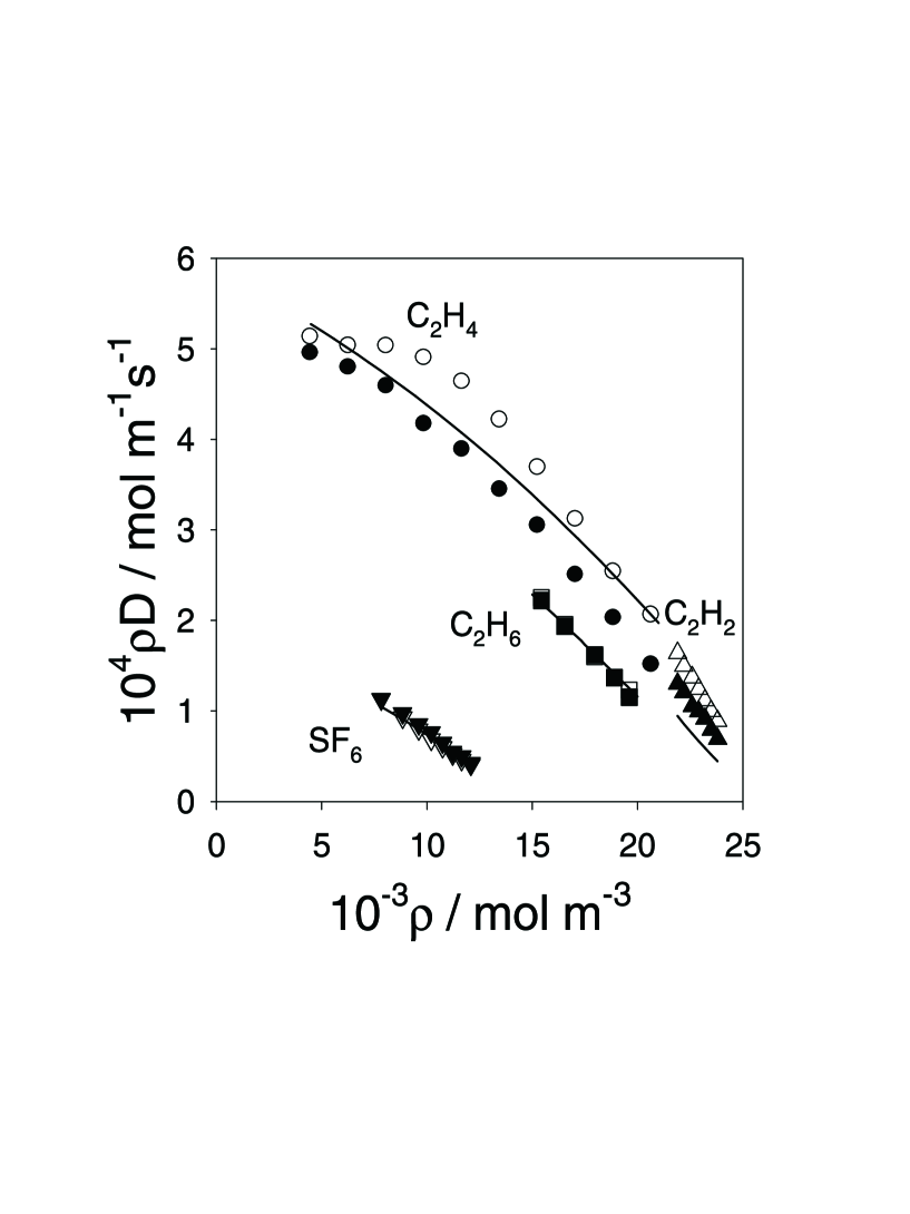
Figure 2 shows the results for the product of density and self-diffusion coefficient of C2H6, C2H4, C2H2, and SF6 compared to experimental data [41, 42, 43, 44] and Liu’s correlation. For C2H6 and C2H4 the considered state points lie in the homogeneous liquid region at temperatures of 273 K and 298.15 K, respectively. For C2H2 and SF6 the states correspond to the saturated liquid, the C2H2 densities were taken from Ref. 45. Good agreement with the experimental data is found. The best results are found for C2H6 and SF6 with average deviations of only 2% and 6%. For C2H2, the predictions of the simulation are too low by about 20%, for C2H4 they are also too low by about 15%. The experimental data of C2H4 show a pronounced curvature that is neither reproduced by the simulations nor by Liu’s correlation. Liu’s correlation is as good as the simulation for SF6 and C2H6, worse than the simulation for C2H2, but slightly better for C2H4.
To study the dependence of the self-diffusion coefficient on the number of particles, one state point for N2 at =85 K, =27.526 103 mol m-3 was chosen. For this state point, a sequence of simulations with increasing number of particles: =108, 256, 500, 864, and 1372 was carried out. The values for the self-diffusion coefficients were 3.78(6), 3.96(5), 4.03(1), 4.13(2), 4.21(2) in 109m s-1, respectively. An estimate of the self-diffusion coefficient for an infinite system size can be obtained by a linear fit of the self-diffusion coefficient data as a function of the inverse box length [46]. This fit yields a value of 4.50(4) 10-9 m s-1 for an infinitely large system, that is about 10% larger than the results with =500 particles. As most predictions of self-diffusion coefficients are below the experimental data, the finite-size correction can improve the agreement with the experimental data for most fluids. Exceptions are F2, SF6, and C2H6, for which the deviations would increase.
3.2. Binary Maxwell-Stefan Diffusion Coefficients
In this section, the results obtained for the binary mixtures N2+CO2, N2+C2H6, and CO2+C2H6 at 253.15 K and 20 MPa are presented. Numerical data are given in Table III, self-diffusion coefficients of pure fluids in binary mixtures are reported with statistical uncertainties less than 1%; binary MS diffusion coefficients are reported with statistical uncertainties of about 10%. These mixtures were selected since their vapor-liquid equilibria were successfully calculated with the present molecular models [22]. The simulated MS diffusion coefficients are compared with the predictions from the equations of Darken, Caldwell and Babb, and Vignes, cf. Eqs. (7), (8), and (9). To evaluate their performance, the average relative deviation, , was calculated. Experimental data for comparison are unfortunately not available. The input needed for Eqs. (7) to (9) were therefore simulation data, i.e. self-diffusion coefficients for Darken’s equation and infinite dilution diffusion coefficients for the equations of Caldwell and Babb and of Vignes.
Figure 3 shows the results for the binary MS diffusion coefficients for the mixture N2+CO2 compared to the equations of Caldwell and Babb, Darken, and Vignes. The MS diffusion coefficient increases as the mole fraction of N2 increases due to the smaller size and mass of the N2 molecule. The simulation results lie above the linear interpolation between the infinite dilution diffusion coefficients, i.e. Caldwell and Babb’s equation. Vignes’ equation gives a different behavior, with negative deviations from the linear interpolation, whereas Darken’s equation predicts positive deviations from the linear interpolation for high N2 mole fractions and negative deviations for low mole fractions.
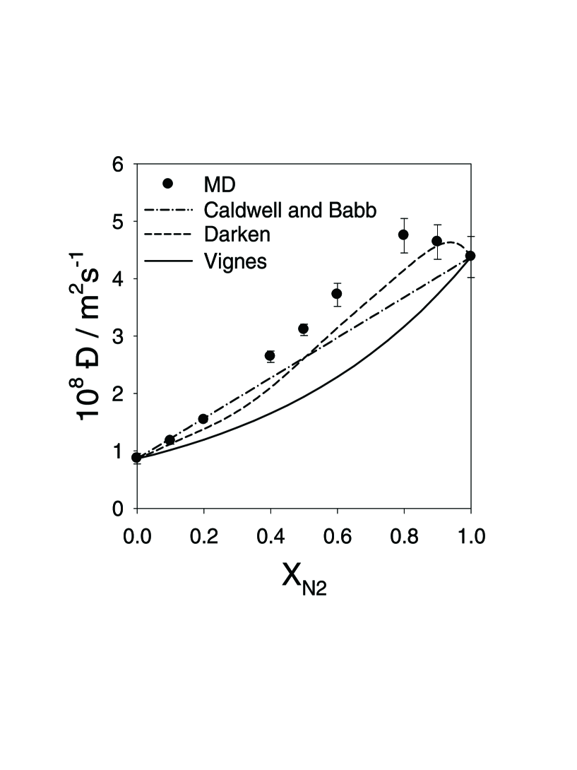
Figure 4 shows the results for the binary MS diffusion coefficients of the mixture N2+C2H6. In this case, the MS diffusion coefficients lie below the linear interpolation of the infinite dilution diffusion coefficients for mole fractions smaller than 0.5 and lie above the linear interpolation for mole fractions larger than 0.5. The results of Darken’s equation agree well with the simulation data. The average deviation is only about 6%. The equation of Vignes fails to reproduce the shape of the curve, which results in an average deviation of about 20%. The deviations between the simulation results and the correlation of Caldwell and Babb are also about 20%.
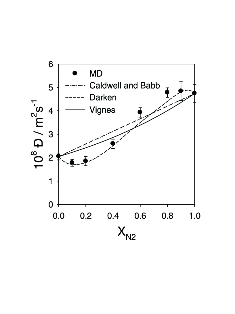
Figure 5 shows the results for the binary MS diffusion coefficients of the mixture CO2+C2H6. In this case, the MS diffusion coefficients lie above the linear interpolation between the infinite dilution diffusion coefficients (Caldwell and Babb) over the whole composition range. Also, Darken’s equation here yields the best results with an average deviation of 12%, whereas the equations of Caldwell and Babb and of Vignes yield deviations of 23% and 28%, respectively. Again Vignes’ equation does not reproduce the sign of the deviations from the linear interpolation correctly.
Figures 3, 4, and 5 show that the
curvature of the MS diffusion coefficient is a function of the
mole fraction, depending qualitatively on the mixture. It
can be concave, with a positive deviation from the linear course,
or convex with a negative deviation, or both. The investigated
mixtures are not strongly polar, and also in the 2CLJQ models only
quadrupolar interactions are present. However, the MS diffusion
coefficients of these mixtures can not be well represented by the
equations of Caldwell and Babb or of Vignes, that are often claimed
to be adequate for such simple mixtures
[18].
Dullien [47] compared the predictions of Vignes’
equation with experimental data, and also found that in many
cases, where the mixtures were nonassociating, the
equation of Vignes was not able to predict the binary MS diffusion
coefficients correctly. The equation of Darken shows the best performance in
all cases. That is due to the fact that it uses more information
than the other two. Moreover, it can be shown that it is exact if
the cross correlations between different particles of the same
species and particles of different species are neglected
[5]. Unfortunately, Darken’s equation is of little
use for most practical applications.
3.3. Binary Self-diffusion Coefficients
Figures 6-8 show the results for self-diffusion coefficients of the pure components in the mixtures N2+CO2, N2+C2H6, and CO2+C2H6 at 253.15 K and 20 MPa, together with those for the binary MS diffusion coefficients. Whereas for N2+CO2 and N2+C2H6 the MS diffusion coefficients can qualitatively be described by a simple interpolation as indicated by Darken’s equation. The situation is different for CO2+C2H6, cf. Fig. 8. The self-diffusion coefficients are almost equal for that mixture at all compositions. Nevertheless, the MS diffusion coefficient from the simulations is larger so that Eq. (7) is inappropriate.
4. CONCLUSION
In the present work, molecular dynamics simulation and the
Green-Kubo formalism were used to calculate self- and binary MS
diffusion coefficients for a class of fluids modeled by the 2CLJQ
intermolecular potential. The potential parameters were taken from previous work
[15, 22]
where they were adjusted to experimental vapor-liquid equilibria only.
Eight pure fluids, i.e. F2, N2,
CO2, CS2, C2H6, C2H4, C2H2 and three
binary mixtures, i.e. N2+CO2, N2+C2H6 and
CO2+C2H6, were studied. Self-diffusion coefficients
are reported with statistical uncertainties smaller than 1%. These results do not consider
corrections due to the long-time tail, the error due to it
is estimated to be about 3%. Deviations between the predicted and the experimental data do not exceed 20%.
The correction due to the finite size of the simulated system increases the
self-diffusion coefficients typically by 10%. With this correction an even better
agreement can be expected for most fluids. Exceptions are F2, SF6, and C2H6
for which the deviations would increase.
For the binary mixtures, predictions from the simulations are only compared to results from the equations of Darken, Caldwell and Babb, and Vignes, as experimental data were not available. The self-diffusion coefficients are reported with statistical uncertainties smaller than 1% and the binary MS diffusion coefficients are reported with statistical uncertainties of about 10%. In agreement with previous findings [8], Darken’s equation yields the best agreement in all cases with average deviations of only 10%. Unfortunately, this equation requires self-diffusion coefficients in the mixture as input data. The two simple equations of Caldwell and Babb and of Vignes which use infinite dilution diffusion coefficients as input data, fail to predict the shape of the composition dependence of the MS diffusion coefficients, which shows a strong curvature, despite the fairly simple molecules studied here. This indicates that more accurate correlations for the prediction of MS diffusion coefficients are needed. For their development, molecular simulation is a useful tool, as it can relate molecular properties, i.e. polarity, anisotropy etc., to diffusion coefficients.
| Fluid | / (Å) | /kB / (K) | L / (Å) | 1020Q /(C m2) | / (g mol-1) |
|---|---|---|---|---|---|
| 2.8258 | 52.147 | 1.4129 | 2.9754 | 38.00 | |
| 3.3211 | 34.897 | 1.0464 | 4.8024 | 28.01 | |
| 2.9847 | 133.22 | 2.4176 | 12.6549 | 44.01 | |
| 3.6140 | 257.68 | 2.6809 | 13.0081 | 76.14 | |
| 3.4896 | 136.99 | 2.3762 | 2.7609 | 30.07 | |
| 3.7607 | 76.950 | 1.2695 | 14.4468 | 28.05 | |
| 3.5742 | 79.890 | 1.2998 | 16.9218 | 28.05 | |
| 3.9615 | 118.98 | 2.6375 | 26.7074 | 146.06 |
| 10-3 | 109 | 109 | 10-3 | 109 | 109 | |||
| (K) | (mol m-3) | (m2 s-1) | (m2 s-1) | (K) | (mol m-3) | (m2 s-1) | (m2 s-1) | |
| 54.0 | 44.824 | 0.569 | 0.569(2) | 77.0 | 28.861 | 2.526 | 2.923(8) | |
| 62.0 | 43.497 | 1.05 | 0.905(2) | 80.0 | 28.380 | 2.996 | 3.309(5) | |
| 70.0 | 42.166 | 1.69 | 1.361(3) | 83.0 | 27.870 | 3.509 | 3.757(8) | |
| 78.0 | 40.787 | 2.46 | 1.903(6) | 85.0 | 27.526 | 3.875 | 4.03(1) | |
| 88.0 | 38.968 | 3.57 | 2.793(8) | 88.0 | 27.006 | 4.459 | 4.63(1) | |
| 96.0 | 37.405 | 4.55 | 3.575(6) | 90.0 | 26.643 | 4.871 | 4.93(1) | |
| 105.0 | 35.497 | 5.73 | 4.74(1) | 93.0 | 26.079 | 5.522 | 5.54(1) | |
| 273.0 | 21.102 | 13.50 | 10.41(3) | 298.15 | 4.4955 | 113.6 | 110.0(3) | |
| 273.0 | 21.453 | 13.00 | 10.39(6) | 298.15 | 6.2923 | 79.91 | 76.1(3) | |
| 273.0 | 22.333 | 11.70 | 9.274(3) | 298.15 | 8.0927 | 62.10 | 56.6(1) | |
| 273.0 | 23.046 | 10.70 | 8.156(4) | 298.15 | 9.8895 | 49.45 | 42.1(2) | |
| 273.0 | 23.460 | 10.00 | 7.890(2) | 298.15 | 11.690 | 39.58 | 33.20(8) | |
| 273.0 | 23.900 | 9.50 | 7.518(4) | 298.15 | 13.487 | 31.21 | 25.5(1) | |
| 298.15 | 15.283 | 24.08 | 19.90(7) | |||||
| 298.15 | 17.084 | 18.20 | 14.60(3) | |||||
| 298.15 | 18.881 | 13.44 | 10.70(3) | |||||
| 298.15 | 20.681 | 9.927 | 7.28(9) | |||||
| 273.0 | 15.431 | 14.6 | 14.40(4) | 298.2 | 16.489 | 4.26 | 3.209(7) | |
| 273.0 | 16.550 | 11.8 | 11.71(6) | 298.2 | 17.019 | 3.64 | 2.653(8) | |
| 273.0 | 17.968 | 8.91 | 9.008(4) | 298.2 | 17.514 | 3.21 | 2.264(7) | |
| 273.0 | 18.902 | 7.24 | 7.230(2) | 298.2 | 18.031 | 2.61 | 1.867(5) | |
| 273.0 | 19.609 | 6.27 | 5.870(1) | 298.2 | 18.543 | 2.23 | 1.532(5) | |
| 192.0 | 23.754 | 3.74 | 2.91(1) | 240.0 | 12.091 | 3.35 | 3.52(3) | |
| 197.0 | 23.463 | 4.26 | 3.37(1) | 250.0 | 11.653 | 3.94 | 4.28(2) | |
| 202.0 | 23.167 | 4.82 | 3.95(1) | 260.0 | 11.221 | 4.66 | 4.89(4) | |
| 207.0 | 22.863 | 5.43 | 4.35(1) | 270.0 | 10.742 | 5.59 | 6.03(2) | |
| 212.0 | 22.554 | 6.07 | 4.66(1) | 280.0 | 10.201 | 6.71 | 7.49(4) | |
| 217.0 | 22.237 | 6.76 | 5.44(1) | 290.0 | 9.606 | 8.29 | 8.87(5) | |
| 222.0 | 21.912 | 7.49 | 5.95(2) | 300.0 | 8.846 | 10.5 | 11.00(2) | |
| 310.0 | 7.826 | 14.4 | 14.50(5) |
| 10-3 | 109 | 109 | 109 | |
| (mol m-3) | (m2 s-1) | (m2 s-1) | (m2 s-1) | |
| 0.0 | 24.08 | 8.7(9) | 6.86(2) | 8.7(9) |
| 0.1 | 22.96 | 11.57(7) | 8.40(3) | 11.7(5) |
| 0.2 | 21.47 | 14.60(7) | 10.55(4) | 15.4(3) |
| 0.4 | 17.73 | 24.13(10) | 16.74(2) | 26(1) |
| 0.5 | 15.59 | 30.77(8) | 21.19(7) | 31(1) |
| 0.6 | 13.60 | 38.63(6) | 26.83(19) | 37(2) |
| 0.8 | 10.90 | 53.87(20) | 38.39(25) | 47(3) |
| 0.9 | 9.968 | 61.25(20) | 44.08(24) | 46(3) |
| 1.0 | 9.356 | 67.49(13) | 43(4) | 43(4) |
| 0.0 | 13.87 | 20(1) | 11.97(4) | 20(1) |
| 0.1 | 13.85 | 17.39(9) | 13.27(2) | 18(1) |
| 0.2 | 13.74 | 19.58(16) | 14.98(4) | 18(1) |
| 0.4 | 12.91 | 26.48(6) | 19.81(11) | 26(2) |
| 0.6 | 11.21 | 42.88(50) | 31.18(20) | 39(3) |
| 0.8 | 9.302 | 54.42(11) | 40.25(38) | 48(4) |
| 0.9 | 8.566 | 62.88(17) | 47.08(40) | 48(4) |
| 1.0 | 8.059 | 70.21(20) | 47(4) | 47(4) |
| 0.0 | 16.10 | 13(1) | 11.84(1) | 13(1) |
| 0.1 | 16.47 | 12.38(14) | 11.75(6) | 13(1) |
| 0.2 | 16.88 | 11.98(5) | 11.64(6) | 13(1) |
| 0.4 | 17.95 | 10.93(6) | 11.09(8) | 13(1) |
| 0.6 | 19.49 | 9.63(4) | 10.08(6) | 12(1) |
| 0.8 | 21.59 | 8.09(3) | 8.66(9) | 10.3(8) |
| 0.9 | 22.94 | 7.21(1) | 7.78(14) | 8.2(7) |
| 1.0 | 24.66 | 6.15(6) | 5.1(7) | 5.1(7) |


REFERENCES
1. B.J. Alder and T.E. Wainwright, Phys. Rev. A 18:988 (1967).
2. B.J. Alder and T.E. Wainwright, Phys. Rev. A 1:18 (1970).
3. G. Jaccuci and I.R. Mcdonald, Physica A 80:607 (1975).
4. D. Jolly and R. Bearman, Mol. Phys. 41:137 (1980).
5. M. Schoen and C. Hoheisel, Mol. Phys. 52:33 (1984).
6. J.M. Stoker and R.L. Rowley, J. Chem. Phys. 91:3670 (1989).
7. R.L. Rowley and J.M. Stoker, Int. J. Thermophys. 12:501 (1991).
8. G.A. Fernández, J. Vrabec, and H. Hasse, Int. J. Thermophys. 25:175 (2004).
9. G.A. Fernández, J. Vrabec, and H. Hasse, Fluid Phase Equilib. 221:157 (2004).
10. I.R. McDonald and K. Singer, Mol. Phys. 23:29 (1972).
11. P.S.Y. Cheung and J.G. Powles, Mol. Phys. 30:921 (1975).
12. R. Vogelsang and C. Hoheisel, Phys. Chem. Liq. 16:189 (1987).
13. C. Hoheisel, Mol. Phys. 62:239 (1987).
14. D. Möller and J. Fischer, Fluid Phase Equilib. 100:35 (1994).
15. J. Vrabec, J. Stoll, and H. Hasse, J. Phys. Chem. B 105:12126 (2001).
16. C.S. Caldwell and A.L. Babb, J. Phys. Chem. 60:51 (1956).
17. L.S. Darken, Trans. Am. Inst. Mining Metall. Eng. 175:184 (1948).
18. A. Vignes, Ind. Eng. Chem. Fundam. 5:189 (1966).
19. C.G. Gray, and K.E. Gubbins, Theory of Molecular Fluids, Vol. 1: Fundamentals, (Clarendon Press, Oxford, 1984).
20. J. Vrabec and J. Fischer, AIChE J. 43:212 (1996).
21. J. Vrabec, J. Stoll, and H. Hasse, Mol. Sim. 31:215 (2005).
22. J. Stoll, J. Vrabec, and H. Hasse, AIChE J. 49:2187 (2003).
23. M.S. Green, J. Chem. Phys. 22:398 (1954).
24. R. Kubo, J. Phys. Soc. Japan 12:570 (1957).
25. R. Zwanzig, Ann. Rev. Phys. Chem. 16:67 (1965).
26. C. Hoheisel, Phys. Rep. 245:111 (1994).
27. NIST Chemistry WebBook, http://webbook.nist.gov/chemistry.
28. R. Lustig, Mol. Phys. 65:175 (1988).
29. J.M. Haile, Molecular Dynamics Simulation (John Wiley & Sons Inc., New York, 1997).
30. S. Nosé, Mol. Phys. 100:191 (2002).
31. D. Frenkel and R. Smit, Understanding Molecular Simulation (Academic Press, San Diego, 1996).
32. H.C. Andersen, J. Chem. Phys. 72:2384 (1980).
33. D. Fincham, N. Quirke, and D.J. Tildesley, J. Chem. Phys. 84:4535 (1986).
34. H. Liu, C.M. Silva, and E.A. Macedo, Chem. Eng. Sci. 53:2403 (1998).
35. D.E. O’Reilly, E.M. Peterson, D.I. Hogenboom, and C.E. Scheie, J. Chem. Phys. 54:4194 (1971).
36. K. Krynicki, E.J., Rahkamaa, and J.P. Powles, Mol. Phys. 28:853 (1974).
37. P.E. Etesse, J.A. Zega, and R. Kobayashi, J. Chem. Phys. 97:2022 (1992).
38. L.A. Woolf, J. Chem. Soc. Faraday Trans. 1 78:583 (1982).
39. N.B. Vargaftik, Y.K. Vinogradov, and V.S. Yargin, Handbook of Physical Properties of Liquids and Gases (Begell House, New York, 1996).
40. E.W. Lemmon, M.O. McLinden, and M.L. Huber, REFPROP (NIST Standard Reference Database 23, Version 7.0, 2002).
41. A. Greiner-Schmid, S. Wappmann, M. Has, and H.D. Lüdemann, J. Chem. Phys. 94:5643 (1991).
42. B. Arends, K.O. Prins, and N.J. Trappeniers, Physica A 107A:307 (1981).
43. C.E. Scheie, E.M. Peterson, and D.E. O’Reilly, J. Chem. Phys. 59:2303 (1973).
44. J.K. Tison and E.R. Hunt, J. Chem. Phys. 54:1526 (1971).
45. T.E. Daubert and R.P. Danner, Data compilation tables of properties of pure
substances, AIChE (American Chemical Society, New York, 1985).
46. Yeh, I. and G. Hammer, J. Chem. Phys. 108:158 (2004).
47. F.A.L. Dullien, Ind. Eng. Chem. Fundam. 10:41 (1971).
References
- [1] B.J. Alder and T.E. Wainwright, Phys. Rev. A. 18:988 (1967).
- [2] B.J. Alder and T.E. Wainwright, Phys. Rev. A. 1:18 (1970).
- [3] G. Jaccuci and I.R. Mcdonald, Physica A 80:607 (1975).
- [4] D. Jolly and R. Bearman, Mol. Phys. 41:137 (1980).
- [5] M. Schoen and C. Hoheisel, Mol. Phys. 52:33 (1984).
- [6] J.M. Stoker and R.L. Rowley, J. Chem. Phys. 91:3670(1989).
- [7] R.L. Rowley and J.M. Stoker, Int. J. Thermopys.12:501(1991).
- [8] G.A. Fernández, J. Varbec, and H. Hasse Int. J. Thermopys.25:175(2004).
- [9] G.A. Fernández, J. Varbec, and H. Hasse Fluid Phase Equilib.221:157(2004).
- [10] I.R. McDonald, K. Singer, Mol. Phys. 23:29(1972).
- [11] P.S.Y. Cheung, and J.G. Powles, Mol. Phys. 30:921(1975).
- [12] R. Vogelsang, and C. Hoheisel, Phys. Chem. Liq 16:189-203(1987).
- [13] C. Hoheisel, Mol. Phys. 62:239(1987).
- [14] D. Möller and J. Fischer, Fluid Phase Equilib. 100:35(1994).
- [15] J. Vrabec, J. Stoll and H. Hasse, J. Phys. Chem. B 105:12126(2001).
- [16] C.S. Caldwell and A.L. Babb, J. Phys. Chem. 60:51(1956).
- [17] L.S. Darken, AIME 175:184 (1948).
- [18] A. Vignes, Ind. Eng. Chem. Fundam. 2:189(1966).
- [19] C.G. Gray, and K.E. Gubbins,Theory of Molecular Fluids, Vol. 1: Fundamentals, (Clarendon Press, Oxford, 1984).
- [20] J. Vrabec, J. Stoll, and H. Hasse, J. Phys. Chem. B submitted.
- [21] J. Vrabec and J. Fischer, AiChe J. 43:212(1996).
- [22] J. Stoll, J. Vrabec, and H. Hasse, AiChe J. 49:2187(2003).
- [23] M.S. Green, J. Chem. Phys. 22:398(1954).
- [24] R. Kubo, J. Phys. Soc. Japan 12:570(1957).
- [25] R. Zwanzig, Ann. Rev. Phys. Chem. 16:67(1965).
- [26] C. Hoheisel, Phys. Rep. 245:111(1994).
- [27] NIST Chemistry WebBook, http://webbook.nist.gov/chemistry.
- [28] R. Lustig, Mol. Phys. 65:175(1988).
- [29] J.M. Haile, Molecular Dynamics Simulation(John Wiley & Sons Inc., New York, 1997).
- [30] S. Nosé, Mol. Phys. 100:191(2002).
- [31] D. Frenkel and R. Smit, Understanding Molecular Simulation (Academic Press, San Diego, 1996).
- [32] H.C. Andersen, J. Chem. Phys. 72:2384(1980).
- [33] D. Fincham, N. Quirke, and D.J. Tildesley, J. Chem. Phys. 84:4535(1986).
- [34] H. Liu, C.M. Silva, and E.A. Macedo, Chem. Eng. Sci. 53:2403 (1998).
- [35] D.E. O’Reilly, E.M. Peterson, D.I. Hogenboom, and C.E. Scheie, J. Chem. Phys. 54:4194(1971).
- [36] K. Krynicki, E.J., Rahkamaa, and J.P. Powles, Mol. Phys. 28:853(1974).
- [37] P.E. Etesse, J.A. Zega, and R. Kobayashi, J. Chem. Phys. 97:2022(1992).
- [38] L.A. Woolf, J. Chem. Soc. Faraday. Trans. 1 78:583(1982).
- [39] N.B. Vargaftik, Y.K. Vinogradov, and V.S. Yargin, Handbook of Physical Properties of Liquids and Gases(Begell house, inc., New York, 1996).
- [40] E.W. Lemmon, M.O. McLinden, and M.L. Huber, REFPROP(NIST Standard reference Database 23, Version 7.0, 2002).
- [41] A. Greiner-Schmid, S. Wappmann, M. Has, and H.D. Lüdemann, J. Chem. Phys. 94:5643(1991).
- [42] B. Arends, K.O. Prins, and N.J. Trappeniers, Physica A 107A:307(1981).
- [43] C.E. Scheie, E.M. Peterson, and D.E. O’Reilly, J. Chem. Phys. 59:2303(1973).
- [44] J.K. Tison, and E.R. Hunt, J. Chem. Phys. 54:1526(1971).
- [45] T.E. Daubert,and R.P. Daner, Data compilation tables of properties of pure subtances, AIChE,(American Chemical Society, New York, 1985).
- [46] Yeh, I. and G. Hammer, J. Chem. Phys. 108:158(2004).
- [47] F.A.L. Dullien, Ind. Eng. Chem. Fundam. 10:41(1971).