A Two-field Dilaton Model of Dark Energy

Abstract

We investigate the cosmological evolution of a two-field model of dark energy where one is a dilaton field with canonical kinetic energy and the other is a phantom field with a negative kinetic energy term. A phase-plane analysis shows that the phantom-dominated scaling solution is the stable late-time attractor of this type of models. We find that during the evolution of the universe, the equation of state $w$ changes from $w>-1$ to $w<-1$, which is consistent with the recent observations.

I Introduction

In recent years, observations of Type Ia supernovae (SNe Ia) [1, 2], cosmic microwave background (CMB) fluctuations [3, 4], and large-scale structures (LSS) [5, 6] indicate that the Universe is accelerating, therefore some form of dark energy whose fractional energy density is about $\Omega_{DE}=0.70$ must exist in the Universe to drive this acceleration. Dark energy has been one of the most active fields in modern cosmology since the discovery of accelerated expansion of our universe. Investigation on the nature of dark energy becomes one of the most important tasks for modern physics and modern astrophysics. Up to now, many candidates of dark energy have been proposed to fit various observations which include the simplest one, the Einstein’s cosmological constant [7], or a dynamical scalar field, such as quintessence [8], phantom [9], k-essence [10], tachyon [11] and so on. The present data seem to slightly favor an evolving dark energy with the equation-of-state parameter (EoS) $w<-1$ around present epoch and $w>-1$ in the near past. Obviously, $w$ cannot cross $-1$ for quintessence or phantom alone. Some efforts have been made to build dark energy model whose EoS can cross the phantom divide. In a universe filled with quintessence and phantom fields this case can be realized easily. This implement of dark energy, called as quintom, has been first proposed in Ref. [12], where the quintom model with an exponential potential and the existence, stability of cosmological scaling solutions in the context of spatially homogeneous cosmological models have been investigated. Phase-plane analysis of the spatially flat FRW models shows that the phantom-dominated scaling solution is the unique late-time attractor and there exists a transition from $w>-1$ to $w<-1$ [13]. Wei and Cai [14] suggested a hessence model, in which a non-canonical complex scalar field plays the role of dark energy. The cosmological evolution of the hessence dark energy is also investigated; it is found that the big rip never appears in the hessence model even in the most general case while beyond particular potentials and interaction forms.

The action of dilaton field in the presence of Einstein’s cosmological constant has been derived in Ref. [15]. The potential is the counterpart of the Einstein’s cosmological constant in the dilaton gravity theory. Since it can be reduced to the Einstein cosmological constant when the dilaton field is set to zero, the dilaton potential is called the cosmological constant term in the dilaton gravity theory. Compared to the ordinary scalar field, the action for phantom scalar field has only a sign difference before the kinetic term. Later, the explicit expression of the phantom potential have been given in Ref. [16]. A model of the Universe dominated by the dilaton field with a Liouville type potential has been presented in Ref. [17].

In this Letter, we investigate the cosmological evolution of a two-field model of dark energy where one is a dilaton field with canonical kinetic energy and the other is a phantom field with a negative kinetic energy term with Liouville type potentials.

II Equations of motion for the two-field Dilaton model

Let us start from a 4-dimensional theory in which gravity is coupled to dilaton and Maxwell field with an action:

$$S_{1}=\int d^{4}x\sqrt{-g}\left(R-2\partial_{\mu}\phi\partial^{\mu}\phi-V_{1}(\phi)+e^{-2\alpha\phi}F^{2}\right),$$ (1)

where R is the scalar curvature, $F^{2}=F_{\mu\nu}F^{\mu\nu}$ is the usual Maxwell contribution, $\alpha$ is an arbitrary constant governing the strength of the coupling between the dilaton and the Maxwell field, $V_{1}(\phi)$ is a potential of dilaton $\phi$ which is given by Ref. [15]

$$V_{1}(\phi)=\frac{2\lambda}{3(1+\alpha^{2})}[\alpha^{2}(3\alpha^{2}-1)e^{-\frac{2}{\alpha}\phi}+(3-\alpha^{2})e^{2\alpha\phi}+8\alpha^{2}e^{(\alpha-\frac{1}{\alpha})\phi}],$$ (2)

here $\lambda$ is the cosmological constant. One can verify that the potential reduces to the Einstein cosmological constant when $\alpha=0$ or $\phi=0$. Compared to the action of the ordinary scalar fields, the phantom field has one negative kinetic term. In order to obtain a real action of the Einstein-Maxwell field in the presence of the phantom, we can make substitutions in the action as follows Ref. [16]

$$\phi\to i\psi,\alpha\to i\beta,$$ (3)

where $i$ is the imaginary unit. Thus we get the action

$$S_{2}=\int d^{4}x\sqrt{-g}\left(R+2\partial_{\mu}\psi\partial^{\mu}\psi-V_{2}(\psi)+e^{-2\beta\psi}F^{2}\right),$$ (4)

and the potential for the phantom field

$$V_{2}(\psi)=\frac{2\lambda}{3(1-\beta^{2})}[\beta^{2}(3\beta^{2}+1)e^{-\frac{2}{\beta}\psi}+(\beta^{2}+3)e^{2\beta\psi}-8\beta^{2}e^{(\beta-\frac{1}{\beta})\psi}].$$ (5)

One can also verify that, when $\beta=0$ or $\psi=0$ the action reduces to the Einstein-Maxwell action and when $F^{2}=0$ the action reduces to the Einstein-phantom action.

We consider the action in a simple model which contains a normal scalar field $\phi$ and a negative-kinetic scalar field $\psi$, assuming that there is no direct coupling between the phantom field and the normal scalar field with such potentials,

$$S=\int d^{4}x\sqrt{-g}\left(R-2\partial_{\mu}\phi\partial^{\mu}\phi+2\partial_{\mu}\psi\partial^{\mu}\psi-V_{1}(\phi)-V_{2}(\psi)+\mathcal{L_{\textrm{m}}}\right),$$ (6)

where $\mathcal{L_{\textrm{m}}}$ represents the Lagrangian density of matter fields. Considering a flat Universe which is described by the Friedmann-Robertson-Walker metric, the homogeneous fields $\phi$ and $\psi$ can be described by a fluid with an effective energy density $\rho$ and an effective pressure $P$ given by

$$\rho = \dot{\phi}^{2}-\dot{\psi}^{2}+\frac{1}{2}V_{1}(\phi)+\frac{1}{2}V_{2}(\psi),$$ (7)

$$P = \dot{\phi}^{2}-\dot{\psi}^{2}-\frac{1}{2}V_{1}(\phi)-\frac{1}{2}V_{2}(\psi).$$ (8)

The corresponding equation of state (EoS) parameter is given by

$$w=\frac{\dot{\phi}^{2}-\dot{\psi}^{2}-\frac{1}{2}V_{1}(\phi)-\frac{1}{2}V_{2}(\psi)}{\dot{\phi}^{2}-\dot{\psi}^{2}+\frac{1}{2}V_{1}(\phi)+\frac{1}{2}V_{2}(\psi)}.$$ (9)

Then the equations of motion for the fields and the Friedmann equation can be written as

$$\ddot{\phi} = -3H\dot{\phi}-\frac{1}{4}\frac{dV_{\phi}(\phi)}{d\phi},$$ (10)

$$\ddot{\psi} = -3H\dot{\psi}+\frac{1}{4}\frac{dV_{\psi}(\psi)}{d\psi},$$ (11)

$$3H^{2} = \kappa^{2}\left(\dot{\phi}^{2}-\dot{\psi}^{2}+\frac{1}{2}V_{1}(\phi)+\frac{1}{2}V_{2}(\psi)+\rho_{\gamma}\right),$$ (12)

where $\rho_{\gamma}$ is the density of fluid with a barotropic equation of state $P_{\gamma}=(\gamma-1)\rho_{\gamma}$ with $\gamma$ a constant and $0<\gamma\leq 2$ ($\gamma=4/3$ for radiation and $\gamma=1$ for dust mater). The equation (12) is the Friedmann constraint equation.

III Phase space analysis and the critical points

In this section, we investigate the two-field Dilaton model via the conventional phase space analysis. Similar as in Ref. [18], we define the following new dimensionless variables

$$x_{\phi}\equiv\frac{\kappa\dot{\phi}}{\sqrt{3}H} \quad y_{\phi}\equiv\frac{\kappa\sqrt{V_{1}(\phi)}}{\sqrt{6}H},\quad\lambda_{\phi}\equiv\frac{\sqrt{3}\frac{\partial_{1}(\phi)}{\partial\phi}}{\kappa V_{1}(\phi)},\quad\Gamma_{\phi}\equiv\frac{V_{1}(\phi)\frac{\partial^{2}V_{1}(\phi)}{\partial^{2}\phi}}{[\frac{\partial V_{1}(\phi)}{\partial\phi}]^{2}},$$ ,

$$x_{\psi}\equiv\frac{\kappa\dot{\psi}}{\sqrt{3}H} \quad y_{\psi}\equiv\frac{\kappa\sqrt{V_{2}(\psi)}}{\sqrt{6}H},\quad\lambda_{\psi}\equiv\frac{\sqrt{3}\frac{\partial_{1}(\psi)}{\partial\psi}}{\kappa V_{2}(\psi)},\quad\Gamma_{\psi}\equiv\frac{V_{1}(\psi)\frac{\partial^{2}V_{1}(\psi)}{\partial^{2}\psi}}{[\frac{\partial V_{2}(\psi)}{\partial\psi}]^{2}},$$ ,

$$z\equiv\frac{\kappa\sqrt{\rho_{\gamma}}}{\sqrt{6}H},$$

the equations of motion (10)-(12) can be rewritten as the following system of equations:

$$\frac{dx_{\phi}}{dN} = 3x_{\phi}\left(x_{\phi}^{2}-x_{\psi}^{2}+\frac{\gamma}{2}z^{2}-1\right)+\frac{1}{2}\lambda_{\phi}y_{\phi}^{2}\,,$$ (13)

$$\frac{dy_{\phi}}{dN} = 3y_{\phi}\left(x_{\phi}^{2}-x_{\sigma}^{2}+\frac{\gamma}{2}z^{2}\right)-\frac{1}{2}\lambda_{\phi}x_{\phi}y_{\phi}\,,$$ (14)

$$\frac{d\lambda_{\phi}}{dN} = -x_{\phi}\lambda_{\psi}\left(\Gamma_{\phi}-1\right),$$ (15)

$$\frac{dx_{\psi}}{dN} = 3x_{\psi}\left(x_{\phi}^{2}-x_{\psi}^{2}+\frac{\gamma}{2}z^{2}-1\right)-\frac{1}{2}\lambda_{\psi}y_{\psi}^{2}\,,$$ (16)

$$\frac{dy_{\psi}}{dN} = 3y_{\psi}\left(x_{\phi}^{2}-x_{\sigma}^{2}+\frac{\gamma}{2}z^{2}\right)-\frac{1}{2}\lambda_{\psi}x_{\psi}y_{\psi}\,,$$ (17)

$$\frac{d\lambda_{\psi}}{dN} = -x_{\psi}\lambda_{\psi}\left(\Gamma_{\psi}-1\right),$$ (18)

$$\frac{dz}{dN} = 3z\left(x_{\phi}^{2}-x_{\sigma}^{2}-\frac{\gamma}{2}z^{2}-\frac{\gamma}{2}\right),$$ (19)

where $N$ is the logarithm of the scale factor ($N\equiv\ln a$), and the Fridemann constraint equation (11) becomes

$$x_{\phi}^{2}+y_{\phi}^{2}-x_{\psi}^{2}+y_{\psi}^{2}+z^{2}=1.$$ (20)

Different from the case of a single exponential potential, the parameters $\lambda_{\phi,\psi}$ and $\Gamma$ here are variables of $\phi$ and $\psi$. Strictly speaking, the above system is not an autonomous system. Thus, if we want to discuss the phase plane, we need to find the constraints on the potential, or equivalently the conditions under which the potential may have the property we require in order that we can get some explicit results.

Critical points correspond to fixed points where $\frac{dx_{\phi}}{dN}=0$, $\frac{dy_{\phi}}{dN}=0$, $\frac{d\lambda_{\phi}}{dN}=0$, $\frac{dx_{\psi}}{dN}=0$, $\frac{dy_{\psi}}{dN}=0$, $\frac{d\lambda_{\psi}}{dN}=0$, $\frac{dz}{dN}=0$. Observing these equations, one can find that the physically meaningful critical points $(x_{\phi,c},y_{\phi,c},\lambda_{\phi,c},x_{\psi,c},y_{\psi,c},\lambda_{\psi,c})$ of the system are: (Note that we will restrict our discussion of the existence and stability of critical points in the expanding universes with $H>0$).

(i). $(\lambda_{\phi,c}\not=0,\ \lambda_{\psi,c}\not=0)$ could be fixed by $\Gamma_{\phi}=1,\ \Gamma_{\psi}=1$;

(ii). $(x_{\phi,c}=0,\ y_{\phi,c}^{2}+y_{\psi,c}^{2}=1,\ \lambda_{\phi,c}=0,\ x_{\psi,c}=0,\ \lambda_{\psi,c}=0)$;

(iii). $(x_{\phi,c}=0,\ y_{\phi,c}=0,\ \lambda_{\phi,c}=any,\ x_{\psi,c}=0,\ y_{\psi,c}=0,\ \lambda_{\psi,c}=any)$.

In the case of (i), when $\Gamma_{\phi}=1,\ \Gamma_{\psi}=1$, then $\lambda_{\phi,c}=\frac{2\sqrt{3}}{\kappa},\ \lambda_{\psi,c}=\frac{2\sqrt{3}}{\kappa}$ and the two-fields potentials are given by

$$V_{1}(\phi) = \lambda(e^{-\frac{2\phi}{\sqrt{3}}}+e^{\frac{2\phi}{\sqrt{3}}}),$$ (21)

$$V_{2}(\psi) = 2\lambda e^{-2\psi}.$$ (22)

Thus we can determine the important parameters of the dilaton field and the phantom field:

$$\alpha = \frac{1}{\sqrt{3}},\ \textrm{or}\ \ \sqrt{3};\ \textrm{and}\ \beta=1.$$

In this case, the equations (13)-(19) have one two-dimensional hyperbola (Type $A$) embedded in four-dimensional phase-space corresponding to kinetic-dominated solutions, with EoS $w=1$ and fractional energy density $\Omega_{\textrm{DE}}=1$; a fixed point (Type $B$) corresponding to a dilaton-dominated solution, with $w=-1+{2}/{3\kappa^{2}}$ and $\Omega_{\textrm{DE}}=1$; a fixed point (Type $C$) corresponding to a fluid-dilaton-dominated solution, with $w=0$ and $\Omega_{\textrm{DE}}={3}/{2\kappa^{2}}$; and a fixed point (Type $D$) corresponding to a phantom-dominated solution, with $w=-1-{2}/{3\kappa^{2}}$ and $\Omega_{\textrm{DE}}=1$ (listed in Table 1).

Type	$x_{\phi}$	$y_{\phi}$	$x_{\psi}$	$y_{\psi}$	$z$	$w$	$\Omega_{\textrm{DE}}$	Stability
$A$	$x_{\phi}^{2}-x_{\psi}^{2}=1$	0	$x_{\phi}^{2}-x_{\psi}^{2}=1$	0	0	1	1	unstable
$B$	$\frac{1}{\sqrt{3}\kappa}$	$\sqrt{(1-\frac{1}{3\kappa^{2}})}$	0	0	0	$-1+\frac{2}{3\kappa^{2}}$	1	unstable
$C$	$\frac{\sqrt{3}\kappa}{2}$	$\sqrt{\frac{3\kappa^{2}\gamma(2-\gamma)}{4}}$	0	0	$\sqrt{1-\frac{3\kappa^{2}\gamma}{2}}$	0	$\frac{3}{2\kappa^{2}}$	unstable
$D$	0	0	$-\frac{1}{\sqrt{3}\kappa}$	$\sqrt{(1+\frac{1}{3\kappa^{2}})}$	0	$-1-\frac{2}{3\kappa^{2}}$	1	stable

Table 1: The properties of the critical points in a spatially flat FRW universe containing a phantom field and a normal scalar field in the case of (i).

In order to study the stability of the critical points, using the Friedmann constraint equation (20) we can reduce Eqs.(13)-(19) to four independent equations. Substituting linear perturbations $x_{\phi}\to x_{\phi}+\delta x_{\phi}$, $y_{\phi}\to y_{\phi}+\delta y_{\phi}$, $x_{\psi}\to x_{\psi}+\delta x_{\sigma}$ and $y_{\psi}\to y_{\psi}+\delta y_{\psi}$ into the four independent equations, we obtain the equation of perturbations to the first-order:

$$\delta x_{\phi}^{\prime} = 3\left(3x_{\phi}^{2}-x_{\psi}^{2}+\frac{\gamma}{2}z^{2}-1\right)\delta x_{\phi}+\lambda_{\phi}y_{\phi}\delta y_{\phi}-6x_{\phi}x_{\phi}\delta x_{\psi},$$ (23)

$$\delta y_{\phi}^{\prime} = 3y_{\phi}\left(2x_{\phi}-\frac{1}{6}\lambda_{\phi}\right)\delta x_{\phi}+\left(x_{\phi}^{2}-x_{\psi}^{2}+\frac{\gamma}{2}z^{2}-1\right)\delta y_{\phi}-6x_{\phi}y_{\phi}\delta x_{\psi},$$ (24)

$$\delta x_{\psi}^{\prime} = 6x_{\phi}x_{\psi}\delta x_{\phi}-3\left(x_{\phi}^{2}-3x_{\psi}^{2}+\frac{\gamma}{2}z^{2}-1\right)\delta x_{\psi}-\lambda_{\psi}y_{\psi}\delta y_{\psi},$$ (25)

$$\delta y_{\psi}^{\prime} = 6x_{\phi}x_{\psi}\delta y_{\phi}+3y_{\phi}(-2x_{\phi}-\frac{1}{6}\lambda_{\psi})\delta x_{\psi}-3\left(3x_{\phi}^{2}-x_{\psi}^{2}+\frac{\gamma}{2}z^{2}-1\right)\delta y_{\psi}.$$ (26)

The linear perturbations of system (23)-(26) about each fixed point gives four eigenvalues. The theory of stability requires that the real part of all eigenvalues should be negative. So we have:

Type $A$ (the kinetic-dominated solution):

$$m_{1}=3,\quad m_{2}=0,\quad m_{3}=3(2-\gamma),\quad m_{4}=3(1\pm\frac{1}{\sqrt{3}\kappa}),$$

indicating that this solution is always unstable.

Type $B$ (the dilaton-dominated solution):

$$m_{1}=\frac{6}{\kappa^{2}},\quad m_{2}=m_{3}=\frac{6}{\kappa^{2}}-3\gamma,\quad m_{4}=\frac{12}{\kappa^{2}}-3,$$

indicating that this solution is also unstable.

Type $C$ (the fluid-dilaton-dominated solution):

$$m_{1}=\frac{3\gamma}{2},\quad m_{2}=\frac{3\gamma}{2}-3,\quad m_{3,4}=-\frac{3(2-\gamma)}{4}\left(1\pm\sqrt{1-\frac{8\gamma(\frac{2}{\kappa^{2}}-3\gamma)}{\frac{2}{\kappa^{2}}(2-\gamma)}}\right),\\$$

indicating that this solution is still unstable.

Type $D$ (the phantom-dominated solution):

$$m_{1}=-\frac{1}{\kappa^{2}},\quad m_{2}=m_{3}=-\frac{1}{\kappa^{2}}-3,\quad m_{4}=-\frac{2}{\kappa^{2}}-3\gamma,$$

indicating that this solution is stable.

In the case of (ii) $(x_{\phi,c}=0,\ y_{\phi,c}^{2}+y_{\psi,c}^{2}=1,\ \lambda_{\phi,c}=0,\ x_{\psi,c}=0,\ \lambda_{\psi,c}=0)$, the equations (13)-(19) have one fixed point Type $E$ embedded in six-dimensional phase-space which corresponds to eigenvalues $(-3,-3\gamma,0,0,0,0)$, $w=-1$ and $\Omega_{\textrm{DE}}=1$. This indicates that the critical point is a de Sitter attractor.

In the case of (iii) $(x_{\phi,c}=0,\ y_{\phi,c}=0,\ \lambda_{\phi,c}=any,\ x_{\psi,c}=0,\ y_{\psi,c}=0,\ \lambda_{\psi,c}=any)$, the equations (13)-(19) have one fixed point Type $F$ embedded in six-dimensional phase-space which corresponds to eigenvalues $(-3(\gamma-2)/2,-3\gamma/2,0,-3(\gamma-2)/2,-3\gamma/2,0)$, $w$ becomes meaningless and $\Omega_{\textrm{DE}}=0$. This indicates that the critical point is not a dynamical attractor.

IV Numerical Studies

Our numerical studies indicate that the EoS parameter $w$ changes from $>-1$ to $<-1$ as shown in Figure 1. We have assumed that there is no direct coupling between the phantom field and the normal scalar field in this paper. Without the loss of generality, the initial conditions $\phi(0),\ \psi(0),\ \dot{\phi}(0)$ and $\dot{\psi}(0)$ can be fixed in order to get the EoS today $(w=-1.02,\ a=1)$ [19], and the energy density of dark energy today $\Omega_{DE}=0.70$. The blue line represents the EoS of the two-field dilaton model, the black line represents the single dilaton model and the red line represents the single phantom model.

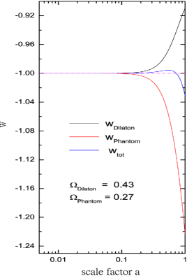
Figure 1: The evolution of the equation of state $w$ of the two-field dilaton model of dark energy. The blue line represents the EoS of the two-field model, the black line represents the single dilaton model and the red line represents the single phantom model.

V Conclusions and Discussions

In summary, we have investigated the possibility of constructing a two-field dark energy model which has the equation of state $w$ crossing $-1$ by using the dilaton and phantom fields. We have made a phase-space analysis of the evolution for a spatially flat FRW universe filled with a barotropic fluid and phantom-dilaton fields. It is shown that there exists the stable late-time attractor solution in the model. Also, we showed that the equation of state $w$ can cross $-1$ naturally. So the two-field dilaton field is a viable candidate for dark energy.

It is apparent that our model is also plagued with the instability problem at the quantum level which makes its existence doubtful. In fact, this is a common problem for nearly all phantom models. However, as argued by Carroll et al. [20], these models might be phenomenologically viable if considered as effective field theories valid only up to a certain momentum cutoff. According to their discussions, the instability timescale of the phantom quanta can be greater than the age of the universe provided that the cutoff is at or below 100 MeV. In this sense, the phantom quanta are stable against decay into gravitons and other particles. Therefore, considering astronomical observations favoring the phantom model for dark energy, it remains open if the phantom matter exists and acts as dark energy.

References

• (1) Riess A G et al. 1998 Astron. J. 116 1009
• (2) Perlmutter S et al. 1999 Astrophys. J. 517 565
• (3) de Bernardis P et al. 2000 Nature 404 955
• (4) Hanany S et al. 2000, Astrophys. J. 545 L5
• (5) Spergel D N et al. 2003 Astrophys. J. S 148 175
• (6) Tegmark M. et al. 2004 Phys. Rev. D 69 103501
• (7) Krauss L M and Turner M S 1995 Gen. Rel. Grav. 27 1137; Ostriker J P and Steinhardt P J 1995 Nature 377 600; Liddle A R, Lyth D H, Viana P T and White M 1996 Mon. Not. Roy. Astron. Soc. 282 281
• (8) Piazza F and Tsujikawa S 2004 J. Cosmol. Astropart. Phys. 0407 004; Copeland E J, Sami M and Tsujikawa S 2006 Int. J. Mod. Phys. D15 1753-1936 (hep-th/0603057); Bludman S A and Roos M 2002 Phys. Rev. D65 043503; Gonzalez-Diaz P F 2000 Phys. Lett. B 481 353; Rubano C and Scudellaro P 2002 Gen. Rel. Grav. 34, 307; Sen S and Seshadri T R 2003 Int. J. Mod. Phys. D 12, 445; Steinhardt P J 2003 Phil. Trans. Roy. Soc. Lond. A 361 2497; Urena-Lopez L A and Matos T. 2000 Phys. Rev. D 62, 081302; Zhang J f, Zhang X and Liu H Y 2008 Eur. Phys. J. C 54 253-258; Zhang X 2007 Phys. Lett. B 648 1-7; Zhang X 2005 Mod. Phys. Lett. A 20 2575; Ma Y Z and Zhang X 2008 Phys. Lett. B 661 239-245
• (9) Boisseau B, Esposito-Farese G, Polarski D and Starobinsky A A 2000 Phys. Rev. Lett. 85 2236; Caldwell R R 2002 Phys. Lett. B 545 23; Carroll S M, Hoffman M and Trodden M 2003 Phys. Rev. D 68 023509; Cline J M, Jeon S Y and Moore G D 2004 Phys. Rev. D 70 043543; DabrowskiM P, Stachowiak T and Szydlowski M 2003 Phys. Rev. D 68 103519; Sun Z Y and Shen Y G 2005 Gen. Rel. Grav. 37 243; Gonzalez-Diaz P F 2003 Phys. Rev. D 68 021303; Guo Z K et al. 2005 Phys. Lett. B 608 177; Hao J G and Li X Z 2003 Phys. Rev. D 68 043501; Nojiri S and Odintsov S D 2003 Phys. Lett. B 562 147; Cai R G and Wang A Z 2005 J. Cosmol. Astropart. Phys. 0503 002; Singh P, Sami M and Dadhich N 2003 Phys. Rev. D 68 023522
• (10) Armendariz-Picon C, Mukhanov V and Steinhardt P J 2001 Phys. Rev. D 63 103510; Chiba T 2002 Phys. Rev. D 66 063514; Chimento L P and Feinstein A 2004 Mod. Phys. Lett. A 19 761; Malquarti M, Copeland E J, Liddle A R and Trodden M 2003 Phys. Rev. D 67 123503; Scherrer R J 2004 Phys. Rev. Lett. 93 011301
• (11) Aguirregabiria J M and Lazkoz R 2004 Phys. Rev. D 69 123502; Bagla J S, Jassal H K and Padmanabhan T 2003 Phys. Rev. D 67 063504; Choudhury D, Ghoshal D, Jatkar D P and Panda S 2002 Phys. Lett. B 544 231; Frolov A V, Kofman L and Starobinsky A A 2002 Phys. Lett. B 545 8; Gibbons G W 2003 Class. Quant. Grav. 20 S321; Gorini V, Kamenshchik A Y, Moschella U and Pasquier V 2004 Phys. Rev. D 69 123512; Kim C, Kim H B and Kim Y 2003 Phys. Lett. B 552 111; Padmanabhan T 2002 Phys. Rev. D 66 021301; Sen A 2005 Phys. Scripta T 117 70-75 (hep-th/0312153); Shiu G and Wasserman I 2002 Phys. Lett. B 541, 6; Zhang J F, Zhang X and Liu H Y 2007 Phys. Lett. B 651 84-88
• (12) Feng B, Wang X L and Zhang X M 2005 Phys. Lett. B 607 35
• (13) Guo Z K , Piao Y S, Zhang X M and Zhang Y Z 2005 Phys. Lett. B 608 177; Zhang X F, Li H, Piao Y S and Zhang X M 2006 Mod. Phys. Lett. A 21 231; Zhang X 2006 Phys. Rev. D 74 103505
• (14) Wei H and Cai R G 2005 Class. Quant. Grav. 22, 3189; Wei H and Cai R G 2005 Phys. Rev. D 72 123507
• (15) Gao C J and Zhang S N 2004 Phys. Lett. B 605 185; Elvang H, Freedman D Z and Liu H 2007 hep-th/0703201
• (16) Gao C J and Zhang S N 2006 hep-th/0604114
• (17) Gao C J and Zhang S N 2006 astro-ph/0605682
• (18) Copeland E J, Liddle A R and Wands D 1998 Phys. Rev. D 57, 4686; Hao J G and Li X Z 2004 Phys. Rev. D 70 043529
• (19) Riess A G et al. 2004 Astron. J. 607 665
• (20) Carroll S M et al. 2003 Phys. Rev. D 68 023509