Applications of computational geometry to the molecular simulation of interfaces

Abstract

The identification of the interfacial molecules in fluid-fluid equilibrium is a long-standing problem in the area of simulation. We here propose a new point of view, making use of concepts taken from the field of computational geometry, where the definition of the “shape” of a set of point is a well-known problem. In particular, we employ the $\alpha$-shape construction which, applied to the positions of the molecules, selects a shape and identifies its boundary points, which we will take to define our interfacial molecules. A single parameter needs to be fixed (the “$\alpha$” of the $\alpha$-shape), and several proposals are examined, all leading to very similar choices. Results of this methodology are evaluated against previous proposals, and seen to be reasonable.

1 Introduction

Interfaces, frontiers between homogeneous phases, are ubiquitous in Nature, playing a fundamental role in the behavior of many complex systems. Given their inherently more difficult analysis compared to bulk homogeneous systems, there are still many open questions about their structure, dynamics, and stability. The interest in these structures has been steadily growing in recent years, not only from fundamental reasons, but also because of their relevance in a great variety of problem in physical chemistry, biology, and material and health sciences. Lately, progress in this area has benefited from advances in computing power and numerical simulation at the molecular level. Simulation has placed itself in an important pivotal position between experiments and theory [1]. Still, results from simulations must be careful analyzed, and some features of the resulting configuration can be hard to obtain, or even define. This is the case of the interfacial region between two fluids at coexistence, which is clearly obtained in certain simulations (so-called “explicit simulations of interfaces”), but whose precise definition is elusive.

We present here a novel approach to the analysis of configurations resulting from a molecular simulation of an interfacial system. We have divided this introductory Section into two parts; first, we discuss the physical and mathematical approaches to the interface. We then introduce some concepts from computational geometry, a branch of computer science devoted to the study of geometrical problems, such as the “shape” of a set of points. Our proposal is to use methods from this field in order to analyze the interfacial configurations obtained by simulation.

1.1 Theories for the interface

In this article we will focus on the most studied and, arguably, the most important interface, the liquid-vapor interface. Theoretical approaches to this problem go back at least to the end of the 19th century, when the seminal work of Gibbs and van der Waals was presented. The fundamental tenets of these theories have cast a great influence on this area for about one century. In particular, a quasi-thermodynamic approach was proposed, in which the interface is described by a density profile, a function of the normal coordinate which smoothly goes from the bulk vapor density to the bulk liquid density [2]. Mathematically, a position-dependent density profile $\rho(z)$ is introduced, where $z$ is the coordinate across the interface. A free energy energy functional of the system is introduced, that assigns a number to any profile; these theories will be called density functional theories (DFTs) in this work (even if the usual convention seems to assign this name to modern ones, excluding van der Waals’ original theory). The equilibrium profile would be the one that minimizes this functional, and the corresponding value of the functional, the actual value of the free energy. The surface tension of the interface is given by the excess of this value over the bulk one (the one with no interface), divided by the area. The resulting profile is usually monotonic; on the other hand, in the last two decades, X-ray analysis of liquid surfaces has been employed in order to characterize their microscopic structure, and results for metals such as Mercury and Gallium have been interpreted as showing a liquid layering in the first fluid layers [3, 4, 5, 6]. In fact, this has also been found by simulation, for models of simple liquids designed to have low triple point temperatures [7, 8].

A complementary vision of the system at a microscopic level is given by capillary wave theory (CWT), in which the interface is supposed to be given by some intrinsic surface (IS) at each moment in time [2]. This is a mathematical surface that can be written in the Monge representation: $z=\xi(x,y)$, and whose precise definition can vary depending on the author. In any case, CWT concerns itself with the effect of thermal fluctuations on this IS. One of the foremost predictions of the theory is the roughness of the source, which is predicted to (very weakly) diverge with the surface area in the absence of external, stabilizing fields (e.g., the gravitational field of the Earth). The main cause of this divergence are the Fourier modes with long wave-lengths (low wave vectors), which decay too slowly and thus fail to make the surface roughness convergent. Mathematically the IS is decomposed in its Fourier components,

$$\xi(\mathbf{r})=\sum_{\mathbf{q}}\xi_{q}e^{i\mathbf{q}\cdot\mathbf{r}},$$

where $\mathbf{r}$ is a two-dimensional position vector, $\mathbf{r}=(x,y)$. The mean square deviation of each of these modes is given by the theory as:

$$\left\langle\left|\xi_{q}\right|^{2}\right\rangle=\frac{k_{B}T}{\gamma_{0}Aq^{2}},$$ (1)

where $k_{B}$ is Boltzmann’s constant, $T$ is the temperature, $A$ is the projected area, and $\gamma_{0}$ is the bulk surface tension. In the usual numerical simulations, such as the one presented here, a stabilizing external field is not present, and surface roughness is rather controlled by the finite size of the simulation cell, for which periodic boundary conditions are typically used. In this case the lowest wave vector is $q=2\pi/L$ (assuming a square prism of transversal area $A=L\times L$). The density profile $\rho(z)$ is then in fact dependent on the area, an effect which is often neglected but has been reported [9, 10].

It would then be highly desirable to be able to introduce an intrinsic density profile, $\hat{\rho}$, independent on the area of the simulation cell (as long as this is large enough, compared with the correlation length), which would correspond to the mathematical surface assumed in CWT. The connection with the usual, average, density profile $\rho(z)$ is given by the “convolution approximation”: if the intrinsic profile and the position of the intrinsic surface are taken to be uncorrelated, then the mean profile is the convolution of the two:

$$\rho(z)=\int dz^{\prime}\hat{\rho}(z-z^{\prime})P(z^{\prime}),$$

with the Gaussian probability

$$P(z)=\frac{1}{\sqrt{2\pi\Delta}}\exp\left(-\frac{z^{2}}{2\Delta}\right).$$

The dependence of $\rho(z)$ on the area is clear in the expression for the width of the Gaussian:

$$\Delta=\sum_{q}\left\langle\left|\xi_{q}\right|^{2}\right\rangle=\frac{k_{B}T}{\gamma_{0}A}\sum_{\frac{2\pi}{L}<|q|}^{q_{u}}\frac{1}{q^{2}}\approx\frac{k_{B}T}{4\pi\gamma_{0}}\log\left(\frac{A}{a}\right),$$ (2)

where $q_{u}$ is a cutoff upper $q$ vector, and $a=(2\pi/q_{u})^{2}$ is the corresponding molecular-sized area.

Recent works have tackled this problem by defining an IS that separates the two phases [11, 12]. These methods, which we will call minimum area (MA) methods employ a Fourier description of the surface (like in the original CWT). The Fourier components are determined by a requirement that the surface passes through a set of surface molecules, termed “pivots”, while having a minimum area. From an initial set of pivots a surface is thus constructed; the molecule that is closest to the surface is incorporated as a new pivot, a new surface is constructed, and the process is iterated until a target number of pivots is reached. With this procedure, the interfacial region has been seen to have a much richer structure, with intrinsic density profiles that are similar to the radial correlation function of the liquid and show clear layering even at temperatures close to the critical point. The new definition, besides shedding a new light on the microscopic structure, allows the study of dynamical features, such as diffusion, which is relevant e.g. for surface reaction dynamics [13].

1.2 Computational geometry

The analysis of disordered media has grown in importance lately, both within physics and in many other areas; we will be using one of the most well-known techniques, Voronoi tessellations and Delaunay triangulations, together with the lesser-known $\alpha$-shapes [14, 15, 16]. Given $N$ points in three-dimensional space, the Voronoi polyhedron associated with each point is the region in space that is closer to the point than to any other point. It is also the smallest polyhedron formed by the bisecting planes of the lines joining the point with all the others. This concept and procedure are well known in solid state physics, where the object is called the Wigner-Seitz cell, the primitive cell of a crystal structure, but the Voronoi cells can be defined for disordered media.

From the Voronoi diagram, or tessellation, which is the set of all polyhedra, one may obtain the Delaunay triangulation, by joining the points that share a common facet. (One may call this a tetrahedralization in three-dimensions, but triangulation is the preferred name; indeed, the cells of the space partition are tetrahedra, but their facets are triangles.) This triangulation provides a precise definition of “neighbor”: points directly connected through the triangulation are first neighbors, point needing two connections are second neighbors, and so on. Even if this description of Delaunay triangulation builds from the Voronoi diagram, it is actually more convenient computationally to do the opposite, and directly compute the triangulation. Besides, the Delaunay triangulation itself satisfies a number of interesting mathematical properties, the chief one being that it is unique for “almost” any set of points, and that the tetrahedra in it satisfy the empty sphere condition. That is: for any tetrahedron, defined by four points which are mutually neighbors in the triangulation, the sphere that passes through them all contains no other point in its interior. This criterion is, in fact, a key part in computing these triangulations. Previous work in this area that has made use of Voronoi diagrams includes examination of glassy and disordered systems [17, 18], neighbor statistics [19], and configurational entropy [20]; there are some works devoted to the study of the liquid-vapor interface by Voronoi tessellations [21, 22], but these focus on bulk quantities, such as densities, not on structure.

Another construction, which is the main novelty of this work, is the $\alpha$-shape [14, 15, 16]. This shape has been historically introduced precisely in order to define the “shape” of a given set of points, and it also provides a definition of the “border” points of the shape. These concepts have been applied to three dimensional scanning data, and also to biochemistry [23], and seem ideally suited to our particular problem of finding the “outside” of a liquid phase (at least, when the gas is rarefied enough). For a given set of $N$ points, there exist many $\alpha$-shapes, which may be obtained by the value of the parameter $\alpha$. Let us define a distance $R$ that fixes the value of $\alpha$; depending on the author the relation between the two varies. We will take the choice of the (Cgal) project [24] : $\alpha=R^{2}$, but for others $\alpha=1/R$ and our shapes correspond to negative values of $\alpha$.

An intuitive definition of the procedure is as follows [15].One may think of the whole of space as filled out with ice cream, with $N$ chips in it. A spherical “scoop” of radius $R$ carves out balls of ice cream, without removing the chips. (Notice we may also carve in between the points, which breaks the analogy with a real scooping process, where the scoop must arrive “from the outside”.) The result of the process will be a region of space which may have a complicated shape, which is by bounded caps, arcs and points. If we straighten all caps to triangles and all arcs to line segments, we end up with an $\alpha$-shape. This object has a well-defined border: the set of bounding points — these are the points that have been “reached” by the scoop but are still part of the $\alpha$-shape (i.e. the spherical scoop has been able to remove some of the ice cream around them, but not all of it). This set of points define the $\alpha$-shape border. Notice the procedure also introduces a definition of neighborhood: three points are neighbors if a scoop has reached the three of them. (This is a description of three dimensional $\alpha$-shape, their two-dimensional analog also exists and is easier to visualize, but has a lesser applicability. Also, note that some authors choose to define an $\alpha$-shape by what we here call its border, which may lead to confusion.) In Figure  1 we show a schematic diagram of the construction; for a set of points we show how the choice of $R$ affects the final $\alpha$-shape. For the sake of simplicity, a two-dimensional construction is employed.

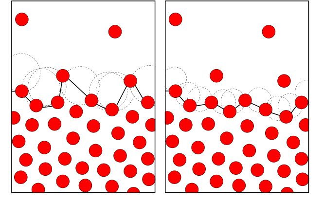
Figure 1: Schematic diagram of the $\alpha$-shape construction. For the sake of simplicity, a two-dimensional construction is shown. Left: a set of particles (red circles) is endowed with an $\alpha$-shape (whose border is plotted with a solid line) corresponding to “scoops” of radius $R$; dashed circles represent scoops with maximum penetration (touching two particles). Right: for the same particles, a smaller scoop radius produces a different $\alpha$-shape.

Two limits will perhaps clarify the procedure. If $\alpha$ is very small, all of the points will be reached; the resulting shape is, therefore, all of the $N$ points — but none of them will belong to the “border”. The other limit is perhaps more interesting: for values of $\alpha$ very large, the scoop takes half-spaces out, and can only reach the points that protrude from the surface. In this limit, the resulting $\alpha$-shape has as its border the very well-known convex hull of a set of points. We have made use of the Computational Geometry Algorithms Library (Cgal) [24], which provides highly efficient codes for these kind of structures. The $\alpha$-shape is evaluated in this library at little additional computational cost once a Delaunay triangulation is computed: the empty sphere condition permits to associate a given radius to each tetrahedron, below which the scoop will be able to “get in”. It is therefore a matter of bookkeeping to find the accessible points given some $\alpha$ value. More technically, the $\alpha$-shape is build in the (default) regularized mode, which eliminates isolated faces, and the border points are identified as the “regular” points [25].

This procedure is related to a recent proposal by L.B. Pàrtay and collaborators [26], in which they employ spheres approaching the surface in the normal direction, from the vapor side. This method and the one examined here are likely to provide similar results at low temperatures. At higher ones, on the other hand, their method will be hampered by molecules that are either in the vapor phase or loosely attached to the surface. Moreover, it will miss overhangs, whose role may be important at temperatures close to the critical point (note that this also applies to the MA methods, since they assume a surface defined mathematically by a single function $z=\xi(x,y)$, which cannot present overhangs.) In this sense, the current method can be considered more robust and reliable; moreover, it can be computationally more efficient than either the methods of Ref. [26] or MA methods (we will discuss efficiency in the next section). In addition, this method is not restricted to flat interfaces and can readily be applied to other interfaces, such as curved ones. This may be very useful in studies of nucleation (or cavitation), where a knowledge of the interfacial properties of droplets (or bubbles) may be desirable — this method may also be employed for micelles and other supramolecular aggregates. In fact, for most results we do not need to distinguish between an “upper” and “lower” interface, since the method selects both of them automatically. It is also easy to label each of the particles in the system as being part of the IS, next to it, second next to it, etc, since the Delaunay tessellation provides a well defined definition of neighborhood (as explored in the context of correlation functions in Ref. [19]).

Another relevant reference is the work by J. Chowdhary and B.M. Ladanyi [27]. In their work, the selection of surface molecules is alleviated because they consider binary interfaces between water and hydrocarbons. Since the two components are nearly immiscible, a simple definition of proximity to the opposing species can be employed to identify pivots. They go forward and construct an IS, a step not taken in Pàrtay et al [26]. In a spirit similar to this article, concepts of computational geometry are employed: the pivots are projected onto the plane of the interface, and a Voronoi tessellation is constructed (this procedure is closely related to the one termed “Delaunay Terrain” in the Cgal) documentation [24].) This allows an association of each non-surface molecule with a surface one, from which intrinsic profiles may be computed. In line with the MA results, structured intrinsic profiles are found for water, even when average profiles are monotonous (for hydrocarbons both are structured, the intrinsic ones more so.)

The method as implemented in Cgal is suitable only for “open” boundary conditions. E.g., an additional “point at infinity” is introduced when computing triangulations. Our system features periodic boundary conditions, which are not yet implemented in Cgal (a project to include them is underway [28]). We therefore choose the clumsy, but effective, procedure of replicating slabs of our cell, then neglecting the points which are outside the original cell. We have made sure these slabs are wide enough, $4\sigma$, for the boundary conditions to be well represented.

2 Methodology

We simulate a fluid with $2592$ particles interacting through a Lennard-Jones (LJ) potential:

$$u(r)=\epsilon\left\{\left(\frac{\sigma}{r}\right)^{12}-\left(\frac{\sigma}{r}\right)^{6}-\left(\frac{\sigma}{r_{\mathrm{c}}}\right)^{12}+\left(\frac{\sigma}{r_{\mathrm{c}}}\right)^{6}\right\}.$$ (3)

Interactions are truncated at a cutoff radius of $r_{\mathrm{c}}=3.02\sigma$. Particles are confined in a rectangular cell of dimensions $L_{x}=L_{y}=L=10.46\sigma$ and $L_{z}=90\sigma$; periodic boundary conditions are applied in all directions. Standard molecular dynamics simulations are carried out, with a time-step $dt=4.56\times 10^{-3}\sigma\sqrt{m/\epsilon}$ (in reduced units), using the software package dl_poly [29]. After an equilibration period of $10^{6}$ steps, particles form a liquid slab in the $x$-$y$ plane, surrounded by vapor. The temperature is set at $k_{B}T=0.678\epsilon$ by a Nose-Hoover thermostat. This has been found to be the triple point temperature for this truncated LJ potential, and hence the lowest temperature at which the liquid is thermodynamically stable. A production run of $50000$ steps is carried out, in the microcanonical ensemble, in order to avoid possible artifacts of the thermostat on the dynamics (which will be important for one of the methods explained below). Interfacial dynamics is slow enough to let us analyze $1$ configuration out of $10$, so we have to sample $5000$ configurations.

This choice of parameters (specially, number of particles and cutoff radius) leads to a very fast computation, that may be carried out even in a standard modern laptop computer. The reason for carrying out this simple simulation is that we will compare our results with MA. The later technique is quite heavy computationally, so that its configurational analysis ends up being more time-consuming than the simulation itself. For this number of particles, the MA analysis takes a CPU time about $10$ times longer than the simulation. The current procedure takes a time comparable to the simulation, depending on the information requested (about the same for the number of pivots, twice as much to build the intrinsic profile, $10$ times as much for the Fourier analysis described below.) Moreover, the MA procedure grows with the number of particles as $N^{2}$ (if the surface area is scaled suitably, so that the area grows as a power $2/3$ of the number of particles), whereas the current procedure grows as bad only in the worst case: typically, it grows only as $N\log(N)$ [the Fourier analysis scales as $N^{2/3}\log(N)$ .] We have carried out additional runs in order to get error bar estimations for some calculations, as will be indicated.

In order to define the border between the liquid and vapor phases, $\alpha$-shapes are employed. The particles that define this border, which will be the outmost liquid layer, will be called “pivots”, keeping the standard nomenclature. The idea is to obtain these pivots as the points belonging to an $\alpha$-shape. Notice that the resulting shape is not a smooth surface, as in previous approaches, but a triangulated one.

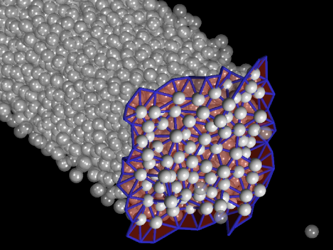
Figure 2: (Color online) Snapshot of one of our configurations. Molecules are pictured as white balls, translucent unless they belong to the intrinsic surface, in which case they are solid. The $\alpha$-shape border, for $\alpha=R^{2}$, $R=1.2$, is the red triangulation, with edges in blue.

A first issue arises from the fact that there are isolated particles that belong to the gas that will be included as part of this shape for any reasonable value of $\alpha$. This is easily taken care of by choosing the points that have surface neighbors in the sense given above (having a sphere of radius $R$ touching all three), and marking the rest as isolated. In the Cgal implementation, this is taken care of by choosing the regular points in the regularized mode, as commented above. This procedure, indeed, is similar to the percolation analysis that is employed as a first step in MA approaches. In Fig. 2 we show a snapshot of our configuration and the resulting $\alpha$-shape, for a typical choice of $\alpha$ explained below.

3 Results

Of course, the main task is to determine the optimal value of the scoop radius, $R$, or equivalently the right $\alpha$-shape (since $\alpha=R^{2}$.)

At variance with many previous applications, the system under consideration has some well defined length scales. For dense phases, such as the liquid, the interparticle spacing is always close to the distance at which the potential has its minimum ($2^{1/6}\sigma$ for the LJ fluid). Some of the particles may be slightly further, but they can never be much closer, since at some distance hard-core repulsion sets in (around $\sigma$ for the LJ fluid). This means that a choice of $R<\sigma$ will result in the selection of all of the particles as belonging to the $\alpha$-shape, a nonsensical result from a physical point of view. Values of $R$ too high, on the other hand, result in few pivots being selected, and a nearly flat shape (with our boundary conditions, one outmost molecule at each interface will be selected as a pivot, with horizontal interfaces.) In practice, we will need to consider a range $\sigma<R<2\sigma$, or $\sigma^{2}<\alpha<4\sigma^{2}$.

There are several ways to determine this value, which should yield the same result (within error intervals):

• examination of the profiles,

• pivot dynamics, and

• comparison against previous, reliable, results.

These three paths are described in the next subsections.

3.1 Structure

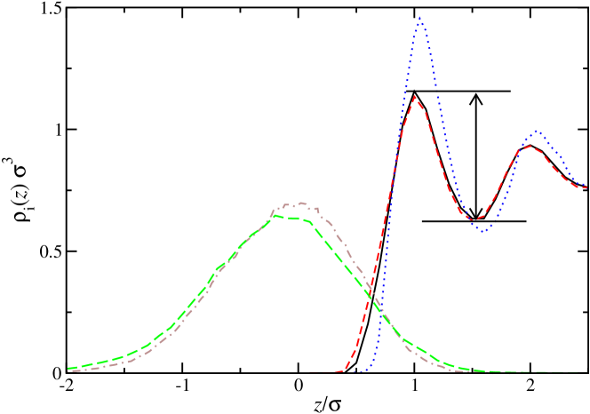
Figure 3: Density profiles as functions of the coordinate across the interface. Solid black line: intrinsic density profile $\rho_{i}(z)$ obtained by the current method, for $R=1.20\sigma$; dashed red line: $\rho_{i}(z)$ obtained by the current method, for $R=1.30\sigma$; blue dotted line: MA $\rho_{i}(z)$ taken from Ref. [30]. The vertical arrow marks the difference that serves as a measure of order. Green long-dashed line: pivot profile $\rho_{s}(z)$ obtained by the current method, for $R=1.30\sigma$; brown dot-dashed line: MA $\rho_{s}(z)$ taken from Ref [13]. The two later curves are normalized to unity.

The first route is through careful examination of details of the profiles. Several profiles can be obtained: the average profile, $\rho(z)$, the pivot profile $\rho_{s}(z)$, and the intrinsic profile $\rho_{i}(z)$. The first is of course independent of the procedure to obtain the IS. The overall shape and decay of the other two are features that have been used in order to determine the best value of the parameters. As discussed in Refs. [30, 31], this is quite painstaking and fine-tuning is difficult. For example, in Fig. 3 we plot results for $R=1.20\sigma$ and $R=1.30\sigma$ which, as we will see, are close to optimal; it is clearly difficult to judge which profile is “best.” We therefore focus on a specific detail of the profiles: the difference between the height of the first peak and the next trough (the one between the first and second peaks). This distance will be a measure of the structure of the intrinsic profile.

In principle, a more structured profile should be preferable. The argument behind this claim is partly circular: given that we assume the existence of some IS which provides some intrinsic density profile (much rougher than the average one), the best criterion is the one that results in the rougher profiles (always, of course, within some logical physical limits) [32]. In fact, this criterion enables us to compare different methods, as we will see in §3.3. Of course, this point of view should not be pushed too far, and profiles that oscillate unphysically, or present other unlikely features, should be discarded. Ultimately, a comparison with results obtained by other methods (such as experiments) would favor one method or another, but for the time being this comparison is not possible.

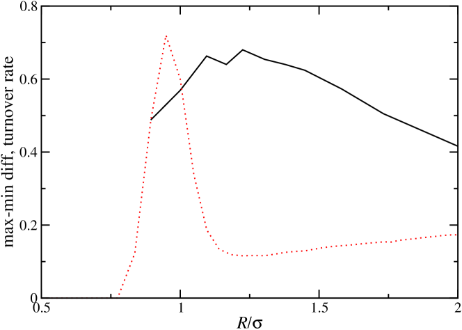
Figure 4: (Color online) Solid black line: difference between heights of the first peak and next trough of the intrinsic profile (see arrow in Fig. 3 for a particular case), versus scoop radius $R$. Dotted red line: Pivot turnover rate (arbitrary units) versus scoop radius $R$.

In Fig. 3 we draw vertical segments that represents the measure of structure. for two particular choices; the collected values are plotted in Figure 4. Apart from some noise, an optimal value of $R$ of about $1.2\sigma$ is clearly identified — this could be anticipated, as it is close to the mean interparticle distance in the bulk liquid, which in turn is similar to the value at which the LJ potential has its minimum.

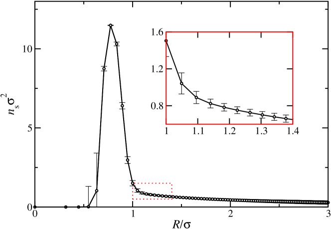
Figure 5: (Color online) Surface density (pivots per unit area) versus scoop radius $R$. The error bars correspond to the variance of the density due to different samples. Inset: blow-up of relevant region, shown as a red dotted box in the main graph.

In Fig. 5 we show the calculated surface density $n_{s}$, an important surface characteristic which is simply defined by the number of pivots per unit projected area (i.e., the nominal area, not the area of the IS). The inset shows a blow-up of the area most relevant for this study. For $R=1.2\sigma$ we can read off the value $n_{s}=(0.77\pm 0.2)\sigma^{-2}$, to be compared with previous estimate [31] of $0.80\sigma^{-2}$.

3.2 Dynamics

As shown recently [31], dynamics can provide a reliable, independent way of obtaining the optimal parameters for the IS, apart from the obvious interest in dynamical features of the interface [13]. A key quantity in this regard is the turnover rate: the number of molecules per unit area and per unit time that enter the IS (i.e., that become pivots). This number also equals the number of molecules that leave the IS, on average (or, exactly if the number is fixed, as in most recent MA approaches [30, 33, 34].) The pivot residence time is physically influenced by the fluid dynamics at the molecular level, but it is also tied to the specific choice of IS. If the number of pivots is too high, there will be a high number of them that enter and leave the IS at each time-step: many of these pivots should not be included in a physical IS, and this high turnover is spurious. If, on the other hand, the number of pivots is too low, the IS will change its shape a great deal, jumping from a set of pivots to another one, thus causing a high turnover. The best parameter is, in principle, the one for which a minimum in turnover rate is found. This argument applies most directly to procedures in which the number of pivots is fixed, but it may be applied to other parameters, such as $R$, that indirectly affect this number (with a clear dependency, as shown in Fig. 5). In Fig. 4 we plot this turnover rate, which identifies a value of $R=1.23\sigma$ — this is in rather good agreement with the previous value of $1.2\sigma$. The corresponding surface density is $n_{s}=(0.74\pm 0.2)\sigma^{-2}$.

A related criterion, not strictly dynamical in nature, is to check the variance implied in the error bars of Fig. 5. This quantity shows a minimum at $R=1.25\sigma$, in very good agreement with the previous value (there is a deeper minimum at $R\approx 0.75\sigma$, but this range is unphysical).

3.3 Comparison to known results

We may compare the resulting intrinsic density profiles with the ones from the MA method. In Fig. 3 we also show (bell-shaped curves) the density profile of surface molecules (pivots), $\rho_{s}(z)$, compared with a previous MA profile. The parameter $R$ is set to $1.3\sigma$, which, as has been explained, is close to optimal. Our current results show a slight decrease of central pivots and an increase of peripheral ones. This means the $\alpha$-shape is including molecules slightly toward the two bulk phases, which are not part of the MA list, and neglecting some interfacial ones. This does not seem desirable, but the two curves are seen to be quite close in shape.

On the other hand, a comparison of our intrinsic density profile $\rho_{i}(z)$, already discussed, with the MA one (both included in the same Figure, with a solid and dotted lines) clearly shows that the current method, despite its elegance, still performs worse than the MA one. Keeping the criterion employed in §3.1, a stronger structure signals a better method, and our intrinsic profiles, while showing distinct layering, are smoother than the MA ones. We will discuss possible improvements in the Conclusions section, but for now let us take this as an indication that MA results may be taken as close to the “optimal” ones.

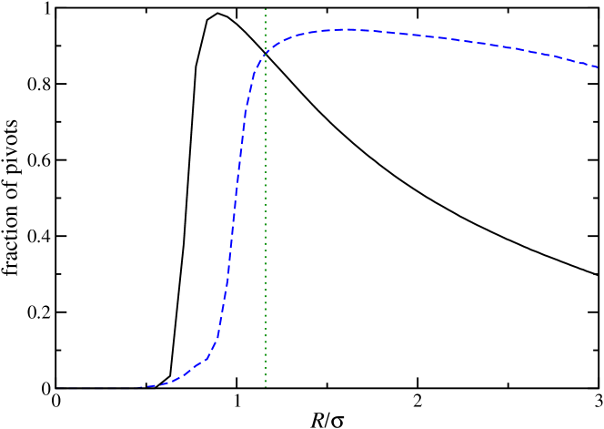
Figure 6: (Color online) Fraction of pivots versus scoop radius $R$. Solid black line: fraction of MA pivots that are part of our pivots. Dashed blue line: fraction of our pivots that are part of MA pivots. The dotted green vertical line provides the intersection of the curves, at $R=1.16\sigma$.

We may now use this idea in order to rapidly establish the optimal values of $R$, by comparing against the MA results. In Fig. 6 we plot (solid line) the fraction of MA pivots that are part of our pivots.The agreement is fairly low for high values of $R$, since very few pivots are selected in this case (recall only the most exposed molecules are selected for very high values of $R$). The agreement then increases, and goes to almost $1$ at values around $\sigma$. This means all MA pivots are included in our set, but this is hardly surprising, since around this range most molecules are selected as borders of the $\alpha$-shape, including of course most MA pivots (see the high peak in Fig. 5). The information can therefore be completed by considering the fraction of our pivots that are contained in the MA list. This curve is also plotted in Fig. 6 with a dashed line. The behavior is qualitatively similar, but this time the maximum is much more rounded, and occurs at higher values, around $1.5\sigma$. Since the maxima do not coincide, we may take the value at the intersection of the two curves as the best compromise. At this value, about $88$% of the MA pivots are included in our list, and $88$% of our pivots are included in the MA list. This value turns out to be $R=1.16\sigma$, again in good agreement with previous estimates. Alternatively, this crossing is the point for which both methods coincide in the value of the surface density, $n_{s}=0.80\sigma^{-2}$. (If a set A contains a fraction of elements common with another set B, and B contains the same fraction of elements common with A, both sets must have the same size.) An alternative procedure would therefore be to select the value of $R$ for which a previously known surface density is recovered.

Figure 7: Fraction of MA pivots that are part of our pivots versus anisotropy parameter $D$.

Given the strong anisotropy of the interface in the direction across it, we have also explored the possibility that one may obtain better results with the use of ellipsoidal scoops, instead of spherical ones. (The same numerical libraries may be used, since what we effectively do is to compress the system in the $z$ direction instead, while keeping the scoops spherical.) The scoops would be defined by

$$(x/R)^{2}+(y/R)^{2}+(z/DR)^{2}=1,$$

with two parameters, $R$ as before, and $D$ measuring the anisotropy. This new parameter, $D$, is explored in Fig. 7. For each value of $D$ the optimum value of $R$ is found, and the curves therefore implies different values of the later, which is $1.16$ at $D=1$. It is apparent that the best value turns out to be very close to $D=1$. This is also the case for the methods above (result not shown): the difference in height is maximal for this value, the minimum of the turnover rate is shallower for other values of $D$, and does not coincide with the minimum of the variance. Hence, the idea of using ellipsoidal scoops can be rejected, at least for this simple liquid.

Since our triangulated mesh is a perfectly defined mathematical entity, a full Fourier transform of the surface can be carried out, at an arbitrary level of detail. This is at variance with the MA procedure, in which a higher cutoff wave-vector $q_{u}$ must be introduced in order the method be mathematically tractable. While there is a physical reason for this wave-vector being close $q_{u}=2\pi/\sigma$ (as usually done in CWT, see Eq. 2), finding its precise value has been delicate.

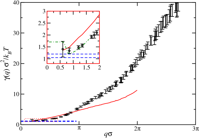
Figure 8: (Color online) Wavenumber-dependent surface tension $\gamma(q)$ in reduced units. Black bars: current results, with error bars; solid red line: MA results [35] for $n_{s}=0.8\sigma^{-2}$, $q_{u}=2\pi/\sigma$; dashed blue line: range of values for the bulk surface tension, obtained by the method of [36]. The inset shows a blow-up of the low-$q$ region, shown as a red dotted box in the main graph. In it, a possible deepest-minimum situation is plotted with a green dot-dashed line.

In Fig. 8 we compare results from the Fourier analysis of our IS surface with recent MA results. In particular, we compute the very important surface tension spectrum; CWT establishes the mean square fluctuations of Fourier mode given in Eq. 1 above. This expression is seen to be only valid at low $q$ values; at higher values, the $q$ dependence is taken care of by defining a $q$-dependent surface tension:

$$\gamma(q)\equiv\frac{k_{B}T}{Aq^{2}\left\langle\left|\xi_{q}\right|^{2}\right\rangle}.$$

The main argument behind CWT hinges on this function increasing with $q$, otherwise the surface would be unstable against high-$q$ perturbations. In order to refine our precision, we have carried out $4$ additional runs, and used results from the two interfaces present in the system, in order to obtain $8$ values for each value of $q$. We have used their mean value as our measured quantity, and their standard deviation as its error bar. The error bars are seen to be increasingly smaller at lower values of the wave-vector, with statistical errors increasing at higher values

In the same graph we include previous MA results for this system [35], and the bulk surface tension. For the later quantity, a new simulation has been carried out at this particular temperature and potential cutoff; we indicate the range of the surface tension, that is, a band centered in the mean value and with a width given by the error, calculated as in Ref. [36]. Our curve is qualitatively similar to the MA one: both tend to the bulk value in the limit $q\rightarrow 0$ and then increase, and both increase further for high values of the wave-vector, in accordance with the CWT thesis. Quantitatively, they differ in the values of $\gamma(q)$, with the MA curve starting out with a higher slope, but then growing slower than our curve at higher values of $q$.

At this point, we must mention that our results share a feature with those from MA: the absence of an intermediate minimum between the limits of very small and very large wave-vectors. To be more precise, our error bars would in principle allow for a minimum around $q=1/\sigma$, as shown in the Figure’s inset, where a possible deepest-minimum situation is depicted. However, the inset also shows that this minimum is not likely to be present at all, given the range of the values for the bulk surface tension.

The presence of a minimum would imply the enhanced amplitude of capillary waves with wave-vectors around it. This possibility has been predicted theoretically by Mecke and Dietrich [37], improving previous efforts [38]. The theory was later expanded [39, 40, 41, 42] and received support from simulations [43]. Remarkably, experimental work has also confirmed this prediction [44, 45, 46, 47, 48]. However, other experimental teams have pointed out technical difficulties in the interpretation of the experimental data [49, 50]. Likewise, the main theoretical framework has been recently challenged [51]. There are indications (see recent Ref. [52]) that this disagreement stems from whether the IS is defined from the molecular positions (as in this work), or from molecular distributions (such as a set of Gibbs dividing surfaces).

4 Conclusions

We have presented an application of the $\alpha$-shape concept, taken from the field of computational geometry, to the identification of the intrinsic surface of a liquid-vapor interface. Compared with the minimum area method, the method may have a lower performance, as indicated by the less structured intrinsic density profiles. However, the method is elegant and computationally very simple. Both from a computational point of view and, more importantly, from a mathematical one. The resulting IS is a triangulated mesh, which is a perfectly defined mathematical entity. As a result, a full Fourier transform of the surface can be carried out, at an arbitrary level of detail. Our results for the surface tension spectrum are qualitatively similar to the ones from MA, even in quantitatively different. In particular, no sizable minimum in the surface tension is observed.

We therefore feel that the current method shows a number of interesting features. Even if still inferior to the MA method, further developments could refine it and make it comparable. It is interesting, in this regard, to incorporate some of the basic ideas of MA in the procedure: either minimum-area requirements, or incremental adding of pivots to an existing surface.

5 Acknowledgments

Financial support for this work has been provided by the Dirección General de Investigación, Ministerio de Ciencia y Tecnología of Spain, under grants FIS2004-05035-C03, FIS2007-65869-C03, and CTQ2005-00296/PPQ and Comunidad Autónoma de Madrid under program MOSSNOHO-CM (S-0505/Esp-0299).

References

- [1] D Frenkel and B Smit. Understanding Molecular Simulation. Academic Press, second edition, 2002.
- [2] J S Rowlinson and Benjamin Widom. Molecular Theory of Capillarity. Dover, 2002.
- [3] O. M. Magnussen, B. M. Ocko, M. J. Regan, K. Penanen, P. S. Pershan, and M. Deutsch. X-ray reflectivity measurements of surface layering in liquid mercury. Phys. Rev. Lett., 74(22):4444–4447, May 1995.
- [4] M. J. Regan, E. H. Kawamoto, S. Lee, P. S. Pershan, N. Maskil, M. Deutsch, O. M. Magnussen, B. M. Ocko, and L. E. Berman. Surface layering in liquid gallium: An x-ray reflectivity study. Phys. Rev. Lett., 75(13):2498–2501, Sep 1995.
- [5] E. DiMasi, H. Tostmann, B. M. Ocko, P. S. Pershan, and M. Deutsch. X-ray reflectivity study of temperature-dependent surface layering in liquid hg. Phys. Rev. B, 58(20):R13419–R13422, Nov 1998.
- [6] H. Tostmann, E. DiMasi, B. M. Ocko, M. Deutsch, and P. S. Pershan. X-ray studies of liquid metal surfaces. Journal of Non-Crystalline Solids, 250-252(Part 1):182 – 190, 1999.
- [7] E Chacón, M Reinaldo-Falagán, E Velasco, and P Tarazona. Layering at free liquid surfaces. Phys. Rev. Lett., 87(16):166101, Sep 2001.
- [8] E Velasco, P Tarazona, M Reinaldo-Falagán, and E Chacón. Low melting temperature and liquid surface layering for pair potential models. J. Chem. Phys., 117(23):10777–10788, 2002.
- [9] Scott W. Sides, Gary S. Grest, and Martin-D. Lacasse. Capillary waves at liquid-vapor interfaces: A molecular dynamics simulation. Phys. Rev. E, 60(6):6708–6713, Dec 1999.
- [10] Ahmed E Ismail, Gary S Grest, and Mark J Stevens. Capillary waves at the liquid-vapor interface and the surface tension of water. J. Chem. Phys., 125(1):014702, 2006.
- [11] E Chacón and P Tarazona. Intrinsic profiles beyond the capillary wave theory: A monte carlo study. Phys. Rev. Lett., 91(16):166103, Oct 2003.
- [12] P Tarazona and E Chacón. Monte carlo intrinsic surfaces and density profiles for liquid surfaces. Phys. Rev. B, 70(23):235407, 2004.
- [13] Daniel Duque, Enrique Chacón, and P Tarazona. Diffusion at the liquid-vapor interface. J. Chem. Phys., 128(13):134704, 2008.
- [14] H Edelsbrunner, D G Kirkpatrick, and R Seidel. On the shape of a set of points in the plane. IEEE Trans. Inform. Theory, 29(4):551–559, 1983.
- [15] H Edelsbrunner and E P Mücke. Three-dimensional alpha shapes. ACM Trans. Graph., 13(1):43–72, 1994.
- [16] Atsuyuki Okabe, Barry Boots, Kokichi Sugihara, and Sung Nok Chiu. Spatial tessellations. Concepts and applications of Voronoi diagrams. John Wiley & Sons, 2000.
- [17] N N Medvedev, A Geiger, and W Brostow. Distinguishing liquids from amorphous solids: Percolation analysis on the voronoi network. J. Chem. Phys., 93(11):8337–8342, 1990.
- [18] J C Gil Montoro and J L F Abascal. The Voronoi polyhedra as tools for structure determination in simple disordered systems. J. Phys. Chem., 97:4211–4215, 1993.
- [19] V S Kumar and V Kumaran. Voronoi neighbor statistics of hard-disks and hard-spheres. J. Chem. Phys., 123(7):074502, 2005.
- [20] V S Kumar and V Kumaran. Voronoi cell volume distribution and configurational entropy of hard-spheres. J. Chem. Phys., 123(11):114501, 2005.
- [21] Jared T Fern, David J Keffer, and William V Steele. Measuring coexisting densities from a two-phase molecular dynamics simulation by voronoi tessellations. J. Phys. Chem. B, 111(13):3469–3475, 2007.
- [22] Jared T Fern, David J Keffer, and William V Steele. Vapor-liquid equilibrium of ethanol by molecular dynamics simulation and voronoi tessellation. J. Phys. Chem. B, 111(46):13278–13286, 2007.
- [23] Biogeometry Project, Duke University. http://biogeometry.cs.duke.edu.
- [24] Cgal, Computational Geometry Algorithms Library. http://www.cgal.org.
- [25] Tran Kai Frank Da and Mariette Yvinec. 3d alpha shapes. In CGAL Editorial Board, editor, CGAL User and Reference Manual. 3.3 edition, 2007.
- [26] L B Pártay, G Hantal, P Jedlovsky, A Vincze, and G Horvai. A new method for determining the interfacial molecules and characterizing the surface roughness in computer simulations. application to the liquid-vapor interface of water. J. Comput. Chem., 29(6):945–956, 2008.
- [27] J Chowdhary and B M Ladanyi. J. Phys. Chem. B, 110:15442, 2006.
- [28] Monique Teillaud. Private communication.
- [29] W Smith. Mol. Sim., 32:933–1121, 2006.
- [30] Enrique Chacón and Pedro Tarazona. Characterization of the intrinsic density profiles for liquid surfaces. J. Phys.: Cond. Matter, 17(45):S3493–S3498, 2005.
- [31] E Chacón, D Duque, and P Tarazona. to be published.
- [32] Pedro Tarazona. Private communication.
- [33] E Chacón, P Tarazona, and L E González. Intrinsic structure of the free liquid surface of an alkali metal. Phys. Rev. B, 74(22):224201, 2006.
- [34] Enrique Chacón, Pedro Tarazona, and José Alejandre. The intrinsic structure of the water surface. J. Chem. Phys., 125(1):014709, 2006.
- [35] Enrique Chacón. Data kindly provided by this author.
- [36] Daniel Duque, Josep C Pàmies, and Lourdes F Vega. Interfacial properties of lennard-jones chains by direct simulation and density gradient theory. J. Chem. Phys., 121:11395—11403, 2004.
- [37] K R Mecke and S Dietrich. Phys. Rev. E, 59:6766, 1999.
- [38] M. Napiórkowski and S. Dietrich. Structure of the effective hamiltonian for liquid-vapor interfaces. Phys. Rev. E, 47(3):1836–1849, Mar 1993.
- [39] Ronald Lovett and Marc Baus. Thermodynamic forces in highly curved fluid interfaces. The Journal of Chemical Physics, 120(22):10711–10727, 2004.
- [40] T Hiester, S Dietrich, and K R Mecke. J. Chem. Phys., 125:184701, 2006.
- [41] J. Stecki. Phys. Rev. B, 74:033409, 2006.
- [42] José G. Segovia-López and Víctor Romero-Rochín. Interfacial properties of liquid-vapor interfaces with planar, spherical, and cylindrical geometries in mean field. Physical Review E (Statistical, Nonlinear, and Soft Matter Physics), 73(2):021601, 2006.
- [43] R. L. C. Vink, J. Horbach, and K. Binder. Capillary waves in a colloid-polymer interface. The Journal of Chemical Physics, 122(13):134905, 2005.
- [44] C Fradin, A Braslau, D Luzet, D Smilgies, M Alba, N Boudet, K Mecke, and J Daillant. Nature, 403:871–874, 2000.
- [45] S. Mora, J. Daillant, K. Mecke, D. Luzet, A. Braslau, M. Alba, and B. Struth. X-ray synchrotron study of liquid-vapor interfaces at short length scales: Effect of long-range forces and bending energies. Phys. Rev. Lett., 90(21):216101, May 2003.
- [46] Dongxu Li, Bin Yang, Binhua Lin, Mati Meron, Jeff Gebhardt, Tim Graber, and Stuart A. Rice. Wavelength dependence of liquid-vapor interfacial tension of ga. Phys. Rev. Lett., 92(13):136102, Apr 2004.
- [47] Binhua Lin, Mati Meron, Jeff Gebhardt, Tim Graber, Dongxu Li, Bin Yang, and Stuart A. Rice. X-ray diffuse scattering study of height fluctuations at the liquid-vapor interface of gallium. Physica B: Condensed Matter, 357(1-2):106 – 109, 2005. Proceedings of the 8th International Conference on Surface X-ray and Neutron Scattering.
- [48] Dongxu Li, Xu Jiang, Binhua Lin, Mati Meron, and Stuart A. Rice. Diffuse scattering from the liquid-vapor interfaces of dilute , , and alloys. Phys. Rev. B, 72(23):235426, Dec 2005.
- [49] P. S. Pershan. Effects of thermal roughness on x-ray studies of liquid surfaces. Colloids and Surfaces A: Physicochemical and Engineering Aspects, 171(1-3):149 – 157, 2000.
- [50] Oleg Shpyrko, Masafumi Fukuto, Peter Pershan, Ben Ocko, Ivan Kuzmenko, Thomas Gog, and Moshe Deutsch. Surface layering of liquids: The role of surface tension. Phys. Rev. B, 69(24):245423, Jun 2004.
- [51] P Tarazona, Ramiro Checa, and Enrique Chacón. Critical analysis of the dft prediction of enhanced cws. Phys. Rev. Lett., 99:196101, 2007.
- [52] Edgar M. Blokhuis. On the spectrum of fluctuations of a liquid surface: From the molecular scale to the macroscopic scale. The Journal of Chemical Physics, 130(1):014706, 2009.