Haar Wavelets-Based Approach for Quantifying Credit Portfolio Losses

Abstract

This paper proposes a new methodology to compute Value at Risk (VaR) for quantifying losses in credit portfolios. We approximate the cumulative distribution of the loss function by a finite combination of Haar wavelets basis functions and calculate the coefficients of the approximation by inverting its Laplace transform. In fact, we demonstrate that only a few coefficients of the approximation are needed, so VaR can be reached quickly. To test the methodology we consider the Vasicek one-factor portfolio credit loss model as our model framework. The Haar wavelets method is fast, accurate and robust to deal with small or concentrated portfolios, when the hypothesis of the Basel II formulas are violated.

1 Introduction

It is very important for a bank to manage the risks originated from its business activities. In particular, the credit risk underlying the credit portfolio is often the largest risk in a bank. The measured credit risk is then used to assign capital to absorb potential losses arising from its credit portfolio.

The Vasicek model is the basis of the Basel II IRB approach. It is a Gaussian one factor model such that default events are driven by a latent common factor that is assumed to follow a Gaussian distribution, also called Asymptotic Single Risk Factor (ASRF) model. Under this model, loss only occurs when an obligor default in a fixed time horizon. If we assume certain homogeneity conditions, this one factor model leads to a simple analytic asymptotic approximation for the loss distribution and Value at Risk (VaR). This approximation works well for a large number of small exposures but can underestimate risks in the presence of exposure concentrations.

Concentration risks in credit portfolios arise from an unequal distribution of loans to single borrowers (name concentration) or different industry or regional sectors (sector or country concentration). Moreover, certain dependencies as, for example, direct business links between different borrowers, can increase the credit risk in a portfolio since the default of one borrower can cause the default of a dependent second borrower. This effect is called default contagion and is linked to both name and sector concentration.

In credit risk management one is particularly interested in the portfolio loss distribution. Since the portfolio loss is usually modeled as a sum of random variables, the main task is to evaluate the probability density function (PDF) of such a sum. The PDF of a sum of random variables is equal to the convolution of the respective PDFs of the individual asset loss distributions. The evaluation of this convolution is a difficult problem analytically, is computationally very intensive and in full generality is impractical for any realistically sized portfolio.

For all these reasons, several methods have been developed in the last years. The saddle point approximation due to [Mar01a] gives an analytical approximation of the Laplace inversion of the moment generating function (MGF). This method has been improved by [Mar06] based on conditional independence models. [Gla07] applies the methodology developed by [Aba00] to the single-factor Merton model. First, the Bromwich integral is approximated by an infinite series using the trapezoidal rule and second, the convergence of the infinite series is accelerated by a method called Euler summation. They have shown that the cumulative distribution function (CDF) is comparatively accurate in small loss region, whereas the accuracy worsens in the tail region. This is because the infinite series obtained by the Euler summation is an alternating series, each term of which has a very large absolute value.

Another approach to numerically invert the Laplace transform has been studied by [Hoo82] and [Ahn03] consisting in applying the Poisson algorithm to approximate the Bromwich integral by an infinite series, as in [Aba00] and then use the quotient-difference (QD) algorithm to accelerate the slow convergence of the infinite series. We will refer to this approach as the Hoog algorithm. [Tak08] has applied this methodology to the multi-factor Merton model. The numerical examples presented show that in contrast with the Euler summation technique, de Hoog algorithm is quite efficient in measuring tail probabilities.

In this paper, we present a novel methodology for computing VaR through numerically inverting the Laplace Transform of the CDF of the loss function once we have approximated it by a finite sum of Haar wavelets basis functions. This kind of functions have compact support and so make them useful to study local properties of the approximated function. Moreover, the CDF of the loss function is discontinuous, making more suitable this way of approximation.

The remaining parts of the paper are organized as follows. In the next section we present the one-factor Gaussian copula model and we define VaR as the risk measure used to quantify losses in Basel II Accord. In section three we present the basic theory about Haar wavelets basis system used for the approximation detailed in section four. Finally, we show with numerical examples the speed and accuracy of the new method in section five and section six is devoted to conclusions.

2 Portfolio Loss and Value at Risk

To represent the uncertainty about future events, we specify a probability space $(\Omega,\mathcal{F},\mathbb{P})$ with sample space $\Omega$, $\sigma$-algebra $\mathcal{F}$, probability measure $\mathbb{P}$ and with filtration $(\mathcal{F}_{t})_{t\geq 0}$ satisfying the usual conditions. We fix a time horizon $T>0$. Usually $T$ equals one year.

Consider a credit portfolio consisting of $N$ obligors. Any obligor $n$ can be characterized by three parameters: the exposure at default $E_{n}$, the loss given default which without loss of generality we assume to be $100\%$ and the probability of default $P_{n}$, assuming that each of them can be estimated from empirical default data. The exposure at default of an obligor denotes the portion of the exposure to the obligor which is lost in case of default. Let $D_{n}$ be the default indicator of obligor $n$ taking the following values

$$D_{n}=\left\{\begin{array}[]{ll}1,&\textrm{if obligor $n$ is in default,}\\ 0,&\textrm{if obligor $n$ is not in default,}\end{array}\right.$$

Let $L$ be the portfolio loss given by:

$$L=\sum_{n=1}^{N}L_{n},$$

where $L_{n}=E_{n}\cdot D_{n}$.

To test our methodology we consider the Vasicek one-factor Gaussian copula model as our model framework. The Vasicek model is a one period default model, i.e., loss only occurs when an obligor defaults in a fixed time horizon. Based on Merton‘s firm-value model, to describe the obligor’s default and its correlation structure, we assign each obligor a random variable called firm-value. The firm-value of obligor $n$ is represented by a common, standard normally distributed factor $Y$ component and an idiosyncratic standard normal noise component $\epsilon_{n}$. The $Y$ factor is the state of the world or business cycle, usually called systematic factor.

$$V_{n}(T)=\sqrt{\rho_{n}}Y+\sqrt{1-\rho_{n}}\epsilon_{n},$$

where $Y$ and $\epsilon_{n}$, $\forall n\leq{N}$ are i.i.d. standard normally distributed.

In case that $\rho_{n}=\rho$ for all $n$, the parameter $\rho$ is called the common asset correlation. The important point is that conditional on the realization of the systematic factor $Y$, the firm’s values and the defaults are independent. From now on, we assume $\rho_{n}$ to be constant.

Let us explain in detail the meaning of systematic and idiosyncratic risk. The first one can be viewed as the macro-economic conditions and affect the credit-worthiness of all obligors simultaneously. The second one represent conditions inherent to each obligor and this is why they are assumed to be independent of each other.

In the Merton model, each obligor $n$ defaults if its firm-value falls below the threshold level $T_{n}$ defined by $T_{n}\equiv{\Phi^{-1}(P_{n})}$ where $\Phi(x)$ is the standard normal cumulative distribution function and $\Phi^{-1}(x)$ denotes its inverse function. The probability of obligor $n$’s default conditional on a realization of $Y=y$ is given by

$$p_{n}(y)\equiv{\mathbb{P}(V_{n}<T_{n}\mid Y=y)}=\Phi\left(\frac{T_{n}-\sqrt{\rho}y}{\sqrt{1-\rho}}\right).$$

Consequently, the conditional probability of default depends on the systematic factor, reflecting the fact that the business cycle affect the possibility of an obligor’s default.

Let $F$ be the cumulative distribution function of $L$. Without loss of generality, we can assume $\sum_{n=1}^{N}E_{n}=1$ and consider

$$F(x)=\left\{\begin{array}[]{ll}\overline{F}(x),&\textrm{if $0\leqslant x\leqslant 1$,}\\ 1,&\textrm{if $x>1$,}\end{array}\right.$$

for a certain $\overline{F}$ defined in $[0,1]$.

Let $\alpha\in(0,1)$ be a given confidence level, the $\alpha$-quantile of the loss distribution of $L$ in this context is called Value at Risk (VaR). Thus,

$$l_{\alpha}=inf\{l\in\mathbb{R}:\mathbb{P}(L\leq l)\geq\alpha\}=inf\{l\in\mathbb{R}:F(l)\geq\alpha\}.$$

Usually the $\alpha$ of interest is very close to 1. This is the measure chosen in the Basel II Accord for the computation of capital requirement, which means a bank that manages its risks with Basel II must to reserve capital by an amount of $l_{\alpha}$ to cover extreme losses.

3 The Haar Basis Wavelets System

Consider the space $L^{2}(\mathbb{R})=\{f:\int_{-\infty}^{+\infty}\left|f(x)\right|^{2}dx<\infty\}$. For simplicity, we can view this set as a set of functions $f(x)$ which get small in magnitude fast enough as $x$ goes to plus and minus infinity.

A general structure for wavelets in $L^{2}(\mathbb{R})$ is called a Multi-resolution Analysis (MRA). We start with a family of closed nested subspaces

$$...\subset V_{-2}\subset V_{-1}\subset V_{0}\subset V_{1}\subset V_{2}\subset...$$

in $L^{2}(\mathbb{R})$ where

$$\bigcap_{j\in\mathbb{Z}}{V_{j}}=\{0\},\hskip 28.45274pt\displaystyle\overline{\bigcup_{j\in\mathbb{Z}}{V_{j}}}=L^{2}(\mathbb{R}),$$

and

$$f(x)\in V_{j}\Longleftrightarrow f(2x)\in V_{j+1}.$$

If these conditions are met, then there exists a function $\phi\in V_{0}$ such that $\{\phi_{j,k}\}_{k\in\mathbb{Z}}$ is an orthonormal basis of $V_{j}$, where

$$\phi_{j,k}(x)=2^{j/2}\phi(2^{j}x-k).$$

In other words, the function $\phi$, called the father function, will generate an orthonormal basis for each $V_{j}$ subspace.

Then we define $W_{j}$ such that $V_{j+1}=V_{j}\oplus W_{j}$. This says that $W_{j}$ is the space of functions in $V_{j+1}$ but not in $V_{j}$, and so, $L^{2}(\mathbb{R})=\sum_{j}\oplus W_{j}$. Then (see [Dau92]) there exists a function $\psi\in W_{0}$ such that $\{\psi_{j,k}\}_{k\in\mathbb{Z}}$ is an orthonormal basis of $W_{j}$, and $\{\psi_{j,k}\}_{j,k\in\mathbb{Z}}$ is a wavelets basis of $L^{2}(\mathbb{R})$, where

$$\psi_{j,k}(x)=2^{j/2}\psi(2^{j}x-k).$$

The function $\psi$ is called the mother function, and the $\psi_{j,k}$ are the wavelets functions.

For any function $f\in L^{2}(\mathbb{R})$ a projection map of $L^{2}(\mathbb{R})$ onto $V_{m}$,

$$\mathcal{P}_{m}:L^{2}(\mathbb{R})\rightarrow V_{m},$$

is defined by

$$\mathcal{P}_{m}f(x)=\sum_{j=-\infty}^{m-1}\sum_{k=-\infty}^{k=+\infty}d_{j,k}\psi_{j,k}(x)\\ =\sum_{k\in\mathbb{Z}}c_{m,k}\phi_{m,k}(x).$$ (1)

where $d_{j,k}=\int_{-\infty}^{+\infty}f(x)\psi_{j,k}(x)dx$ are the wavelets coefficients and the $c_{m,k}=\int_{-\infty}^{+\infty}f(x)\phi_{m,k}(x)dx$ are the scaling coefficients. The first part in (1) is a truncated wavelets series. If $j$ were allowed to go to infinity, we would have the full wavelets summation. The second part in (1) gives an equivalent sum in terms of the scaling functions $\phi_{m,k}$. Considering higher $m$ values, meaning that more terms are used, the truncated series representation of our function improves.

To develop our work, we have used Haar wavelets (see [Dau92]). For these wavelets, the space $V_{j}$ is the set of all $L^{2}(\mathbb{R})$ functions which are constant on each interval of the form $[\frac{k}{2^{j}},\frac{k+1}{2^{j}})$ for all integers $k$. Then

$$\phi(x)=\left\{\begin{array}[]{ll}1,&\textrm{if $0\leq x<1$,}\\ 0,&\textrm{otherwise,}\end{array}\right.$$

and

$$\psi(x)=\left\{\begin{array}[]{ll}1,&\textrm{if $0\leq x<\frac{1}{2}$,}\\ -1,&\textrm{if $\frac{1}{2}\leq x<1$,}\\ 0,&\textrm{otherwise.}\end{array}\right.$$

The unique thing about using wavelets as opposed to Fourier series is that the wavelets can be moved (by the $k$ value), stretched or compressed (by the $j$ value) to accurately represent a function local properties. Moreover, $\phi_{j,k}$ is nonzero only inside the interval $[\frac{k}{2^{j}},\frac{k+1}{2^{j}})$. These facts will be used later to compute the VaR without the need of knowing the whole distribution of the loss function.

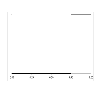
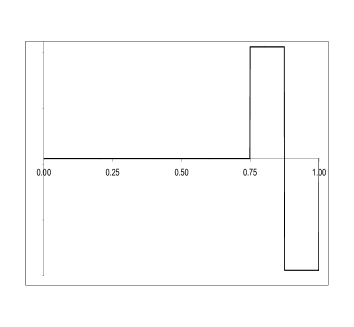
Figure 1: Scaling ($\phi_{2,3}$) and wavelet ($\psi_{2,3}$) functions.

4 Haar wavelets approximation

Let us mention an issue regarding the CDF $\overline{F}$ defined above. Since the loss can take only a finite number of discrete values ($2^{N}$ at most) the PDF of the loss function is a sum of Dirac delta functions and then, the CDF is a discontinuous function. Moreover, the stepped form of the CDF makes the Haar wavelets a natural and very well-suited way of approximation.

4.1 Laplace Transform Inversion

Due to the fact that $\overline{F}\in L^{2}([0,1])$ and according to the theory of MRA, we can approximate $\overline{F}$ in $[0,1]$ by a sum of scaling functions,

$$\overline{F}(x)\approx\sum_{k=0}^{2^{m}-1}c_{m,k}\phi_{m,k}(x),$$ (2)

and

$$\overline{F}(x)=\lim_{m\rightarrow+\infty}\sum_{k=0}^{2^{m}-1}c_{m,k}\phi_{m,k}(x).$$

Recall that in the one-factor model framework, if the systematic factor $Y$ is fixed, default occurs independently because the only remaining uncertainty is the idiosyncratic risk. The MGF conditional on $Y$ is thus given by the product of each obligor’s MGF as

$$\begin{split}M_{L}(s;Y)\equiv\mathbb{E}(e^{-sL}\mid Y)&=\prod_{n=1}^{N}\mathbb{E}\left(e^{-sE_{n}D_{n}}\mid Y\right)\\ &=\prod_{n=1}^{N}\left[1-p_{n}(y)+p_{n}(y)e^{-sE_{n}}\right].\end{split}$$

Notice that we are assuming non stochastic LGD. Taking the expectation value of this conditional MGF yields the unconditional MGF,

$$\begin{split}M_{L}(s)\equiv\mathbb{E}(e^{-sL})&=\mathbb{E}(\mathbb{E}(e^{-sL}\mid Y))\\ &=\mathbb{E}(M_{L}(s;Y))=\mathbb{E}\left[\prod_{n=1}^{N}\left[1-p_{n}(y)+p_{n}(y)e^{-sE_{n}}\right]\right]\\ &=\int_{\mathbb{R}}\prod_{n=1}^{N}\left[1-p_{n}(y)+p_{n}(y)e^{-sE_{n}}\right]\frac{1}{\sqrt{2\pi}}e^{-\frac{y^{2}}{2}}dy.\end{split}$$

But if $f$ is the probability density function of the loss function then the unconditional MGF is also the Laplace transform of $f$:

$$M_{L}(s)\equiv\mathbb{E}(e^{-sL})=\int_{0}^{+\infty}e^{-sx}f(x)dx=\widetilde{f}(s).$$ (3)

As we have noticed before,

$$f(x)=\sum_{i=0}^{2^{N}}\mu_{i}\delta(x-x_{i}),\hskip 28.45274ptx_{1},x_{2},...,x_{2^{N}}\in[0,1].$$ (4)

where $\delta(x-x_{i})$ is the Dirac delta at $x_{i}$ that can be thought as a density distribution of a unit of mass concentrated in the point $x_{i}$ (i.e. $\int_{0}^{+\infty}g(x)\delta(x-x_{i})dx=g(x_{i})$, for every test function $g(x)$). Probabilistically, a distribution, such as (4), corresponds to a situation where only the scenarios $x_{1},x_{2},...,x_{2^{N}}$ are feasible with respective probabilities $\mu_{1},\mu_{2},...,\mu_{2^{N}}$. Of course these probabilities must be positive and sum up 1, this is,

$$\sum_{i=0}^{2^{N}}\mu_{i}=1.$$

As it is also well known, in the context of generalized functions, the derivative of the Heaviside step function is a Dirac delta. In this context (and of course in the context of regular functions) we can integrate by parts the expression (3) and using the approximation (2) to conclude that,

$$\begin{split}M_{L}(s)&=\int_{0}^{+\infty}e^{-sx}F^{\prime}(x)dx=e^{-s}+s\int_{0}^{1}e^{-sx}\overline{F}(x)dx\\ &\approx e^{-s}+s\int_{0}^{1}\left[e^{-sx}\sum_{k=0}^{2^{m}-1}c_{m,k}\phi_{m,k}(x)\right]dx\\ &=e^{-s}+2^{\frac{m}{2}}s\sum_{k=0}^{2^{m}-1}c_{m,k}\widetilde{\phi}_{m,k}(s),\end{split}$$ (5)

where

$$\widetilde{\phi}_{m,k}(s)=\frac{1}{s}e^{-s\frac{k}{2^{m}}}(1-e^{-s\frac{1}{2^{m}}}).$$

is the Laplace transform of the basis function $\phi_{m,k}(x)$.

Observing that $\widetilde{\phi}_{m,k}(s)=\widetilde{\phi}_{m,0}(s)e^{-s\frac{k}{2^{m}}}$ and making the change of variable $z=e^{-s\frac{1}{2^{m}}}$, the expression (5) is the same as

$$Q(z)\equiv\sum_{k=0}^{2^{m}-1}c_{m,k}z^{k}\approx\frac{M_{L}(-2^{m}ln(z))-z^{2^{m}}}{2^{\frac{m}{2}}(1-z)}.$$ (6)

Where we note that for $r<1$, $Q(z)$ is analytic inside the disc of the complex plane $\{z:\left|z\right|<r\}$, since the singularity in $z=0$ is avoidable. Then, given the generating function $Q(z)$, we can obtain expressions for the coefficients $c_{m,k}$ by means of the Cauchy’s integral formula. This is,

$$c_{m,k}=\frac{1}{2\pi i}\int_{\gamma}\frac{Q(z)}{z^{k+1}}dz,\hskip 28.45274ptk=0,1,...,2^{m}-1.$$

where $\gamma$ is a circle about the origin of radius $r$, $0<r<1$.

Making the change of variable $z=re^{iu}$, $0<r<1$,

$$\begin{split}c_{m,k}=\frac{1}{2\pi r^{k}}\int_{0}^{2\pi}\frac{Q(re^{iu})}{e^{iku}}du&=\frac{1}{2\pi r^{k}}\int_{0}^{2\pi}\left[Re(Q(re^{iu}))cos(ku)+Im(Q(re^{iu}))sin(ku)\right]du\\ &=\frac{2}{\pi r^{k}}\int_{0}^{\pi}Re(Q(re^{iu}))cos(ku)du.\end{split}$$ (7)

Finally, we can calculate the integral in (7) approximately by means of the trapezoidal rule to obtain the coefficients.

4.2 VaR computation

It can be easily proved that

$$0\leq c_{m,k}\leq 2^{-\frac{m}{2}},\hskip 28.45274ptk=0,1,...,2^{m}-1,$$

and

$$0\leq c_{m,0}\leq c_{m,1}\leq...\leq c_{m,2^{m}-1}.$$

VaR can now be calculated quickly with at most $m$ coefficients for each fixed level of resolution $m$ of the approximation, due to the compact support of the basis functions. Observe that

$$\overline{F}(l_{\alpha})=2^{\frac{m}{2}}\cdot c_{m,k}\hskip 28.45274pt\frac{k}{2^{m}}\leq l_{\alpha}\leq\frac{k+1}{2^{m}}$$

Thus, we can simply start searching $l_{\alpha}$ computing $\overline{F}(\frac{2^{m-1}}{2^{m}})$ with any bisection like method. If $\overline{F}(\frac{2^{m-1}}{2^{m}})>\alpha$ then we compute $\overline{F}(\frac{2^{m-1}-2^{m-2}}{2^{m}})$, otherwise we compute $\overline{F}(\frac{2^{m-1}+2^{m-2}}{2^{m}})$, and so on. Finally, observe that VaR lies between $\frac{k}{2^{m}}$ and $\frac{k+1}{2^{m}}$ for a certain $k\in\{0,1,...,2^{m-1}\}$.

5 Numerical Examples

In this section we present a comparative study to calculate VaR between the Wavelet Approximation (WA) method and Monte Carlo (MC). As it is well known, MC has a strong dependence between the size of the portfolio and the computational time. As the size increases, MC becomes a big time consuming method.

The real situation in some financial companies show us that there are strong concentrations in their credit portfolios. Basel II formulas to calculate VaR are supported under unrealistic hypothesis, such as infinite number of obligors with small exposures.

For these reasons, we test our methodology with concentrated portfolios. We consider four portfolios ranging from 100 to 10000 obligors with the main numerical results displayed in Table 1. The Wavelet Approximation with $m=10$ provides accurate results in a few seconds of computational time, since the maximum relative error $(\max\left|\hbox{WA}\hbox{WA}\right|/MC)$ in portfolios P1, P2 and P3 is only 0.5%, 1% and 0.7% respectively. The relative error in portfolio P4 may look somewhat greater than expected (2.5%). But in this case, performing $5\times 10^{5}$ MC simulations we find that the VaR obtained is 0.160, being the maximum relative error of 1.2% and showing again the fast convergence of the WA methodology.

Figure 2: Tail probability approximation of portfolio P1 with $m=7$.

Finally, in order to display the accuracy of Wavelet Approximation, we have considered the tail probabilities of the loss function associated with portfolio P1 using different resolutions ($m=7,8,9$ and 10). The results, compared again with Monte Carlo simulations, can be seen in figures 2,3,4 and 5 respectively. It is remarkable how the Haar wavelets are naturally capable of detecting jumps in the cumulative distribution, making the approximation very precise with not many terms.

Portfolio	N	$P_{n}$	WA $(m=9)$	WA $(m=10)$	MC
P1	100	0.21%	$[0.193,0.195)$	$[0.194,0.195)$	0.194
P2	1000	1.00%	$[0.191,0.193)$	$[0.192,0.193)$	0.194
P3	1000	0.30%	$[0.139,0.141)$	$[0.140,0.141)$	0.141
P4	10000	1.00%	$[0.160,0.162)$	$[0.161,0.162)$	0.158

Table 1: Results of 99.9% VaR computation with Wavelet Approximation and Monte Carlo simulations with $2\times 10^{5}$ random scenarios and $\rho=0.15$. In order to consider concentrated portfolios, in all cases we have taken $E_{n}=\frac{C}{n}$ where $C$ is a constant such that $\sum_{n=1}^{N}E_{n}=1$.

Figure 3: Tail probability approximation of portfolio P1 with $m=8$.

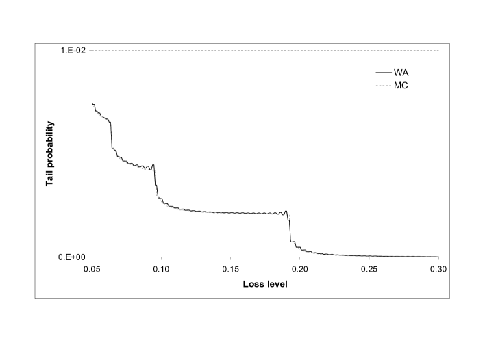
Figure 4: Tail probability approximation of portfolio P1 with $m=9$.

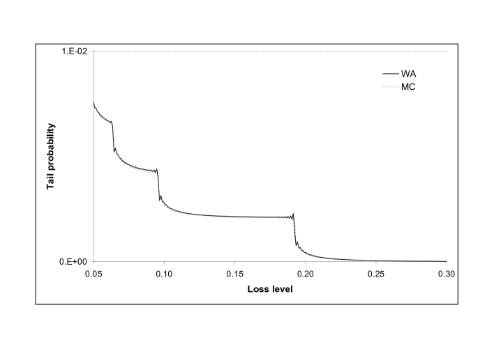
Figure 5: Tail probability approximation of portfolio P1 with $m=10$.

6 Conclusions

We have presented a numerical approximation to the loss function based on Haar wavelets system. First of all, we approximate the discontinuous distribution of the loss function by a finite sum of Haar scaling functions, and then we calculate the coefficients of the approximation by inverting its Laplace transform. Due to the compact support property of Haar system, only a few coefficients are needed for VaR computation.

We have shown the performance of the numerical approximation in four sample portfolios. These results among other simulations, show that the method is applicable to different sized portfolios and very accurate with short time computations. Moreover, the Wavelet Approximation is robust since the method is very stable under changes in the parameters of the model. The stepped form of the approximated distribution makes the Haar wavelets natural and very suitable for the approximation.

We also remark that the algorithm is valid for continuous cumulative distribution functions, and that it can be used in other financial models without making conceptual changes in the development. For instance, we can easily introduce stochastic loss given default (just changing a bit the unconditional moment generating function) and consider the multi-factor Merton model as the model framework as well.

References

- [Aba96] J. Abate, G.L. Choudhury and W. Whitt (2000). On the Laguerre method for numerically inverting Laplace transforms. Journal on Computing.
- [Aba00] J. Abate, G.L. Choudhury and W. Whitt (2000). An introduction to numerical transform inversion and its application to probability models. Computational Probability, ed. W.K. Grassman, Kluwer, Norwell, MA.
- [Ahn03] J. Ahn, S. Kang and Y. Kwon (2003). A flexible inverse Laplace transform algorithm and its application. Computing 71. 115-131.
- [Art97] P. Artzner, F. Delbaen, J.M. Eber, D. Heath (1997). Thinking coherently. RISK (November), 68-71.
- [Art99] P. Artzner, F. Delbaen, J.M. Eber, D. Heath (1999). Coherent measures of risk. Mathematical Finance 9 (3): 203-228.
- [Dau92] I. Daubechies (1992). Ten lectures on wavelets. CBMS-NSF Regional Conference Series in Applied Mathematics. SIAM.
- [Gie06] G. Giese (2006). A saddle for complex credit portfolio models. RISK (July), 84-89.
- [Gla05] P. Glasserman and J. Li (2005). Importance sampling for credit portfolios. Management Science, 51(11). 1643-1656.
- [Gla07] P. Glasserman and J. Ruiz-Mata (2007). Computing the credit loss distribution in the Gaussian copula model: a comparison of methods. Journal of Credit Risk 3. 33-66.
- [Hoo82] F. de Hoog, J. Knight and A. Stokes (1982). An improved method for numerical inversion of Laplace transforms. SIAM Journal on Scientific and Statistical Computing 3. 357-366.
- [Kal94] M. Kalkbrener (2004). Sensible and efficient capital allocation for credit portfolios. RISK (January), S19-S24.
- [Mar01a] R. Martin, K. Thompson and C. Browne (2001). Taking to the saddle. RISK (June), 91-94.
- [Mar01b] R. Martin, K. Thompson and C. Browne (2001). How dependent are defaults. RISK (July), 87-90.
- [Mar01c] R. Martin, K. Thompson and C. Browne (2001). VaR: who contributes and how much?. RISK (August), 99-102.
- [Mar04] R. Martin (2004). Credit portfolio modeling handbook. Credit Suisse First Boston Limited.
- [Mar06] R. Martin and R. Ordovás (2006). An indirect view from the saddle. RISK (October), 94-99.
- [Tak08] Y. Takano and J. Hashiba (2008). A novel methodology for credit portfolio analysis: numerical approximation approach. www.defaultrisk.com.