Analytical Models of the Intergalactic Medium and Reionization

Abstract

Reionization is a process whereby hydrogen (and helium) in the Universe is ionized by the radiation from first luminous sources. Theoretically, the importance of the reionization lies in its close coupling with the formation of first cosmic structures and hence there is considerable effort in modelling the process. We give a pedagogic overview of different analytical approaches used for modelling reionization. We also discuss different observations related to reionization and show how to use them for constraining the reionization history.

I Introduction

Current models of cosmology dkn++09 indicate that about three-fourth of the energy density in our present Universe is constituted by “dark energy” which is responsible for the current acceleration of the cosmic expansion. The next dominant component is the “dark matter” which constitutes about 23 per cent of the density. This form of matter is collisionless and interact only gravitationally. The baryons constitute only 2 per cent of the total mass. The two most abundant elements among the baryons are hydrogen and helium.

Study of reionization mostly concerns with the ionization and thermal history of the baryons (hydrogen and helium) in our Universe lb01 ; bl01 ; cf06a ; fck06 . Within the framework of hot Big Bang model, hydrogen formed for the first time when the age of the Universe was about $3\times 10^{5}$ years, its size being one-thousandth of the present (corresponding to a scale factor $a\approx 0.001$ and a redshift $z=1/a-1\approx 1000$). Around this time, the temperature of the radiation became low enough $\approx 3\times 10^{3}$ K that the photons were not able to ionize the proton-electron pair through collisions and hence formation of hydrogen (and some amount of helium) could take place peebles93 . The epoch at which the protons and the electrons combined for the first time to form hydrogen atoms is known as the recombination epoch and is well-probed by the Cosmic Microwave Background Radiation (CMBR).

Right after the recombination epoch, the Universe entered a phase called the “dark ages” where no significant radiation sources existed. The hydrogen remained largely neutral at this phase. The small inhomogeneities in the dark matter density field which were present during the recombination epoch started growing via gravitational instability giving rise to highly nonlinear structures like the collapsed haloes cr86 . It should, however, be kept in mind that most of the baryons at high redshifts do not reside within these haloes, they rather reside as diffuse gas within the intergalactic space which is known as the intergalactic medium (IGM) peacock99 ; padmanabhan02b .

The collapsed haloes form potential wells whose depth depend on their mass and the baryons (i.e, hydrogen) then “fall” in these wells. If the mass of the halo is high enough (i.e., the potential well is deep enough), the gas will be able to dissipate its energy, cool via atomic or molecular transitions and fragment within the halo. This produces conditions appropriate for condensation of gas and forming stars and galaxies. Once these luminous objects form, the era of dark ages can be thought of being over.

The first population of luminous stars and galaxies can generate ultraviolet (UV) radiation through nuclear reactions. In addition to the galaxies, perhaps an early population of accreting black holes (quasars) also generated some amount UV radiation. The UV radiation contains photons with energies $>13.6$ eV which are then able to ionize hydrogen atoms in the surrounding medium, a process known as “reionization”. Reionization is thus the second major change in the ionization state of hydrogen (and helium) in the Universe (the first being the recombination).

As per our current understanding gnedin00 ; wl03 ; cf06b , reionization started around the time when first structures formed, which is currently believed to be around $z\approx 20-30$. In the simplest picture, each source first produced an ionized region around it; these regions then overlapped and percolated into the IGM. This era is usually called the “pre-overlap” phase. The process of overlapping seemed to be completed around $z\approx 6-8$ at which point the neutral hydrogen fraction fell to values lower than $10^{-4}$. Following that a never-ending “post-reionization” (or “post-overlap”) phase started which implies that the Universe is largely ionized at present epoch. Reionization by UV radiation is also accompanied by heating: electron which are released by photoionization will deposit an extra energy equivalent to $h_{p}\nu-13.6~{}{\rm eV}$ to the IGM, where $\nu$ is the frequency of the ionizing photon and $h_{p}$ is the Planck constant. This reheating of the IGM can expel the gas and/or suppress cooling in the low mass haloes – thus, there is a considerable reduction in the cosmic star formation right after reionization. In addition, the nuclear reactions within the stellar sources potentially alter the chemical composition of the medium if the star dies via energetic explosion (supernova). This can change the nature of star formation at later stages.

The process of reionization is of immense importance in the study of structure formation since, on one hand, it is a direct consequence of the formation of first structures and luminous sources while, on the other, it affects subsequent structure formation. Observationally, the reionization era represents a phase of the Universe which is yet to be probed; the earlier phases ($z\approx 1000$) are probed by the CMBR while the post-reionization phase ($z<6$) is probed by various observations based on galaxies, clusters, quasars and other sources. In addition to the importance outlined above, the study of dark ages and cosmic reionization has acquired increasing significance over the last few years because of the availability of good quality data in different areas.

In this article, we will mainly concentrate on the current status of various analytical and semi-analytical approaches which go into modelling reionization. The main aim would be to systematically discuss the set of equations which are crucial in understanding the process highlighting the major physical processes and assumptions. We shall also highlight the relevant observational probes at appropriate places. In Section II, we shall give a pedagogic introduction to the basic theoretical formalism for studying reionization and IGM in different phases of evolution. Section III would be devoted to discussing detailed modelling of reionization using the formalism developed. We shall illustrate on how to constrain the models by comparing with a wide variety of available data sets. In Section IV, we shall briefly discuss the current numerical simulations and observations related to reionization. We shall also highlight what to expect in this field in near future.

II Theoretical Formalism

In this section, we discuss the basic theoretical formalism required for modelling reionization of the IGM. The main aim here would be to highlight the physical processes which are crucial in understanding reionization and comparing with observations. In what follows, we shall assume that the IGM consists only of hydrogen and neglect the presence of helium. It is straightforward to include helium into the formalism.

Essentially, in presence of a ionizing radiation, the evolution of the mean neutral hydrogen density $n_{\rm HI}$ is given by

$$\dot{n}_{\rm HI}=-3H(t)n_{\rm HI}-\Gamma_{\rm HI}n_{\rm HI}+{\cal C}\alpha(T)n_{\rm HII}n_{e}$$ (1)

where overdots denote the total time derivative ${\rm d}/{\rm d}t$, $H\equiv\dot{a}/a$ is the Hubble parameter, $\Gamma_{\rm HI}$ is the photoionization rate per hydrogen atom, $\alpha(T)$ is the recombination rate coefficient and $n_{e}$ represents the mean electron density. The first term in the right hand side of equation (1) corresponds to the dilution in the density because of cosmic expansion, the second term corresponds to photoionization by the ionizing flux and the third term corresponds to recombination of protons and free electrons into neutral hydrogen. The quantity ${\cal C}$ is called the clumping factor and is defined as

$${\cal C}\equiv\frac{\langle n_{\rm HII}n_{e}\rangle}{\langle n_{\rm HII}\rangle\langle n_{e}\rangle}=\frac{\langle n_{H}^{2}\rangle}{\langle n_{H}\rangle^{2}}$$ (2)

where the last equality holds for the case when the IGM contains only hydrogen (i.e., no helium) and is highly ionized, i.e, $n_{e}=n_{\rm HII}\approx n_{H}$. The clumping factor takes into account the fact that the recombination rate in an inhomogeneous (clumpy) IGM is higher than a medium of uniform density.

The ionization equation is usually supplemented by the evolution of the IGM temperature $T$, which is given by

$$\dot{E}_{\rm kin}=-2H(t)E_{\rm kin}+\Lambda$$ (3)

where $E_{\rm kin}=3k_{B}Tn_{H}$ is the kinetic energy of the gas and $\Lambda$ is the net heating rate including all possible heating and cooling processes. The first term on the right hand side takes into account the adiabatic cooling of the gas because of cosmic expansion.

II.1 Cosmological radiation transfer

The equation of radiation transfer, which describes propagation of radiation flux through a medium, is written as an evolution equation for the specific intensity of radiation $I_{\nu}\equiv I(t,{\bf x},\nu,{\bf\hat{n}})$ which has dimensions of the energy per unit time per unit area per unit solid angle per frequency range. It is a function of time and space coordinates $(t,{\bf x})$, the frequency of radiation $\nu$ and the direction of propagation ${\bf\hat{n}}$. The radiation transfer equation in a cosmological scenario has the form anm99

$$\frac{\partial I_{\nu}}{\partial t}+\frac{c}{a(t)}{\bf\hat{n}\cdot\nabla_{x}}I_{\nu}-H(t)\nu\frac{\partial I_{\nu}}{\partial\nu}+3H(t)I_{\nu}$$

$$=-c\kappa_{\nu}I_{\nu}+\frac{c}{4\pi}\epsilon_{\nu},$$ (4)

where $\kappa_{\nu}$ is the absorption coefficient and $\epsilon_{\nu}$ is the emissivity. The above equation is essentially the Boltzmann equation for photons with $I_{\nu}$ being directly proportional to the phase space distribution function padmanabhan02b . The terms on the left hand side of equation (4) add up to the total time derivative of $I_{\nu}$; in particular, the third term corresponds to dilution of the intensity and the fourth term accounts for shift of frequency $\nu\propto a^{-1}$ because of cosmic expansion. The effect of scattering (which is much rarer than absorption in the IGM) can, in principle, be included in the $\kappa_{\nu}$ term if required. If the medium contains absorbers with number density $n_{\rm abs}$ each having a cross-section $\sigma_{\nu}$, the absorption coefficient is given by $\kappa_{\nu}=n_{\rm abs}\sigma_{\nu}$. The mean free path of photons in the medium is given by $\lambda_{\nu}(t)\equiv\kappa^{-1}_{\nu}(t)$.

We define the mean specific intensity by averaging $I_{\nu}$ over a large volume and over all directions

$$J_{\nu}(t)\equiv\int_{V}\frac{{\rm d}^{3}x}{V}\int\frac{{\rm d}\Omega}{4\pi}I_{\nu}(t,{\bf x},{\bf\hat{n}})$$ (5)

Then the spatially and angular-averaged radiation transfer equation becomes peebles93

$$\dot{J}_{\nu}\equiv\frac{\partial J_{\nu}}{\partial t}-H(t)\nu\frac{\partial J_{\nu}}{\partial\nu}=-3H(t)J_{\nu}-c\kappa_{\nu}J_{\nu}+\frac{c}{4\pi}\epsilon_{\nu}$$ (6)

where the coefficients $\kappa_{\nu}$ and $\epsilon_{\nu}$ are now assumed to be averaged over the large volume. The quantity $J_{\nu}$ is essentially the energy per unit time per unit area per frequency interval per solid angle.

The integral solution of the above equation along a line of sight can be written as hm96

$$J_{\nu}(t)=\frac{c}{4\pi}\int_{0}^{t}{\rm d}t^{\prime}\epsilon_{\nu^{\prime}}(t^{\prime})\left[\frac{a^{3}(t^{\prime})}{a^{3}(t)}\right]{\rm e}^{-\tau(t,t^{\prime};\nu)}.$$ (7)

where $\nu^{\prime}=\nu a(t)/a(t^{\prime})$, $\nu^{\prime\prime}=\nu a(t)/a(t^{\prime\prime})$ and

$$\tau(t,t^{\prime};\nu)\equiv c\int_{t^{\prime}}^{t}{\rm d}t^{\prime\prime}\kappa_{\nu^{\prime\prime}}(t^{\prime\prime})=c\int_{t^{\prime}}^{t}\frac{{\rm d}t^{\prime\prime}}{\lambda_{\nu^{\prime\prime}}(t^{\prime\prime})}$$ (8)

is the optical depth along the line of sight from $t^{\prime}$ to $t>t^{\prime}$ Clearly, the intensity at a given epoch is proportional to the integrated emissivity with an exponential attenuation due to absorption in the medium. The intensity attenuates by $1/{\rm e}$ when the radiation travels a distance equal to the mean free path.

The absorption is “local” when the mean free path of photons is much smaller than the horizon size of the Universe, i.e., $\lambda_{\nu}(t)\ll c/H(t)$. In addition, if we also assume that the emissivity $\epsilon_{\nu}$ does not evolve significantly over the small time interval $\lambda/c$, then the specific intensity is related to the emissivity through a simple form mhr99 ; mhr00

$$J_{\nu}(t)\approx\frac{\epsilon_{\nu}(t)\lambda_{\nu}(t)}{4\pi}=\frac{\epsilon_{\nu}(t)}{4\pi\kappa_{\nu}(t)}$$ (9)

Note that in the case of local absorption, $\dot{J},HJ\ll c\epsilon$. In this approximation, the background intensity depends only on the instantaneous value of the emissivity (and not its history) because all the photons are absorbed shortly after being emitted (unless the sources evolve synchronously over a timescale much shorter than the Hubble time). We shall discuss later in Section II.2 that this is a useful approximation for the IGM for redshifts $z\gtrsim 3$.

II.2 Post-reionization epoch

Let is first study the radiation transfer in the post-reionization epoch. Compared to the pre-overlap era, this epoch is much easier to study because the IGM can be treated as a highly ionized single-phase medium (whereas during the pre-overlap era, one is looking into two distinct phases – ionized and neutral). The optical depth can be written as

$$\tau(z,z^{\prime};\nu)=c\int_{z}^{z^{\prime}}\frac{{\rm d}z^{\prime\prime}}{(1+z^{\prime\prime})H(z^{\prime\prime})}n_{\rm HI}(z^{\prime\prime})~{}\sigma_{\rm abs}(\nu^{\prime\prime})$$ (10)

where $\sigma_{\rm abs}(\nu)$ is the total absorption cross section of neutral hydrogen and we have changed the time coordinate to the redshift $z$. Various processes can, in principle, contribute to $\sigma_{\rm abs}(\nu)$, most dominant being the resonant Lyman series absorption corresponding to excitation of hydrogen atoms from the ground state to higher ones (1s $\to n$p) and the continuum absorption of photons above the ionization threshold via photoionization process. Let us treat each of them separately in the following:

II.2.1 Resonant Lyman series absorption

The Lyman series absorption arises from the electronic excitation of neutral hydrogen atoms from the 1s ground state to higher ones. The most dominant of these are the Ly$\alpha$ (1s $\to$ 2p, rest wavelength $\lambda_{\alpha}\approx 1216\AA\$) and Ly$\beta$ (1s $\to$ 3p, $\lambda_{\beta}\approx 1206\AA\$) transitions, and hence they are the most relevant ones as far as observations are concerned. For simplicity, we shall present results for the Ly$\alpha$ absorption only, the others can be calculated in identical manner. The Ly$\alpha$ absorption cross section is given by

$$\sigma_{\rm abs}(\nu)=\sigma_{\alpha}~{}V\left(\frac{\nu}{\nu_{\alpha}}-1\right)$$ (11)

where $\nu_{\alpha}=c/\lambda_{\alpha}$ is the resonant frequency of transition, $\sigma_{\alpha}=4.45\times 10^{-18}{\rm cm}^{2}$ is the cross section at $\nu_{\rm alpha}$ and $V$ is a function which determines the profile of the absorption line. It is called the Voigt profile function and is a convolution of the Lorentzian shape for the natural broadening and the Gaussian shape for the thermal broadening. For the purpose of this article, it is sufficient to note that $V$ is a sharply peaked function about $\nu/\nu_{\alpha}=1$; for most our discussion, we shall take it to be a Dirac-delta function $V(\nu/\nu_{\alpha}-1)=\delta_{D}(\nu/\nu_{\alpha}-1)$.

The optical depth between the redshifts $z$ and $z^{\prime}$ is then given by

$$\tau(z,z^{\prime};\nu)=\tau(z_{\alpha})=\sigma_{\alpha}\frac{c}{H(z_{\alpha})}n_{\rm HI}(z_{\alpha});$$

$$1+z_{\alpha}=\frac{\nu_{\alpha}}{\nu}(1+z)$$ (12)

If we put this into equation (7), we see that the Ly$\alpha$ absorption at a redshift $z_{\alpha}$ reduces the specific intensity observed at $z$ at a frequency $\nu_{\alpha}(1+z)/(1+z_{\alpha})$ by a factor $e^{-\tau(z_{\alpha})}$. The value of $\tau(z_{\alpha})$ along a given line of sight would depend upon the distribution of $n_{\rm HI}(z_{\alpha})$. However, we would mostly be interested in the mean value of specific intensity averaged over a number of lines of sight. The corresponding reduction can be described by a line-of-sight-averaged optical depth

$${\rm e}^{-\tau_{\rm eff}(z_{\alpha})}\equiv\langle{\rm e}^{-\tau(z_{\alpha})}\rangle_{\rm LOS}$$ (13)

where $\langle~{}\rangle_{\rm LOS}$ denotes averaging over lines of sight. The quantity $\tau_{\rm eff}$ is usually known as the “effective optical depth”.

Theoretically, the value of $\tau_{\rm eff}$ can be calculated if we know the distribution of optical depth $P(\tau)$ [which can be calculated from the neutral hydrogen distribution $P(n_{\rm HI})$]:

$${\rm e}^{-\tau_{\rm eff}(z)}=\int_{0}^{\infty}{\rm d}\tau~{}P(\tau;z)~{}{\rm e}^{-\tau}$$ (14)

Of course, one requires detailed understanding of the evolution of the baryonic density field to model the distribution $P(n_{\rm HI})$. This has been addressed by a series of analytical studies bbc92 ; bi93 ; gh96 ; bd97 ; hgz97 ; gh98 ; mhr00 ; cps01 ; csp01 and numerical simulations cmor94 ; zan95 ; hkwm96 ; mcor96 ; vmmth02 ; msc++05 ; bhvs05 ; msb++06 ; bvkhc08 , which we shall avoid discussing here. However, we can still make some inference assuming the distribution is uniform, i.e., $\tau_{\rm eff}(z)=c\sigma_{\alpha}n_{\rm HI}(z)/H(z)$. If we define the neutral hydrogen fraction to be $x_{\rm HI}\equiv n_{\rm HI}/n_{H}$, then we can calculate $\tau_{\rm eff}\propto x_{\rm HI}$ given a set of cosmological parameters (which would uniquely determine $H(z)$ and $n_{H}$).

Figure 1: The effective optical depth of Ly$\alpha$ absorption as function of redshift $z$. The points with errorbars represent the observational data. The dashed curves, from top to bottom, represent the predictions for a uniform IGM with neutral hydrogen fraction $x_{\rm HI}=(3,1,0.3)\times 10^{-5}$, respectively.

Observationally, $\tau_{\rm eff}$ can be determined by looking at the spectra of bright sources like quasars at high redshifts. These spectra show a series of absorption features at frequencies larger than the Ly$\alpha$ frequency in the quasar rest frame. Since one has a good knowledge of the unabsorbed quasar spectra (from looking at nearby quasars and also having some understanding about the physical processes), one can calculate the amount of absorption happening because of the intervening IGM between the quasar and the observer; this absorption, averaged over numerous lines of sight, is essentially the quantity ${\rm e}^{-\tau_{\rm eff}}$. This has been done to quite high redshifts $z\sim 6.5$ and the values of $\tau_{\rm eff}$ observed are shown as points with errorbars songaila04 ; fsb++06 in Figure 1.

To understand what these values imply, we have plotted with dashed lines the calculated value of $\tau_{\rm eff}$ for a uniform IGM assuming three values of $x_{\rm HI}=(3,1,0.3)\times 10^{-5}$ from top to bottom. This immediately tells us that the fraction of neutral hydrogen has to be $\sim 10^{-5}$ in order to reproduce the observed values of $\tau_{\rm eff}$. In fact, had $x_{\rm HI}$ been slightly (say $\sim 10^{-4}$) higher, one would have obtained $\tau_{\rm eff}$ much higher than unity ($\sim 10-100$) and hence the flux from the quasar would be completely absorbed. If that were the case, it would show up as a absorption “trough” at frequencies larger than the rest frame Ly$\alpha$ frequency. In reality, a considerable amount of transmitted flux is found at these frequencies alongwith a series of absorption features arising from the Ly$\alpha$ transition of residual neutral hydrogen. These absorption signatures are known as the “Ly$\alpha$” forest and are powerful probes of the neutral hydrogen distribution in the IGM at $z<6$ rauch98 .

The absence of a absorption trough is a direct proof of the fact that hydrogen is completely reionized in the diffuse IGM at redshifts $z\lesssim 6$. This is known as the Gunn-Peterson effect gp65 . Note that the actual inferred value of $x_{\rm HI}$ might be slightly different if one models with an appropriate density distribution, however, the basic conclusion remains unchanged.

We can also see from Figure 1 that for quasars at redshifts $z\gtrsim 6$, the observed value of $\tau_{\rm eff}\gtrsim 5$; this would imply an attenuation $\gtrsim 0.01$ and hence one actually observes absorption troughs as predicted by Gunn-Peterson effect fsb++06 ; wdr++09 . Unfortunately, finding such troughs does not necessarily imply that the IGM is highly neutral as even a $x_{\rm HI}\sim 10^{-4}$ could be sufficient to absorb all the flux. However, one can use much detailed modelling to improve the constraint, which we shall discuss later in Section III.2.

The values of $\tau_{\rm eff}\lesssim 1$ at $z<4$ means that the diffuse IGM is highly transparent (also called optically thin) to Ly$\alpha$ photons. Only about $\sim 10\%$ of the Ly$\alpha$ photons are absorbed, mostly within the high density regions. These high density systems are often modelled as a set of discrete absorbers of some size. If we consider an absorber having neutral hydrogen density $n_{\rm HI}$ and a size $L\ll c/H(z)$ along the line of sight at a redshift $z_{\rm abs}$, the optical depth is given by

$$\tau(z,z^{\prime};\nu)=N_{\rm HI}~{}\sigma_{\rm abs}(\nu_{\rm abs})$$ (15)

where $\nu_{\rm abs}=\nu(1+z_{\rm abs})/(1+z)$ and $N_{\rm HI}\equiv n_{\rm HI}~{}L$ is the column density of neutral hydrogen within the absorber. Hence, each absorber reduces the specific intesnity by a factor ${\rm e}^{-N_{\rm HI}\sigma_{\rm abs}(\nu_{\rm abs})}$. If we assume that the absorbers are Poisson-distributed, then it is straightforward to show that the effective optical depth is given by pmb80

$$\tau_{\rm eff}(z,z^{\prime};\nu)=$$

$$\int_{z}^{z^{\prime}}{\rm d}z^{\prime\prime}\int_{0}^{\infty}{\rm d}N_{\rm HI}\frac{\partial^{2}N}{\partial z^{\prime\prime}\partial N_{\rm HI}}[1-{\rm e}^{-N_{\rm HI}\sigma_{\rm abs}(\nu^{\prime\prime})}]$$ (16)

where $[\partial^{2}N/\partial z\partial N_{\rm HI}]~{}{\rm d}z~{}{\rm d}N_{\rm HI}$ is the number of absorbers within $(z,z+{\rm d}z)$ having column densities in the range $(N_{\rm HI},N_{\rm HI}+{\rm d}N_{\rm HI})$.

In case of Ly$\alpha$ resonant absorption, we can use the cross section in (11) to calculate $\tau_{\rm eff}$. Since $V$ is a function which is sharply peaked around $\nu/\nu_{\alpha}=1$, we can approxiamte the above integral as

$$\tau_{\rm eff}(z,z^{\prime};\nu)=\frac{1+z_{\alpha}}{\lambda_{\alpha}}\int_{0}^{\infty}{\rm d}N_{\rm HI}\frac{\partial^{2}N}{\partial z_{\alpha}\partial N_{\rm HI}}W_{\alpha}(N_{\rm HI})$$ (17)

where

$$W_{\alpha}(N_{\rm HI})\equiv\int{\rm d}\lambda^{\prime\prime}\left[1-{\rm e}^{-N_{\rm HI}\sigma_{\alpha}V(\lambda_{\alpha}/\lambda^{\prime\prime}-1)}\right]$$ (18)

is called the “equivalent width” of the absorber.

II.2.2 Continuum absorption

In case of continuum absorption of radiation by photoionization, the cross section is given by

$$\sigma_{\rm abs}(\nu)=\sigma_{\rm HI}(\nu)\Theta(\nu-\nu_{\rm HI})$$ (19)

where $\sigma_{\rm HI}(\nu)$ is the photoionization cross section and $\Theta$ is the Heaviside step function taking into account that only photons with frequencies $\nu>\nu_{\rm HI}=13.6~{}{\rm eV}/h_{p}$ would be absorbed by the photoionization process. The exact form of $\sigma_{\rm HI}(\nu)$ is rather complicated, however one can approximate it by a power-law of the form $\sigma_{\rm HI}(\nu)=\sigma_{0}(\nu/\nu_{\rm HI})^{-3}$ where $\sigma_{0}=6.3\times 10^{-18}{\rm cm}^{2}$.

Since $\sigma_{0}\sim\sigma_{\alpha}$, one can show that the absorption due to a diffuse IGM in this case too is negligibly small. The only significant absorption can be seen in very high density regions which have a large fraction of their hydrogen in neutral form. In that case, we can use the relations obtained for a set of Poisson-distributed absorbers in the vase of resonant transition. We essentially have an optical depth of the form (17), and the corresponding mean free path of ionizing photons due to these discrete absorbers is found to be mhr99 ; sb03 ; miralda03

$$\lambda_{\nu}(z) = \frac{c}{H(z)(1+z)}$$ (20)

$$\times \left[\int_{0}^{\infty}{\rm d}N_{\rm HI}\frac{\partial^{2}N}{\partial z\partial N_{\rm HI}}[1-{\rm e}^{-N_{\rm HI}\sigma_{\rm HI}(\nu)}]\right]^{-1}$$

At this point, let us introduce the concept of Lyman-limit systems which have column densities $N_{\rm HI}>\sigma^{-1}_{0}=1.6\times 10^{17}{\rm cm}^{-2}$; these absorbers contribute a optical depth of unity to the ionizing photons. The average distance between these systems is given by

$$\lambda_{\rm LLS}=\frac{c}{H(z)(1+z)}\left[\frac{{\rm d}N_{\rm LLS}}{{\rm d}z}\right]^{-1}$$ (21)

where ${\rm d}N_{\rm LLS}/{\rm d}z$ is the redshift distribution of the Lyman-limit systems

$$\frac{{\rm d}N_{\rm LLS}}{{\rm d}z}=\int_{1/\sigma_{\rm HI}(\nu_{\rm HI})}^{\infty}{\rm d}N_{\rm HI}\frac{\partial^{2}N}{\partial z\partial N_{\rm HI}}$$ (22)

For the observed distribution $\partial^{2}N/\partial z\partial N_{\rm HI}\propto N_{\rm HI}^{-1.5}$ pbcp93 , one can show from equations (20) and (21) that the mean free path is related to the distance and redshift distribution Lyman-limit systems as

$$\lambda_{\nu_{\rm HI}}=\frac{\lambda_{\rm LLS}}{\sqrt{\pi}}=\frac{c}{\sqrt{\pi}H(z)(1+z)~{}{\rm d}N_{\rm LLS}/{\rm d}z}.$$ (23)

The redshift distribution of Lyman-limit systems ${\rm d}N_{\rm LLS}/{\rm d}z$ is a quantity which has been measured for $2<z<4.5$ by observations of quasar absopriton spectra. Though the observational constraints are poor, one can still obtain a value ${\rm d}N_{\rm LLS}/{\rm d}z\approx 0.3(1+z)^{-1.55}$ smi96 , which in turn gives the mean free path as $\lambda_{\nu_{\rm HI}}/[c/H(z)]\approx 0.1[(1+z)/4]^{-2.55}$ Hence the mean free path of ionizing photons is much smaller than the horizon size for $z>3$, which implies that we can use the local absorption approximation at these redshifts.

We can summarise the main results of this section as: the post-reionization epoch is characterized by a highly ionized IGM as observed by the quasar absorption spectra. The IGM is largely transparent to ionizing photons at these redshifts. However, there exist regions with high column densities ($N_{\rm HI}>10^{17}{\rm cm}^{-2}$) which are optically thick to the ionizing radiation; these regions determine the photon mean free path. We shall see later how to use this information to obatin an improved model of the IGM.

II.3 Pre-overlap epoch

We now turn our attention towards the IGM in the pre-overlap era. In this era, the overlap of individual ionized regions is not complete and hence the IGM is partially ionized. So the radiation transfer equation has to be modified to account for the multi-phase nature of the IGM.

Let us define the volume filling factor of ionized regions to be $Q_{\rm HII}$; this the fraction of volume that is ionized and reionization is said to be complete when $Q_{\rm HII}=1$. Next, note that the number density of photons present in the background flux is

$$n_{J}(t)=\frac{4\pi}{c}\int_{\nu_{\rm HI}}^{\infty}{\rm d}\nu\frac{J_{\nu}}{h_{p}\nu}$$ (24)

Since there is no ionizing flux within the neutral regions (otherwise they would not remain neutral), the photoionization rate per hydrogen atom within the ionized (HII) regions is

$$\Gamma^{\rm II}_{\rm HI}=\frac{1}{Q_{\rm HII}}4\pi\int_{\nu_{\rm HI}}^{\infty}{\rm d}\nu\frac{J_{\nu}}{h_{p}\nu}\sigma_{\rm HI}(\nu)$$ (25)

where the factor $Q_{\rm HII}^{-1}$ accounts for the fact that the radiation is limited to a fraction of the total volume. The emmission rate of ionizing photons per unit volume from sources of emissivity $\epsilon_{\nu}$ is

$$\dot{n}_{\rm ph}=\int_{\nu_{\rm HI}}^{\infty}{\rm d}\nu\frac{\epsilon_{\nu}}{h_{p}\nu}$$ (26)

Then the equation of radiation transfer then becomes mhr00 ; co00

$$\dot{n}_{J} = -3H(t)n_{J}-H(t)\frac{4\pi}{c}\frac{J_{\nu_{\rm HI}}}{h_{p}}+\dot{n}_{\rm ph}$$ (27)

$$- n_{\rm HI}^{\rm II}Q_{\rm HII}\Gamma^{\rm II}_{\rm HI}-n_{\rm HII}^{\rm II}\frac{{\rm d}Q_{\rm HII}}{{\rm d}t}$$

where $n_{\rm HI}^{\rm II}$ and $n_{\rm HII}^{\rm II}$ are the number densities of neutral and ionized hydrogen within the HII regions, respectively. The first term in the right hand side of equation (27) corresponds to the dilution in density due to cosmic expansion while the second term accounts for the loss of ionizing radiation because of a photon being redshifted below the ionization edge of hydrogen $\nu_{\rm HI}$. The third term is essentially the source of ionizing photons. The fourth term accounts for the loss of photons in ionizing the residual neutral hydrogen within the ionized regions. The fifth term, which is only relevant for the pre-overlap stages, accounts for the photons which ionize hydrogen for the first time and hence increase the filling factor $Q_{\rm HII}$. For $Q_{\rm HII}=1$, equation (27) reduces to that for the post-reionization phase.

If we now assume that the photons are absorbed locally, then $\dot{J},HJ\ll c\epsilon$ and we $J_{\nu}$ is essentially given by equation (9). We can then ignore terms containing $J$ and $n_{J}$ in equation (27). This gives a equation describing the evolution of the filling factor $Q_{\rm HII}$

$$\frac{{\rm d}Q_{\rm HII}}{{\rm d}t}=\frac{\dot{n}_{\rm ph}}{n_{\rm HII}^{\rm II}}-Q_{\rm HII}\Gamma^{\rm II}_{\rm HI}$$ (28)

If we further assume photoionization equilibrium within the ionized region ${\rm d}(n_{\rm HI}^{II}a^{3})/{\rm d}t\to 0$, then we have from equation (1) $n_{\rm HI}^{\rm II}\Gamma^{\rm II}_{\rm HI}={\cal C}\alpha(T)n_{\rm HII}^{\rm II}n_{e}^{\rm II}$ and the evolution of $Q_{\rm HII}$ can be written in the form mhr99

$$\frac{{\rm d}Q_{\rm HII}}{{\rm d}t}=\frac{\dot{n}_{\rm ph}}{n_{\rm HII}^{\rm II}}-Q_{\rm HII}~{}{\cal C}\alpha(T)n_{e}^{\rm II}$$ (29)

In this description, reionization is complete when $Q_{\rm HII}=1$ and equation (29) cannot be evolved further on. Clearly the assumptions of local absorption and photoionization equilibrium (both of which are reasonably accurate) has given us a equation which can be solved once we have a model for estimating $\epsilon_{\nu}$ and ${\cal C}$. Of course, there is a dependence of the recombination rate coefficient $\alpha(T)$ on temperature, however that dependence is often ignored while studying the volume filling factor. In case one is interested in temperature evolution, one has to solve equation (3) taking into account all the heating and cooling processes in the IGM, in particular, the photoheating by ionizing photons whose rate is given by

$$\Gamma_{\rm ph,HI}=4\pi\int_{\nu_{\rm HI}}^{\infty}{\rm d}\nu\frac{J_{\nu}}{h_{p}\nu}h_{p}(\nu-\nu_{\rm HI})\sigma_{\rm HI}(\nu).$$ (30)

II.4 Reionization of the inhomogenous IGM

The description of reionization in the previous section is not adequate as it does not take into account the inhomogeneities in the IGM appropriately (except for a clumping factor ${\cal C}$ in the effective recombination rate). To see this, consider the post-reionization phase where we know from observations that there exists regions of high density which are neutral; these regions are being gradually ionized and hence one would ideally like to write a equation similar to (29) for studying the post-reionization phase. Since the ionization state depends on the density, one should have to account for the density distribution of the IGM.

In order to proceed, first note that the volume filling factor may not be the appropriate quantity to study for evolution of reionization because most of the photons are consumed in regions with high densities (which might be occupying a small fraction of volume). In other words, if we neglect recomibation for the moment, we have from equation (29) that the volume filling factor $Q_{\rm HII}=\int{\rm d}t~{}\dot{n}_{\rm ph}/n_{H}=n_{\rm ph}/n_{H}$; however, in reality the photon to hydrogen ratio should be equal to the ionized mass fraction $F^{M}_{\rm HII}$, i.e., $n_{\rm ph}/n_{H}=F^{M}_{\rm HII}$. Hence, we must replace the volume filling factor by the mass filling factor in the description of the previous section, in particular equation (29) should have the form

$$\frac{{\rm d}F^{M}_{\rm HII}}{{\rm d}t}=\frac{\dot{n}_{\rm ph}}{n_{\rm HII}^{\rm II}}-F^{M}_{\rm HII}~{}{\cal C}\alpha(T)n_{e}^{\rm II}$$ (31)

One can relate $F^{M}_{\rm HII}$ to the IGM density distribution by using the fact that regions of lower densities will be ionized first, and high-density regions will remain neutral for a longer time. The main reason for this is that the recombination rate (which is $\propto n_{H}^{2}$) is higher in high-density regions where dense gas becomes neutral very quickly. If we assume that hydrogen in all regions with overdensities $\Delta<\Delta_{\rm HII}$ is ionized while the rest is neutral, then the mass ionized fraction is clearly mhr00

$$F^{M}_{\rm HII}\equiv F^{M}(\Delta_{\rm HII})=\int_{0}^{\Delta_{\rm HII}}{\rm d}\Delta~{}\Delta~{}P(\Delta)$$ (32)

where $P(\Delta)$ is the (volume-weighted) density distribution of the IGM. The term describing the effective recombination rate gets constribution only from the low desnity regions (high density neutral regions do not contribute) and is then given by

$$\alpha(T)n_{e}^{\rm II}\int_{0}^{\Delta_{\rm HII}}{\rm d}\Delta~{}\Delta^{2}~{}P(\Delta)\equiv\alpha(T)n_{e}^{\rm II}R(\Delta_{\rm HII})$$ (33)

The evolution for the mass ionized fraction is then

$$\frac{{\rm d}F^{M}(\Delta_{\rm HII})}{{\rm d}t}=\frac{\dot{n}_{\rm ph}}{n_{\rm HII}^{\rm II}}-R(\Delta_{\rm HII})\alpha(T)n_{e}^{\rm II}$$ (34)

The evolution equation essentially tracks the evolution of $\Delta_{\rm HII}$ which rises as $F^{M}(\Delta_{\rm HII})$ increases with time (i.e., more and more high density regions are getting ionized). Since the mean free path is determined by the high density regions, one should be able to relate it to the value of $\Delta_{\rm HII}$ mhr00 . It is clear that a photon will be able to travel through the low density ionized volume

$$F_{V}(\Delta_{\rm HII})=\int_{0}^{\Delta_{\rm HII}}{\rm d}\Delta~{}P(\Delta)$$ (35)

before being absorbed. When a very high fraction of volume is ionized, one can assume that the fraction of volume filled up by the high density regions is $1-F_{V}$, hence their size is proportional to $(1-F_{V})^{1/3}$, and the separation between them along a random line of sight will be proportional to $(1-F_{V})^{-2/3}$, which, in turn, will determine the mean free path. Then one has

$$\lambda_{\nu}(a)=\frac{\lambda_{0}}{[1-F_{V}(\Delta_{\rm HII})]^{2/3}}$$ (36)

where we can fix $\lambda_{0}$ by comparing with low redshift observations like the distribution of Lyman-limit systems [equation (23)].

The situation is slightly more complicated when the ionized regions are in the pre-overlap stage. At this stage, a volume fraction $1-Q_{\rm HII}$ of the universe is completely neutral (irrespective of the density), while the remaining $Q_{\rm HII}$ fraction of the volume is occupied by ionized regions. However, within this ionized volume, the high density regions (with $\Delta>\Delta_{\rm HII}$) will still be neutral. Once $Q_{\rm HII}$ becomes unity, all regions with $\Delta<\Delta_{\rm HII}$ are ionized and the rest are neutral; this can be thought of as the end of reionization. The generalization of equation (34), appropriate for this description is given by mhr00 ; wl03

$$\frac{{\rm d}[Q_{\rm HII}F_{M}(\Delta_{\rm HII})]}{{\rm d}t}=\frac{\dot{n}_{\rm ph}(z)}{n_{\rm HII}^{\rm II}}-Q_{\rm HII}\alpha_{R}(T)n_{e}R(\Delta_{\rm HII})$$ (37)

Note that there are two unknowns $Q_{\rm HII}$ and $F_{M}(\Delta_{\rm HII})$ in equation (37) which is impossible to solve it without more assumptions. One assumption which is usually made is that $\Delta_{\rm HII}$ does not evolve significantly with time in the pre-overlap stage, i.e., it is equal to a critical value $\Delta_{c}$. This critical density is determined from the the mean separation of the ionizing sources. To have some idea about the value of $\Delta_{c}$, two arguments have been put forward in the literature: In the first, it is argued that $\Delta_{c}$ is determined by the distribution of sources mhr00 ; wl03 . When the sources are very numerous, every low-density region (void) can be ionized by sources located at the edges, and hence the overlap of ionized regions can occur (i.e., $Q_{\rm HII}$ approaches unity) when $\Delta_{c}\sim 1$ is the characteristic overdensity of the thin walls separating the voids. For rare and luminous sources, the mean separation is much larger and hence the value of $\Delta_{c}$ has to be higher before $Q_{\rm HII}$ can be close to unity. In the second approach, it is assumed that the mean free path is determined by the distance between collapsed objects (which manifest themselves as Lyman-limit systems) and hence $\Delta_{c}$ should be similar to the typical overdensities near the boundaries of the collapsed haloes cfo03 ; cf05 . It usually turns out to be $\sim 50-60$ depending on the density profile of the halo. Interestingly, results do not vary considerably as $\Delta_{c}$ is varied from $\sim 10$ to $\sim 100$. Once $\Delta_{c}$ is fixed, one can follow the evolution of $Q_{\rm HII}$ until it becomes unity. Following that, we enter the post-overlap stage, where the situation is well-described by equation (34).

Of course, the above descrition is also not fully adequate as there will be a dependence on how far the high density region is from an ionizing source. A dense region which is very close to an ionizing source will be ionized quite early compared to, say, a low-density region which is far away from luminous sources. However, it has been found that the above description gives a reasonable analytical description of the reionization process, particularly for the post-reionization phase. The main advantages in this approach are (i) it takes into account both the pre-overlap and post-overlap phases under a single formalism, (ii) once we have some form for the IGM density distribution $P(\Delta)$, we can calculate the clumping factor and the effective recombination rate self-consistently without introducing any extra parameter; in addition we can also compute the mean free path using one single parameter ($\lambda_{0}$, which can be fixed by comparing with low-redshift observations).

III Modelling of reionization

Given the formalism we have outlined in the previous section, we can now go forward and discuss some other details involved in modelling reionization.

III.1 Reionization sources

The main uncertainty in any reionization model is to identify the sources. The most natural sources which have been observed to produce ionizing photons are the star-forming galaxies and quasars. Among these, the quasar population is seen to decrease rapidly at $z>3$ and there is still no evidence of a significant population at higher redshifts. Hence, the most common sources studied in this area are the galaxies.

The subject area of formation of galaxies is quite involved in itself dealing with formation of non-linear structures (haloes and filaments), gas cooling and generation of radiation from stars.

III.1.1 Mass function of collapsed haloes

The crucial ingredient for galaxy formation is the collapse and virialization of dark matter haloes. This can be adequately described by the Press-Schechter formalism for most purposes. It can be shown that the number density of collapsed objects per unit comoving volume (which is physical volume divided by $a^{3}$) within a mass range $(M,M+{\rm d}M)$ at an epoch $t$ is given by ps74

$$\frac{\partial n(M,t)}{\partial M}{\rm d}M=-\sqrt{\frac{2}{\pi}}{\rm e}^{-\nu^{2}/2}\frac{\bar{\rho}_{m}}{M}\frac{{\rm d}\ln\sigma(M)}{{\rm d}\ln M}\frac{\nu}{M}{\rm d}M,$$ (38)

where $\bar{\rho}_{m}$ is the comoving density of dark matter, $\sigma(M)$ is defined as the rms mass fluctuation at a mass scale $M$ at $z=0$, $\nu\equiv\delta_{c}/[D(t)\sigma(M)]$, $D(t)$ is the growth factor for linear dark matter perturbations and $\delta_{c}$ is the critical overdensity for collapse, usually taken to be equal to 1.69 for a matter-dominated flat universe $(\Omega_{m}=1)$. This formalism can be extended to calculate the comoving number density of collapsed objects having mass in the range $(M,M+{\rm d}M)$, which are formed within the time interval $(t_{\rm form},t_{\rm form}+{\rm d}t_{\rm form})$ and observed at a later time $t$ sasaki94 ; co00 is given by

$$\frac{\partial^{2}n(M,t;t_{\rm form})}{\partial M\partial t_{\rm form}}{\rm d}M{\rm d}t_{\rm form} = \left.\frac{\partial^{2}n(M,t_{\rm form})}{\partial M\partial t_{\rm form}}\right|_{\rm form}$$

$$\times p_{\rm surv}[t|t_{\rm form}]~{}{\rm d}M{\rm d}t_{\rm form}$$

where $\partial^{2}n(M,t_{\rm form})/\partial M\partial t_{\rm form}|_{\rm form}$ is the formation rate of haloes at $t_{\rm form}$ and $p_{\rm surv}[t|t_{\rm form}]$ is their survival probability till time $t$. Assuming that haloes are destroyed only when they merge to a halo of higher mass, both these quantities can be calculated from the merger rates of haloes. The merger rates can be calculated using detailed properties of gaussian random field. The quantities can also be calculated in a more simplistic manner by assuming that the merger probability is scale invariant; in that case sasaki94

$$\left.\frac{\partial^{2}n(M,t)}{\partial M\partial t}\right|_{\rm form} = \frac{\partial^{2}n(M,t)}{\partial M\partial t}+\frac{\partial n(M,t)}{\partial M}\frac{\dot{D}}{D}$$ (40)

$$= \frac{\partial n(M,t)}{\partial M}~{}\nu^{2}~{}\frac{\dot{D}}{D}$$

and

$$p_{\rm surv}[t|t_{\rm form}]=\frac{D(t)}{D(t_{\rm form})}.$$ (41)

III.1.2 Star formation rate

If these dark matter haloes are massive enough to form huge potential wells, the baryonic gas will simply fall into those wells. As the gas begins to settle into the dark matter haloes, mergers will heat it up to the virial temperature via shocks. However, to form galaxies, the gas has to dissipate its thermal energy and cool. If the gas contains only atomic hydrogen, it is unable to cool at temperatures lower than $10^{4}$ K because the atomic hydrogen recombines and cannot be ionized by collisions. The gas can cool effectively for much lower temperatures in the presence of molecules – however, it not at all clear whether there are sufficient amount of molecules present in the gas at high redshifts har00 ; rgs01 ; gb01 . Hence the lower mass cutoff for the haloes which can host star formation will be decided by the cooling efficiency of the baryons.

Let $\dot{M}_{*}(M,t,t_{\rm form})$ denote the rate of star formation at time $t$ within a halo of mass $M$ which has formed at $t_{\rm form}$. Then we can write the cosmic SFR per unit volume at a time $t$,

$$\dot{\rho}_{*}(t) = \frac{1}{a^{3}(t)}\int_{0}^{t}{\rm d}t_{\rm form}\int_{M_{\rm min}(t)}^{\infty}{\rm d}M^{\prime}\dot{M}_{*}(M^{\prime},t,t_{\rm form})$$ (42)

$$\times \frac{\partial^{2}n(M^{\prime},t;t_{\rm form})}{\partial M^{\prime}\partial t_{\rm form}}$$

where the $a^{-3}$ is included to covert from comoving to physical volume. The lower mass cutoff $M_{\rm min}(t)$ at a given epoch is decided by the cooling criteria as explained above. However, once reionization starts and regions are reheated by photoheating, the value of $M_{\rm min}(t)$ is set by the photoionization temperature $\simeq 10^{4}$ K. This can further suppress star formation in low mass haloes and is known as radiative feedback. We shall discuss this later in this section.

The form of $\dot{M}_{*}(M,t,t_{\rm form})$ contains information about various cooling and star-forming processes and hence is quite complex to deal with. It can be obtained from semi-analytical modelling of galaxy formation sp99 or constrained from observations of galaxy luminosity function sss07 . A very simple assumption that is usually made for modelling reionization is that the duration of star formation is much less than the Hubble time $H^{-1}(t)$ which is motivated by the fact that most of the ionizing radiation is produced by hot stars which have shorter lifetime. In that case, $\dot{M}_{*}(M,t,t_{\rm form})$ can be approximated as

$$\dot{M}_{*}(M,t,t_{\rm form})\approx M_{*}\delta_{D}(t-t_{\rm form})=f_{*}\frac{\bar{\rho}_{b}}{\bar{\rho}_{m}}M\delta_{D}(t-t_{\rm form})$$ (43)

where $\bar{\rho}_{b}/\bar{\rho}_{m}M$ is the mass of baryons within the halo and $f_{*}$ is the fraction of baryonic mass which has been converted into stars. The cosmic SFR per comoving volume is then

$$\dot{\rho}_{*}(t)=\frac{1}{a^{3}(t)}\frac{\bar{\rho}_{b}}{\bar{\rho}_{m}}\int_{M_{\rm min}(t)}^{\infty}{\rm d}M^{\prime}~{}f_{*}~{}M^{\prime}\left.\frac{\partial^{2}n(M^{\prime},t)}{\partial M^{\prime}\partial t}\right|_{\rm form}$$ (44)

One should keep in mind that many details of the star-formation process has been encoded within a single parameter $f_{*}$. This should, in principle, be a function of both halo mass $M$ and time $t$. However, it is not clear at all what the exact dependencies should be. Given such uncertainties, it is usual to take it as a constant.

In addition, one finds that the merger rate of haloes at high redshifts is much less than the formation rate (which follows if $\nu\gg 1$), hence $\partial^{2}n(M,t)/\partial M\partial t|_{\rm form}\approx\partial^{2}n(M,t)/\partial M\partial t$. Then, one can write the SFR in terms of the fraction of collapsed mass in haloes more massive than $M_{\rm min}(t)$

$$f_{\rm coll}(t) = \frac{1}{\bar{\rho}_{m}}\int_{M_{\rm min}(t)}^{\infty}{\rm d}M^{\prime}~{}M^{\prime}\frac{\partial n(M^{\prime},t)}{\partial M^{\prime}}$$ (45)

$$= {\rm erfc}\left[\frac{\delta_{c}}{\sqrt{2}~{}D(t)\sigma(M_{\rm min})}\right]$$

as

$$\dot{\rho}_{*}(t)=f_{*}\frac{\bar{\rho}_{b}}{a^{3}(t)}\frac{{\rm d}f_{\rm coll}(t)}{{\rm d}t}$$ (46)

III.1.3 Production of ionizing photons

Given the SFR, we can calculate the emissivity of galaxies, or equivalently the rate of ionizing photons in the IGM per unit volume per unit frequency range:

$$\dot{n}_{\nu,{\rm ph}}(t)=f_{\rm esc}\left[\frac{{\rm d}N_{\nu}}{{\rm d}M_{*}}\right]\dot{\rho}_{*}(t)$$ (47)

where ${\rm d}N_{\nu}/{\rm d}M_{*}$ gives the number of photons emitted per frequency range per unit mass of stars and $f_{\rm esc}$ is the fraction of ionizing photons which escape from the star forming haloes into the IGM. The emissivity is simply $\epsilon_{\nu}=h_{p}\nu\dot{n}_{\nu,{\rm ph}}$.

Given the spectra of stars of different masses in a galaxy, and their Initial Mass Function (IMF), ${\rm d}N_{\nu}/{\rm d}M_{*}$ can be computed in a straightforward way using “population synthesis” codes lsg++99 ; bc03 . The IMF and spectra will depend on the details of star formation (burst formation or continuous) and metallicity. In fact, it is possible that there are more than one population of stellar sources which have different ${\rm d}N_{\nu}/{\rm d}M_{*}$. For example, there are strong indications, both from numerical simulations and analytical arguments bkl01 , that the first generation stars were metal-free, and hence massive, with a very different kind of IMF and spectra than the stars we observe today schaerer02 ; they are known as the Population III (PopIII) stars.

A fraction of photons produced in a galaxy would be consumed in ionizing the neutral matter within the galaxy itself. Hence only a fraction of photons escape into the IGM and is available for reionization, which is encoded in the parameter $f_{\rm esc}$. This parameter is again not very well modelled rs00 ; wl00 ; gkc08 ; wc09 and its observed value is also quite uncertain spa01 ; sspae06 ; iid06 ; cpg07 ; typical values assumed are $\sim 0.1$. It is most likely $f_{\rm esc}$, like $f_{*}$, is also a function of halo mass and the time of halo formation, however since the dependences are not well understood, it is taken to be a constant.

The total number of ionizing photons is then obtained by integrating the above quantity over all energies above the ionization threshold:

$$\dot{n}_{\rm ph}(t)=\int_{\nu_{\rm HI}}^{\infty}{\rm d}\nu~{}\dot{n}_{\nu,{\rm ph}}(t)=N_{\rm ion}n_{b}\frac{{\rm d}f_{\rm coll}(t)}{{\rm d}t}$$ (48)

where $n_{b}$ is the total baryonic number density in the IGM (equal to $n_{H}$ if we ignore the presence of helium) and

$$N_{\rm ion}\equiv f_{*}f_{\rm esc}m_{p}\int_{\nu_{\rm HI}}^{\infty}{\rm d}\nu\left[\frac{{\rm d}N_{\nu}}{{\rm d}M_{*}}\right]$$ (49)

is the number of photons entering the IGM per baryon in collapsed objects wl07 . In case there are more than one population of stars, one has to use different values of $N_{\rm ion}$ for the different populations.

III.1.4 Feedback processes

The moment there is formation of stars and other luminous bodies, they start to affect the subsequent formation of structures – this is known as feedback cf05a . The process is intrinsically non-linear and hence quite complex to model. The feedback processes can be categorized roughly into three categories.

The first of them is the radiative feedback which is associated with the radiation from first stars which can heat up the medium and can photoionize atoms and/or photodissociate molecules. Once the first galaxies form stars, their radiation will ionize and heat the surrounding medium, increasing the mass scale (often referred to as the filtering mass gh98 ) above which baryons can collapse into haloes within those regions. The minimum mass of haloes which are able to cool is thus much higher in ionized regions than in neutral ones. Since the IGM is multi-phase in the pre-overlap phase, one needs to take into account the heating of the ionized regions right from the beginning of reionization. In principle, this can be done self-consistently from the evolution of the temperature of the ionized region in equation (3).

The low mass haloes can be subjected to mechanical feedback too, which is mostly due to energy injection via supernova explosion and winds. This can expel the gas from the halo and suppress star formation. As in the case for radiative feedback, one can parametrize this through the minimum mass parameter $M_{\rm min}(t)$.

Finally, we also have chemical feedback where the stars expel metals into the medium and hence change the chemical composition. This would mean that the subsequent formation of stars could be in a completely different environment and hence the nature of stars would be highly different.

III.1.5 Quasars

Besides the stellar sources, a population of accreting black holes or quasars are also known to produce significant amount of ionizing radiation. Hence it is possible that they too have contributed to reionization. The fraction of their contribution would depend on the number of quasars produced at a particular redshift. Observationally, the luminosity function of quasars is quite well-probed till a redshift $z\sim 6$ rsf++06 . It turns out that the population peaks around $z\approx 3$ and decreases for higher redshifts. Hence their contribution at higher redshifts is highly debated.

The difference between reionization by stellar sources and quasars lie in the fact that quasars produce significant number of high energy photons compared to stars. This would imply that quasars can contribute significantly to double-reionization of helium (which requires photons with energies $>54.4$ eV, not seen in galaxies). In addition, quasars produce significant amount of X-ray radiation. Since the absorption cross section of neutral hydrogen varies with frequency approximately as $\nu^{-3}$, the mean free path for photons with high energies would be very large. A simple calculation will show that for photons with energies above 100–200 eV, the mean free path would be larger than the typical separation between collapsed structures mrvho04 (the details would depend upon the redshift and exact description of collapsed haloes). These photons would not be associated with any particular source at the moment when they are absorbed, and thus would ionize the IGM in a more homogeneous manner (as opposed to the overlapping bubble picture for UV sources).

III.2 Illustration of a semi-analytical model

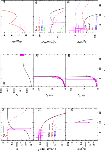
Figure 2: Comparison of analytical model predictions with observations for the best-fit model. The different panels indicate: (a) The volume-averaged neutral hydrogen fraction $x_{\rm HI}$, with observational lower limit from quasar absorption lines at $z=6$ and upper limit from Ly$\alpha$ emitters at $z=6.5$ (shown with arrows). In addition, the ionized fraction $x_{e}$ is shown by the dashed line. (b) SFR $\dot{\rho}_{*}$ for different stellar populations. (c) The number of source counts above a given redshift, with the observational upper limit from NICMOS HUDF shown by the arrow. The contribution to the source count is zero at low redshifts because of the J-dropout selection criterion. (d) Electron scattering optical depth, with observational constraint from WMAP 3-year data release. (e) Ly$\alpha$ effective optical depth. (f) Ly$\beta$ effective optical depth. (g) Evolution of Lyman-limit systems. (h) Photoionization rates for hydrogen, with estimates from numerical simulations (shown by points with error-bars; bhvs05 ). (i) Temperature of the mean density IGM.

The physics described above in the preceding sections can all be combined to construct a semi-analytical model for studying the thermal and ionization history of the IGM. We shall give an explicit example of one such model cf05 ; cf06b whose main features are: The model accounts for IGM inhomogeneities by adopting a lognormal distribution for $P(\Delta)$; reionization is said to be complete once all the low-density regions (say, with overdensities $\Delta<\Delta_{c}\sim 60$) are ionized. The ionization and thermal histories of neutral, HII and HeIII regions are followed simultaneously and self-consistently, treating the IGM as a multi-phase medium. Three types of reionization sources have been assumed: (i) metal-free (i.e. PopIII) stars having a Salpeter IMF in the mass range $1-100M_{\odot}$: they dominate the photoionization rate at high redshifts; (ii) PopII stars with sub-solar metallicities also having a Salpeter IMF in the mass range $1-100M_{\odot}$; (iii) quasars, which are significant sources of hard photons at $z\lesssim 6$; they have negligible effects on the IGM at higher redshifts.

As discussed earlier, reionization is accompanied by various feedback processes, which can affect subsequent star formation. In this model, radiative feedback is computed self-consistently from the evolution of the thermal properties of the IGM. Furthermore, the chemical feedback inducing the PopIII $\rightarrow$ PopII transition is implemented using a merger-tree “genetic” approach which determines the termination of PopIII star formation in a metal-enriched halo ssfc06 .

The predictions of the model are compared with a wide range of observational data sets, namely, (i) redshift evolution of Lyman-limit absorption systems ${\rm d}N_{\rm LLS}/{\rm d}z$ smih94 , (ii) the effective optical depths $\tau_{\rm eff}\equiv-\ln F$ for Ly$\alpha$ and Ly$\beta$ absorption in the IGM songaila04 , (iii) electron scattering optical depth $\tau_{\rm el}=\sigma_{T}c\int{\rm d}t~{}n_{e}$ (where $\sigma_{T}$ is the Thomson scattering cross section) as measured from CMBR experiments sbd++07 , (iv) temperature of the mean intergalactic gas stle99 , (v) cosmic star formation history $\dot{\rho}_{*}$ nchos04 , and (vi) source number counts at $z\approx 10$ from NICMOS HUDF bitf05 .

The data constrain the reionization scenario quite tightly. We find that hydrogen reionization starts at $z\approx 15$ driven by metal-free (PopIII) stars, and it is 90 per cent complete by $z\approx 8$. After a rapid initial phase, the growth of the volume filled by ionized regions slows down at $z\lesssim 10$ due to the combined action of chemical and radiative feedback, making reionization a considerably extended process completing only at $z\approx 6$. The number of photons per hydrogen at the end of reionization at $z\approx 6$ is only a few, which implies that reionization occurred in a “photon-starved” manner bh07 .

III.3 Clustering of sources

The formalism described till now works quite well for studying global properties of reionization. However, it is not adequate for studying the details of overlap of ionized regions in the pre-reionization epoch. The shapes and distribution of ionized regions are crucially dependent on the distribution of sources, in particular, their clustering and also on the density structure of the IGM. For example, if the sources are highly clustered, then it is expected that the overlap of the ionized bubble for nearby sources would be much earlier than what is expected from a random distribution of sources.

Modelling of reionization to such details have become important because of the 21cm observations which are likely to be available in near future. Before discussing the theoretical model, let us briefly outline the motivation behind 21cm experiments.

III.3.1 21cm observations

Perhaps the most promising prospect of detecting the fluctuations in the neutral hydrogen density during the (pre-)reionization era is through the 21 cm emission experiments fob06 , some of which are already taking data (GMRT , 21CMA ), and some are expected in future (MWA , LOFAR , SKA ). The basic principle which is central to these experiments is the neutral hydrogen hyperfine transition line at a rest wavelength of 21 cm. This line, when redshifted, is observable in radio frequencies ($\sim 150$ MHz for $z\sim 10$) as a brightness temperature:

$$\delta T_{b}(z,{\bf\hat{n}})=\frac{T_{S}-T_{\rm CMB}}{1+z}~{}\frac{3c^{3}\bar{A}_{10}n_{\rm HI}(z,{\bf\hat{n}})(1+z)^{3}}{16k_{\rm boltz}\nu_{0}^{2}T_{S}H(z)}$$ (50)

where $T_{S}$ is the spin temperature of the gas, $T_{\rm CMB}=2.76(1+z)~{}{\rm K}$ is the CMBR temperature, $A_{10}$ is the Einstein coefficient and $\nu_{0}=1420$ MHz is the rest frequency of the hyperfine line.

The observability of this brightness temperature against the CMBR background will depend on the relative values of $T_{S}$ and $T_{\rm CMB}$. Depending on which processes dominate at different epochs, $T_{S}$ will couple either to radiation ($T_{\rm CMB}$) or to matter (determined by the kinetic temperature $T_{k}$) pl08 . Almost in all models of reionization, the most interesting phase for observing the 21 cm radiation is $6\lesssim z\lesssim 20$. This is the phase where the IGM is suitably heated to temperatures much higher than CMBR (mostly due to X-ray heating cm04 ) thus making it observable in emission. In that case, we have $\delta T_{b}\propto n_{\rm HI}/n_{H}$, which means that the observations would directly probe the neutral hydrogen density in the Universe. Furthermore, this is the era when the bubble-overlapping phase is most active, and there is substantial neutral hydrogen to generate a strong enough signal. At low redshifts, after the IGM is reionized, $n_{\rm HI}$ falls by orders of magnitude and the 21 cm signal vanishes except in the high density neutral regions. Since the observations directly probe the neutral hydrogen density, one can use it to probe the detailed topology of the ionized regions in the pre-overlap phase. It is therefore essential to model the clustering of the sources accurately so as to predict the reionization topology.

III.3.2 Models of source clustering

There have been various approaches to account for the clustering of sources, most of them using the properties of the gaussian random field in terms of the extended Press-Schechter formalism. We have written equation (29) in terms of globally-averaged quantities; now let us write it in a slightly different form where the averaging is done over a spherical region of radius $R$ which has a density contrast $\delta$ (linearly extrapolated to present epoch). Then wl07 ; wm07 ; gw08

$$\frac{{\rm d}\langle Q_{\rm HII}\rangle_{\delta,R}}{{\rm d}t}=N_{\rm ion}\frac{{\rm d}\langle f_{\rm coll}\rangle_{\delta,R}}{{\rm d}t}-\langle Q_{\rm HII}\rangle_{\delta,R}~{}{\cal C}\alpha(T)n_{H}(1+\delta)$$ (51)

where we have assumed that reionization is primarily driven by galaxies and have used equation (48) to write $\dot{n}_{\rm ph}$ in terms of $\dot{f}_{\rm coll}$. The above equation can be solved for a given $\{\delta,R\}$ if we know the form of $\langle f_{\rm coll}\rangle_{\delta,R}$. It turns out that one has a simple generalization of equation (45) which encodes the clustering of sources at different scales and is given by bcek91

$$\langle f_{\rm coll}\rangle_{\delta,R}={\rm erfc}\left[\frac{\delta_{c}/D(t)-\delta}{\sqrt{2[\sigma^{2}(M_{\rm min})-\sigma^{2}(M)]}}\right]$$ (52)

where $M=4\pi R^{3}\bar{\rho}_{m}/3$ is the mass scale corresponding to $R$. The evolution of $\langle Q_{\rm HII}\rangle_{\delta,R}$ can be used for studying the filling fraction of ionized regions within the IGM on various scales $R$ as a function of overdensity $\delta$. In typical scenarios, this model predicts that reionization is driven by overlap of individual ionized regions around clustered sources residing in overdense regions of the Universe. This leads to an “inside-out” scenario of reionization where, on average, high-density regions are ionized first.

In a somewhat similar but slightly different approach, one can obtain the size distribution of the ionized regions at a given epoch. If we integrate equation (51) upto a certain time $t$, we can write the filling factor as

$$\langle Q_{\rm HII}\rangle_{\delta,R}=\frac{N_{\rm ion}\langle f_{\rm coll}\rangle_{\delta,R}}{1+N_{\rm rec}}$$ (53)

where $\langle Q_{\rm HII}\rangle_{\delta,R}~{}N_{\rm rec}=\int^{t}{\rm d}t^{\prime}~{}\langle Q_{\rm HII}\rangle_{\delta,R}~{}{\cal C}~{}\alpha(T)n_{H}(1+\delta)$ is the number of recombinations within the region over the history of the IGM. Hence, the condition for the region to be fully ionized $\langle Q_{\rm HII}\rangle_{\delta,R}\geq 1$ is given by a condition on the collapsed faction fzh04b ; mf07 ; mlz+07

$$\langle f_{\rm coll}\rangle_{\delta,R}\geq N_{\rm ion}^{-1}(1+N_{\rm rec})$$ (54)

The condition for a region to be “self-ionized” can be converted into a condition in terms of the density contrast $\delta$. The problem then is very similar to the problem of collapse of haloes where it is studied whether the density averaged over a spherical volume exceeds a critical value (“barrier”) st02 . The only difference here is that the barrier is much complex than the collapse of halo problem. One can approximate the barrier with a linear one and then write a distribution of sizes similar to equation (38). The results obtained from this approach is very similar to the one obtained from the previous one that reionization at large scales proceeds in a “inside-out” fashion.

Both the approaches described above have also been extended to simulation boxes and used for making mock maps of the neutral hydrogen distribution which is extremely useful for 21cm observations. These methods essentially give a semi-analytic (or semi-numeric) approach to deal with the radiative transfer problem and can be used for making maps using much less computing power.

III.3.3 Recombination and self-shielding

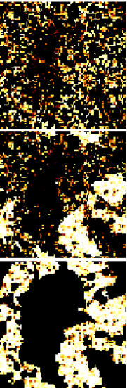
Figure 3: Ionization maps for a IGM with ionized hydrogen fraction of 75% for models with different assumptions regarding the spatial distribution of sinks and sources of ionizing radiation chr09 . The black regions represent ionized ones. The left panel considers only homogenous recombination while the middle and right panels consider different levels of self-shielding. The thickness of the slice shown is 1$h^{-1}$Mpc.

In the above approaches, recombinations in the IGM an be accounted for only by averaging over a spherical region. In reality, even if a given spherical region contains enough photons to self-ionize, the high-density clumps within the region will remain neutral for a longer period because of their high recombination rate and thus alter the nature of the ionization field. A simple prescription to describe the presence of such neutral clumps by assuming that regions with overdensities above a critical value ($\Delta>\Delta_{c}$) remain neutral as we discussed earlier. Unfortunately this is also not fully appropriate as many of the high-density regions are expected to harbour ionizing sources. Whether a region remains neutral will depend on two competing factors, the local density (which determines the recombination rate) and the proximity to ionizing sources (which determines the number of photons available). It is thus important to include a realistic spatial distribution of recombinations into the formalisms for making ionization maps.

A possible way of modelling the recombinations in high-density regions is to use a self-shielding criterion. In order to be ionized, a given point should satisfy the condition that it cannot remain self-shielded, i.e., it should not be a Lyman-limit system. In terms of the column density of the system, the condition can be written as chr09

$$N_{\rm HI}\equiv n_{\rm HI}({\bf x})L({\bf x})\sigma_{\rm HI}\leq 1,$$ (55)

where $n_{\rm HI}({\bf x})$ is the number density of neutral hydrogen at the given point and $L({\bf x})$ is the size of the of the absorber. It turns out that the topology of reionization is very different if such self-shielding is taken into account particularly when reionization is extended and photon-starved as can be seen from Figure 3. Initially reionization proceeds inside-out with the high density regions hosting the sources of ionizing sources becoming ionized first. In the later stages, the high density regions which are far from sources remain neutral and reionization proceeds deep into the underdense regions before slowly evaporating denser regions. Such models can, in principle, be constrained by the first generation of 21 cm experiments.

IV Current status and Future

In this section, let us review the current status of various approaches to studying reionization and their future prospects.

IV.1 Simulations

Though the analytical studies mentioned above allow us to develop a good understanding of the different processes involved in reionization, they can take into account the physical processes only in some approximate sense. In fact, a detailed and complete description of reionization would require locating the ionizing sources, resolving the inhomogeneities in the IGM, following the scattering processes through detailed radiative transfer, and so on. Numerical simulations, in spite of their limitations, have been of immense importance in these areas.

Since the ionizing photons during early stages of reionization mostly originate from smaller haloes which are far more numerous than the larger galaxies at high redshifts. The need to resolve such small structures requires the simulation boxes to have high enough resolution. On the other hand, these ionizing sources were strongly clustered at high redshifts and, as a consequence, the ionized regions they created are expected to overlap and grow to very large sizes, reaching upto tens of Mpc bl04 ; fo05 ; cen05 . As already discussed, the many orders of magnitude difference between these length scales demand extremely high computing power from any simulations designed to study early structure formation from the point of view of reionization.

To simulate reionization, one usually runs a N-body simulation (either dark matter only or including baryons) to generate the large-scale density field, identifies haloes within the density field and assign ionizing photons to the haloes using a assumption like equation (48). It turns out that the most difficult step is to solve the radiative transfer equation and study the growth of ionized regions. In principle, one could solve equation (4) directly for the intensity at every point in the seven-dimensional $(t,{\bf x},{\bf n},\nu)$ space, given the absorption coefficient and the emissivity. However, the high dimensionality of the problem makes the solution of the complete radiative transfer equation well beyond our capabilities, particularly since we do not have any obvious symmetries in the problem and often need high spatial and angular resolution in cosmological simulations. Hence, the approach to the problem has been to use different numerical schemes and approximations, like ray-tracing anm99 ; rs99 ; sah01 ; cen02 ; rnas02 ; sir04 ; bmw04 ; isr05 ; impmsa06 , Monte Carlo methods cfmr01 ; mfc03 ; mck09 , local depth approximation go97 and others ps08 . At present, most of the simulations do not have enough resolution to reliably identify the low mass $\sim 10^{8}M_{\odot}$ sources which were probably responsible for early stages of reionization. Also, there are difficulties in resolving the small scale structures which contribute significantly to the clumpiness in the IGM and hence extend the reionization process.

IV.2 Various observational probes

Finally, we review certain observations which shape our understanding of reionization.

IV.2.1 Absorption spectra of high redshift sources

We have already discussed that the primary evidence for reionization comes from absorption spectra of quasars (Ly$\alpha$ forest) at $z<6$. We have also discussed that the effective optical depth of Ly$\alpha$ photons becomes significantly large at $z\gtrsim 6$ implying regions with high transmission in the Ly$\alpha$ forest becoming rare at high redshifts fsb++06 ; wdr++09 . Therefore the standard methods of analyzing the Ly$\alpha$ forest (like the probability distribution function and power spectrum) are not very effective. Amongst alternate methods, one can use the the distribution of dark gaps croft98 ; sc02 which are defined as contiguous regions of the spectrum having an optical depth above a threshold value sc02 ; fsb++06 . It has been found that the current observations constrain the neutral hydrogen fraction $x_{\rm HI}<0.36$ at $z=6.3$ gffc08 . It is expected that the SDSS and Palomar-Quest survey ldc++05 would detect $\sim 30$ quasars at these redshifts within the next few years and hence we expect robust conclusions from such studies in very near future.

Like quasars, one can also use absorption spectra of other high redshift energetic sources like gamma ray bursts (GRBs) and supernovae. In fact, analyses using the damping wing effects of the Voigt profile have been already performed on the GRB detected at a redshift $z=6.3$, and the wing shape is well-fit by a neutral fraction $x_{\rm HI}<0.17$ tkk++06 . The dark gap width distribution gives a similar constraint $x_{\rm HI}=(6.4\pm 0.3)\times 10^{-5}$ gsfc08 . In order to obtain more stringent limits on reionization, it is important to increase the sample size of $z>6$ GRBs.

In addition to hydrogen reionization, the Ly$\alpha$ forest in the quasar absorption lines at $z\approx 3$ can also be used for studying reionization of singly ionized helium to doubly ionized state (the reionization of neutral helium to singly ionized state follows hydrogen for almost all types of sources). The helium reionization coincides with the rise in quasar population at $z\sim 3$ and it effects the thermal history of the IGM at these redshifts. However, there are various aspects of the observation that are not well understood and requires much detailed modelling of helium reionization gnbos05 ; bvkhc08 ; fo08 ; bof08 ; mlz+09 .

IV.2.2 CMBR observations

As we have discussed already, the first evidence for an early reionization epoch came from the CMBR polarization data. This data is going to be much more precise in future with experiments like PLANCK, and is expected to improve the constraints on $\tau_{\rm el}$. With improved statistical errors, it might be possible to distinguish between different evolutions of the ionized fraction, particularly with E-mode polarization auto-correlation, as is found from theoretical calculations hhkk03 ; bpsscf08 . An alternative option to probe reionization through CMBR is through the small scale observations of temperature anisotropies. It has been well known that the scattering of the CMBR photons by the bulk motion of the electrons in clusters gives rise to a signal at large multipoles $\ell\sim 1000$, known as the kinetic Sunyaev Zeldovich (SZ) effect. Such a signal can also originate from the fluctuations in the distribution of free electrons arising from cosmic reionization. It turns out that for reionization, the signal is dominated by the patchiness in the $n_{e}$-distribution. Now, in most scenarios of reionization, it is expected that the distribution of neutral hydrogen would be quite patchy in the pre-overlap era, with the ionized hydrogen mostly contained within isolated bubbles. The amplitude of this signal is significant around $\ell\sim 1000$ and is usually comparable to or greater than the signal arising from standard kinetic SZ effect. Theoretical estimates of the signal have been performed for various reionization scenarios, and it has been predicted that the experiment can be used for constraining reionization history schkm03 ; mfhzz05 . Also, it is possible to have an idea about the nature of reionization sources, as the signal from UV sources, X-ray sources and decaying particles are quite different. With multi-frequency experiments like Atacama Cosmology Telescope (ACT) and South Pole Telescope (SPT) coming up in near future, this promises to put strong constraints on the reionization scenarios.

IV.2.3 Ly$\alpha$ emitters

In recent years, a number of groups have studied star-forming galaxies at $z\sim 6-7$, and measurements of the Ly$\alpha$ emission line luminosity function evolution provide another useful observational constraint mr04 ; sye++05 . While the quasar absorption spectra probe the neutral hydrogen fraction regime $x_{\rm HI}\leq 0.01$, this method is sensitive to the range $x_{\rm HI}\sim 0.1-1.0$. Ly$\alpha$ emission from galaxies is expected to be suppressed at redshifts beyond reionization because of the absorption due to neutral hydrogen, which clearly affects the evolution of the luminosity function of such Ly$\alpha$ emitters at high redshifts hc05 ; mr04 ; fhz04 . Thus a comparison of the luminosity functions at different redshifts could be used for constraining the reionization. Through a simple analysis, it was found that the luminosity functions at $z=5.7$ and $z=6.5$ are statistically consistent with one another thus implying that reionization was largely complete at $z\approx 6.5$. More sophisticated calculations on the evolution of the luminosity function of Ly$\alpha$ emitters mr04 ; fzh06 ; hc05 suggest that the neutral fraction of hydrogen at $z=6.5$ should be less than 50 per cent mr06 . Unfortunately, the analysis of the Ly$\alpha$ emitters at high redshifts is complicated by various factors like the velocity of the sources with respect to the surrounding IGM, the density distribution and the size of ionized regions around the sources and the clustering of sources. It is thus extremely important to have detailed models of Ly$\alpha$ emitting galaxies in order to use them for constraining reionization.

IV.2.4 Sources of reionization

As we discussed earlier, a major challenge in our understanding of reionization depends on our knowledge of the sources, particularly at high redshifts. As we understand at present, neither the bright $z>6$ quasars discovered by the SDSS group fsr++05 nor the faint ones detected in X-ray observations bcc++03 produce enough photons to reionize the IGM. The discovery of star-forming galaxies at $z>6.5$ hcm++02 ; ktk++03 ; kesr04 has resulted in speculation that early galaxies produce bulk of the ionizing photons for reionization. Unfortunately, there are significant uncertainties in constraining the amount of ionizing radiation at these redshifts because the bulk of ionizing photons could be produced by faint sources which are beyond the present sensitivities. In fact, some models have predicted that the $z>7$ sources identified in these surveys are relatively massive $(M\approx 10^{9}M_{\odot}$) and rare objects which are only marginally ($\approx 1\%$) contributing to the reionization photon budget cf07 . A much better prospect of detecting these sources would be through the Ultra-Deep Imaging Survey using the future telescope JWST.

IV.2.5 21cm experiments

We have already discussed the basic theory behind detecting the fluctuations in the neutral hydrogen density through the 21 cm emission experiments. There are essentially two complementary approaches to studying reionization using 21 cm signal. The first one is through global statistical properties of the neutral hydrogen signal, like the power spectrum mh04b ; zfh04 ; abp05 ; ba04 ; sethi05 ; dcb07 . The second one is to directly detect the ionized bubbles around sources, either through blind surveys or via targetted observations wlb05 ; aa07 ; gw08 ; mgfc07 ; dbc07 ; dmbc08 .

The major difficulty in obtaining the cosmological signal from these experiments is that it is expected to be only a small contribution buried deep in the emission from other astrophysical sources (foregrounds) and in the system noise swmd99 ; dpar02 ; om03 ; cf04 ; sck05 ; gnb08 ; abc08 . It is thus a big challenge to detect the signal which is of cosmological importance from the other contributions that are orders of magnitude larger. Once such challenges are dealt with, this probe will be the strongest probe for not only reionization, but of the matter distribution at very small scales during the dark ages.

V Concluding remarks

We have discussed the analytical approaches to model different aspects of reionization which will help in understanding the most relevant physical processes. In an explicit example, we have shown how to apply this formalism for constraining the reionization history using a variety of observational data. These constraints imply that reionization is an extended process over a redshift range $15>z>6$. It is most likely driven by the first sources which form in small mass haloes. However, there are still uncertainties about the exact nature of these sources and the detailed topology of ionized regions. Such details are going to be addressed in near future as new observations, both space-borne and ground-based, are likely to settle these long-standing questions. From the theoretical point of view, it is thereby important to develop detailed analytical and numerical models to extract the maximum information about the physical processes relevant for reionization out of the expected large and complex data sets.

References

- (1) J. Dunkley et al., ApJS 180, 306 (2009).
- (2) A. Loeb and R. Barkana, ARA&A 39, 19 (2001).
- (3) R. Barkana and A. Loeb, Phys. Rep. 349, 125 (2001).
- (4) T. R. Choudhury and A. Ferrara, in Cosmic Polarization, edited by R. Fabbri (Research Signpost, India, 2006), p. 205.
- (5) X. Fan, C. L. Carilli, and B. Keating, ARA&A 44, 415 (2006).
- (6) P. J. E. Peebles, Principles of physical cosmology (Princeton, NJ: Princeton University Press, USA, 1993).
- (7) H. M. P. Couchman and M. J. Rees, MNRAS 221, 53 (1986).
- (8) J. A. Peacock, Cosmological Physics (Cambridge, UK: Cambridge University Press, UK, 1999).
- (9) T. Padmanabhan, Theoretical Astrophysics, Volume III: Galaxies and Cosmology (Cambridge, England: Cambridge University Press, UK, 2002).
- (10) J. S. B. Wyithe and A. Loeb, ApJ 586, 693 (2003).
- (11) N. Y. Gnedin, ApJ 535, 530 (2000).
- (12) T. R. Choudhury and A. Ferrara, MNRAS 371, L55 (2006).
- (13) T. Abel, M. L. Norman, and P. Madau, ApJ 523, 66 (1999).
- (14) F. Haardt and P. Madau, ApJ 461, 20 (1996).
- (15) P. Madau, F. Haardt, and M. J. Rees, ApJ 514, 648 (1999).
- (16) J. Miralda-Escudé, M. Haehnelt, and M. J. Rees, ApJ 530, 1 (2000).
- (17) H. G. Bi, G. Boerner, and Y. Chu, A&A 266, 1 (1992).
- (18) H. Bi, ApJ 405, 479 (1993).
- (19) N. Y. Gnedin and L. Hui, ApJ 472, L73 (1996).
- (20) H. Bi and A. F. Davidsen, ApJ 479, 523 (1997).
- (21) L. Hui, N. Y. Gnedin, and Y. Zhang, ApJ 486, 599 (1997).
- (22) N. Y. Gnedin and L. Hui, MNRAS 296, 44 (1998).
- (23) T. R. Choudhury, T. Padmanabhan, and R. Srianand, MNRAS 322, 561 (2001).
- (24) T. R. Choudhury, R. Srianand, and T. Padmanabhan, ApJ 559, 29 (2001).
- (25) R. Cen, J. Miralda-Escudé, J. P. Ostriker, and M. Rauch, ApJ 437, L9 (1994).
- (26) Y. Zhang, P. Anninos, and M. L. Norman, ApJ 453, L57 (1995).
- (27) L. Hernquist, N. Katz, D. H. Weinberg, and J. Miralda-Escudé, ApJ 457, L51 (1996).
- (28) J. Miralda-Escudé, R. Cen, J. P. Ostriker, and M. Rauch, ApJ 471, 582 (1996).
- (29) M. Viel et al., MNRAS 336, 685 (2002).
- (30) P. McDonald et al., ApJ 635, 761 (2005).
- (31) J. S. Bolton, M. G. Haehnelt, M. Viel, and V. Springel, MNRAS 357, 1178 (2005).
- (32) P. McDonald et al., ApJS 163, 80 (2006).
- (33) J. S. Bolton et al., MNRAS 386, 1131 (2008).
- (34) A. Songaila, AJ 127, 2598 (2004).
- (35) X. Fan et al., AJ 132, 117 (2006).
- (36) M. Rauch, ARA&A 36, 267 (1998).
- (37) J. E. Gunn and B. A. Peterson, ApJ 142, 1633 (1965).
- (38) C. J. Willott et al., AJ 137, 3541 (2009).
- (39) F. Paresce, C. F. McKee, and S. Bowyer, ApJ 240, 387 (1980).
- (40) M. Schirber and J. S. Bullock, ApJ 584, 110 (2003).
- (41) J. Miralda-Escudé, ApJ 597, 66 (2003).
- (42) P. Petitjean, J. Bergeron, R. F. Carswell, and J. L. Puget, MNRAS 260, 67 (1993).
- (43) L. J. Storrie-Lombardi, R. G. McMahon, and M. J. Irwin, MNRAS 283, L79 (1996).
- (44) W. A. Chiu and J. P. Ostriker, ApJ 534, 507 (2000).
- (45) W. A. Chiu, X. Fan, and J. P. Ostriker, ApJ 599, 759 (2003).
- (46) T. R. Choudhury and A. Ferrara, MNRAS 361, 577 (2005).
- (47) W. H. Press and P. Schechter, ApJ 187, 425 (1974).
- (48) S. Sasaki, PASJ 46, 427 (1994).
- (49) Z. Haiman, T. Abel, and M. J. Rees, ApJ 534, 11 (2000).
- (50) M. Ricotti, N. Y. Gnedin, and J. M. Shull, ApJ 560, 580 (2001).
- (51) S. C. O. Glover and P. W. J. L. Brand, MNRAS 321, 385 (2001).
- (52) R. S. Somerville and J. R. Primack, MNRAS 310, 1087 (1999).
- (53) S. Samui, R. Srianand, and K. Subramanian, MNRAS 377, 285 (2007).
- (54) C. Leitherer et al., ApJS 123, 3 (1999).
- (55) G. Bruzual and S. Charlot, MNRAS 344, 1000 (2003).
- (56) V. Bromm, R. P. Kudritzki, and A. Loeb, ApJ 552, 464 (2001).
- (57) D. Schaerer, A&A 382, 28 (2002).
- (58) M. Ricotti and J. M. Shull, ApJ 542, 548 (2000).
- (59) K. Wood and A. Loeb, ApJ 545, 86 (2000).
- (60) N. Y. Gnedin, A. V. Kravtsov, and H.-W. Chen, ApJ 672, 765 (2008).
- (61) J. H. Wise and R. Cen, ApJ 693, 984 (2009).
- (62) C. C. Steidel, M. Pettini, and K. L. Adelberger, ApJ 546, 665 (2001).
- (63) A. E. Shapley et al., ApJ 651, 688 (2006).
- (64) A. K. Inoue, I. Iwata, and J.-M. Deharveng, MNRAS 371, L1 (2006).
- (65) H.-W. Chen, J. X. Prochaska, and N. Y. Gnedin, ApJ 667, L125 (2007).
- (66) J. S. B. Wyithe and A. Loeb, MNRAS 375, 1034 (2007).
- (67) B. Ciardi and A. Ferrara, Space Sci. Rev. 116, 625 (2005).
- (68) G. T. Richards et al., AJ 131, 2766 (2006).
- (69) P. Madau et al., ApJ 604, 484 (2004).
- (70) R. Schneider, R. Salvaterra, A. Ferrara, and B. Ciardi, MNRAS 369, 825 (2006).
- (71) L. J. Storrie-Lombardi, R. G. McMahon, M. J. Irwin, and C. Hazard, ApJ 427, L13 (1994).
- (72) D. N. Spergel et al., ApJS 170, 377 (2007).
- (73) J. Schaye, T. Theuns, A. Leonard, and G. Efstathiou, MNRAS 310, 57 (1999).
- (74) K. Nagamine et al., ApJ 610, 45 (2004).
- (75) R. J. Bouwens, G. D. Illingworth, R. I. Thompson, and M. Franx, ApJ 624, L5 (2005).
- (76) J. S. Bolton and M. G. Haehnelt, MNRAS 382, 325 (2007).
- (77) S. R. Furlanetto, S. P. Oh, and F. H. Briggs, Phys. Rep. 433, 181 (2006).
- (78) J. R. Pritchard and A. Loeb, Phys. Rev. D 78, 103511 (2008).
- (79) X. Chen and J. Miralda-Escudé, ApJ 602, 1 (2004).
- (80) J. S. B. Wyithe and M. F. Morales, MNRAS 379, 1647 (2007).
- (81) P. M. Geil and J. S. B. Wyithe, MNRAS 386, 1683 (2008).
- (82) J. R. Bond, S. Cole, G. Efstathiou, and N. Kaiser, ApJ 379, 440 (1991).
- (83) S. R. Furlanetto, M. Zaldarriaga, and L. Hernquist, ApJ 613, 1 (2004).
- (84) A. Mesinger and S. Furlanetto, ApJ 669, 663 (2007).
- (85) M. McQuinn et al., MNRAS 377, 1043 (2007).
- (86) R. K. Sheth and G. Tormen, MNRAS 329, 61 (2002).
- (87) T. R. Choudhury, M. G. Haehnelt, and J. Regan, MNRAS 394, 960 (2009).
- (88) S. R. Furlanetto and S. P. Oh, MNRAS 363, 1031 (2005).
- (89) R. Barkana and A. Loeb, ApJ 609, 474 (2004).
- (90) R. Cen, Preprint: astro-ph/0507014, 2005.
- (91) A. O. Razoumov and D. Scott, MNRAS 309, 287 (1999).
- (92) A. Sokasian, T. Abel, and L. E. Hernquist, New Astron. 6, 359 (2001).
- (93) R. Cen, ApJS 141, 211 (2002).
- (94) A. O. Razoumov, M. L. Norman, T. Abel, and D. Scott, ApJ 572, 695 (2002).
- (95) P. R. Shapiro, I. T. Iliev, and A. C. Raga, MNRAS 348, 753 (2004).
- (96) I. T. Iliev, P. R. Shapiro, and A. C. Raga, MNRAS 361, 405 (2005).
- (97) J. Bolton, A. Meiksin, and M. White, MNRAS 348, L43 (2004).
- (98) I. T. Iliev et al., MNRAS 369, 1625 (2006).
- (99) B. Ciardi, A. Ferrara, S. Marri, and G. Raimondo, MNRAS 324, 381 (2001).
- (100) A. Maselli, A. Ferrara, and B. Ciardi, MNRAS 345, 379 (2003).
- (101) A. Maselli, B. Ciardi, and A. Kanekar, MNRAS 393, 171 (2009).
- (102) N. Y. Gnedin and J. P. Ostriker, ApJ 486, 581 (1997).
- (103) A. H. Pawlik and J. Schaye, MNRAS 389, 651 (2008).
- (104) R. A. C. Croft, in Olinto A. V., Frieman J. A., Schramm D. N. ed., Eighteenth Texas Symposium on Relativistic Astrophysics. (World Scientific, River Edge, N. J., 1998), pp. 664–+.
- (105) A. Songaila and L. L. Cowie, AJ 123, 2183 (2002).
- (106) S. Gallerani, A. Ferrara, X. Fan, and T. R. Choudhury, MNRAS 386, 359 (2008).
- (107) O. López-Cruz et al., in Revista Mexicana de Astronomia y Astrofisica Conference Series, edited by A. M. Hidalgo-Gámez, J. J. González, J. M. Rodríguez Espinosa, and S. Torres-Peimbert (Instituto de Astronomía, Universidad Nacional Autónoma de México, Mexico, 2005), pp. 164–169.
- (108) T. Totani et al., PASJ 58, 485 (2006).
- (109) S. Gallerani, R. Salvaterra, A. Ferrara, and T. R. Choudhury, MNRAS 388, L84 (2008).
- (110) L. Gleser et al., MNRAS 361, 1399 (2005).
- (111) S. R. Furlanetto and S. P. Oh, ApJ 682, 14 (2008).
- (112) J. S. Bolton, S. P. Oh, and S. R. Furlanetto, ArXiv e-prints (2008).
- (113) M. McQuinn et al., ApJ 694, 842 (2009).
- (114) G. P. Holder, Z. Haiman, M. Kaplinghat, and L. Knox, ApJ 595, 13 (2003).
- (115) C. Burigana et al., MNRAS 385, 404 (2008).
- (116) M. G. Santos et al., ApJ 598, 756 (2003).
- (117) M. McQuinn et al., ApJ 630, 643 (2005).
- (118) S. Malhotra and J. E. Rhoads, ApJ 617, L5 (2004).
- (119) D. Stern et al., ApJ 619, 12 (2005).
- (120) Z. Haiman and R. Cen, ApJ 623, 627 (2005).
- (121) S. R. Furlanetto, L. Hernquist, and M. Zaldarriaga, MNRAS 354, 695 (2004).
- (122) S. R. Furlanetto, M. Zaldarriaga, and L. Hernquist, MNRAS 365, 1012 (2006).
- (123) S. Malhotra and J. E. Rhoads, ApJ 647, L95 (2006).
- (124) X. Fan et al., Preprint: astro-ph/0512080, 2005.
- (125) A. J. Barger et al., ApJ 584, L61 (2003).
- (126) E. M. Hu et al., ApJ 568, L75 (2002).
- (127) K. Kodaira et al., PASJ 55, L17 (2003).
- (128) J.-P. Kneib, R. S. Ellis, M. R. Santos, and J. Richard, ApJ 607, 697 (2004).
- (129) T. R. Choudhury and A. Ferrara, MNRAS 380, L6 (2007).
- (130) M. F. Morales and J. Hewitt, ApJ 615, 7 (2004).
- (131) Z.-H. Zhu, M.-K. Fujimoto, and X.-T. He, A&A 417, 833 (2004).
- (132) S. S. Ali, S. Bharadwaj, and B. Pandey, MNRAS 363, 251 (2005).
- (133) S. K. Sethi, MNRAS 363, 818 (2005).
- (134) K. K. Datta, T. R. Choudhury, and S. Bharadwaj, MNRAS 378, 119 (2007).
- (135) S. Bharadwaj and S. S. Ali, MNRAS 352, 142 (2004).
- (136) J. S. B. Wyithe, A. Loeb, and D. G. Barnes, ApJ 634, 715 (2005).
- (137) M. A. Alvarez and T. Abel, MNRAS 380, L30 (2007).
- (138) A. Maselli, S. Gallerani, A. Ferrara, and T. R. Choudhury, MNRAS 376, L34 (2007).
- (139) K. K. Datta, S. Bharadwaj, and T. R. Choudhury, MNRAS 382, 809 (2007).
- (140) K. K. Datta, S. Majumdar, S. Bharadwaj, and T. R. Choudhury, MNRAS 391, 1900 (2008).
- (141) P. A. Shaver, R. A. Windhorst, P. Madau, and A. G. de Bruyn, A&A 345, 380 (1999).
- (142) T. Di Matteo, R. Perna, T. Abel, and M. J. Rees, ApJ 564, 576 (2002).
- (143) S. P. Oh and K. J. Mack, MNRAS 346, 871 (2003).
- (144) A. Cooray and S. R. Furlanetto, ApJ 606, L5 (2004).
- (145) M. G. Santos, A. Cooray, and L. Knox, ApJ 625, 575 (2005).
- (146) S. S. Ali, S. Bharadwaj, and J. N. Chengalur, MNRAS 385, 2166 (2008).
- (147) L. Gleser, A. Nusser, and A. J. Benson, MNRAS 391, 383 (2008).