Global Sensitivity Analysis of Biochemical Reaction Networks via Semidefinite Programming

Abstract

We study the problem of computing outer bounds for the region of steady states of biochemical reaction networks modelled by ordinary differential equations, with respect to parameters that are allowed to vary within a predefined region. Using a relaxed version of the corresponding feasibility problem and its Lagrangian dual, we show how to compute certificates for regions in state space not containing any steady states. Based on these results, we develop an algorithm to compute outer bounds for the region of all feasible steady states. We apply our algorithm to the sensitivity analysis of a Goldbeter–Koshland enzymatic cycle, which is a frequent motif in reaction networks for regulation of metabolism and signal transduction. Copyright © 2008 IFAC.

1 Introduction

A basic question in the analysis of biochemical reaction networks is how steady state concentrations change with parameters. Metabolic Control Analysis (MCA) is a classical tool to answer this question [Kacser et al., 1995], where the analysis is based on a linear approximation of the system’s equations around the steady state. Due to the linear approximation, results from MCA are only valid if parameter variations are small. However, in natural biochemical reaction networks, one usually faces large parameter variations: in genetic engineering, common techniques like gene knock-outs or knock-downs, overexpression or binding site mutations typically give rise to large parameter variations.

It follows that there is a need to compute changes in steady state values which are due to large parameter variations. One approach to broaden the validity of results from MCA to larger parameter variations is to include higher order approximations at the nominal point [Streif et al., 2007]. Although such an approach may extend the validity of the approximation, it still gives results which are in general only locally valid.

We will thus rather take a different route and study the problem from the perspective of computing the set of all steady states for given ranges in which parameter values may vary. In contrast to classical, local sensitivity analysis, such an approach allows to directly evaluate the range that steady state concentrations can take for given parameter ranges. The drawback is that it is not directly possible to assess the influence of individual parameters on the steady state. However, by repeating the computation for different parameter ranges, also this information may be obtained.

Computing the set of steady states analytically is only possible in very rare cases. Even if an analytical solution for the steady state is known, computing the corresponding set for all possible parameter values may be difficult. Due to this difficulty, non-deterministic approaches are frequently used to solve this problem. A common tool for this kind of analysis are Monte Carlo methods [Robert and Casella, 2004], which are routinely applied in the analysis of uncertain biochemical reaction networks [Alves and Savageau, 2000, Feng et al., 2004]. However, Monte Carlo methods do not give reliable results in the sense that it is possible to miss important solutions, which is particularly problematic for highly nonlinear dependencies of the steady state on parameters. Also, Monte Carlo approaches to the problem at hand typically require that all of the possibly multiple steady states for specific parameter values can be computed explicitly, which is often a difficult task in itself.

Continuation methods that track the changes in steady state values upon parameter variations are an efficient computational tool for this problem [Richter and DeCarlo, 1983, Kuznetsov, 1995], but are restricted to low-dimensional parameter variations and are thus in general unsuitable for exploring higher-dimensional parameter spaces.

Global optimization methods employing branch and bound techniques or interval arithmetics would in principle be suited to compute steady state regions [Maranas and Floudas, 1995, Neumaier, 1990]. However, it seems that the corresponding computational cost has obstructed their application to the analysis of biochemical reaction networks so far.

In this paper, we propose a new approach to obtain reliable bounds on steady state values under uncertain parameters in a computationally efficient way. The paper is structured as follows. In Section 3, we study the problem of finding certificates that a given set in state space does not contain a steady state for any parameters in a given set in parameter space. In Section 4, we use the results obtained in Section 3 to develop an algorithm that computes outer bounding regions of steady state values for a given set in which parameters vary. The application of the proposed analysis method is shown for two example reaction networks in Section 5.

Mathematical notation

The space of real symmetric $n\times n$ matrices is denoted as $\mathcal{S}^{n}$. The order operator with respect to the positive orthant in $\mathbb{R}^{m\times n}$ is denoted as “$\boldsymbol{\leq}$”, i.e. $0\boldsymbol{\leq}X\in\mathbb{R}^{m\times n}\Leftrightarrow 0\leq X_{i,j}$ for $i=1,\dotsc,m$, $j=1,\dotsc,n$. The order operator with respect to the cone of positive semidefinite (PSD) matrices in $\mathcal{S}^{n}$ is denoted as “$\preccurlyeq$”, i.e. $0\preccurlyeq X\in\mathcal{S}^{n}\Leftrightarrow X$ is PSD. The trace of a quadratic matrix $X\in\mathbb{R}^{n\times n}$ is denoted as $\mathrm{\mathop{tr}}X$.

2 Problem statement and basic idea

We consider biochemical reaction networks that are modelled by ordinary differential equations. This modelling framework is quite general and covers most metabolic networks as well as many signal transduction pathways, if spatial effects can be neglected. Mathematically, such models are commonly written as

$$\dot{x}=Sv(x,p),$$ (1)

where $x\in\mathbb{R}^{n}$ is the concentration vector, $S\in\mathbb{R}^{n\times m}$ is the stoichiometric matrix, $p\in\mathbb{R}^{m}$ is the vector of parameter values and $v(x,p)\in\mathbb{R}^{m}$ is the vector of reaction fluxes [Klipp et al., 2005]. Throughout this paper, we assume that fluxes are modelled using the law of mass action, where $v$ takes the form

$$v_{j}(x,p)=p_{j}\prod_{k=1}^{n}x_{k}^{\sigma_{jk}},$$ (2)

for $j=1,\dotsc,m$. The constants $\sigma_{jk}$ are integers representing the stoichiometric coefficient of the species $k$ taking part in the $j$-th reacting complex. In the case of mass action kinetics, the dimensions of the parameter vector and the flux vector are in general the same. Note that our results can be extended to rational functions describing the fluxes, such as used for Michaelis–Menten kinetics, in a straightforward way.

The problem under consideration can be formulated as follows. Given a set $\mathcal{P}\subset\mathbb{R}^{m}$ in parameter space, compute a set $\mathcal{X}_{s}\subset\mathbb{R}^{n}$ that contains all steady states of the system (1) for parameter values taken from $\mathcal{P}$. Ideally, the set $\mathcal{X}_{s}$ should be as small as possible, such that for all $x_{s}\in\mathcal{X}_{s}$, there is a parameter vector $p\in\mathcal{P}$ with $Sv(x_{s},p)=0$. Then,

$$\mathcal{X}_{s}=\left\{x\in\mathbb{R}^{m}\mid\exists p\in\mathcal{P}:Sv(x,p)=0\right\}.$$ (3)

However, for the case $m>1$, when continuation methods are not suitable, there are at present no general methods to compute $\mathcal{X}_{s}$ efficiently and reliably.

We present a method to address this problem that works for arbitrarily large state and parameter spaces, does not need to compute steady state values explicitly and is computationally efficient. The method is able to compute reliable, though conservative outer bounds on the set $\mathcal{X}_{s}$ of all steady states.

In order to search for sets of steady states for a given parameter set $\mathcal{P}$, we need means to test whether a candidate solution $\mathcal{X}_{s}$ obtained in such a search is actually valid or not. Such a test is readily formulated as a feasibility problem. Moreover, we will see that the Lagrangian dual for this feasibility problem allows to certify given regions in state space as not containing a steady state for any parameter value from the set $\mathcal{P}$. We then develop an algorithm that uses this information to construct outer bounds on the region $\mathcal{X}_{s}$ of all steady states.

In this paper, we consider only hyperrectangles for the sets $\mathcal{X}_{s}$ and $\mathcal{P}$ in state and parameter space. An extension to more general convex polytopes is in principle easy from the theoretical perspective, but it requires a much more elaborate implementation on the practical side.

3 Feasibility of steady state regions

3.1 Feasibility problem and semidefinite relaxation

The problem of testing whether a given hyperrectangle $\mathcal{X}_{s}$ in state space contains steady states of the system (1), for some parameter values in a given hyperrectangle $\mathcal{P}$ in parameter space, can be formulated as the following feasibility problem:

$$\textnormal{(}P):\ \left\{\ \begin{aligned} \textnormal{find}&&x\in\mathbb{R}^{n},&\ p\in\mathbb{R}^{m}&&\\ \textnormal{s.t.}&&Sv(x,p)&=0&\\ &&p_{j,min}\leq p_{j}&\leq p_{j,max}&&j=1,\dotsc,m\\ &&x_{i,min}\leq x_{i}&\leq x_{i,max}&&i=1,\dotsc,n.\end{aligned}\right.$$ (4)

The same problem appears in the context of parameter identification in a recent paper by Kuepfer et al. [2007]. They developped a method that uses an infeasibility certificate for the problem (4) to exclude regions in parameter space from the identification procedure, given a set of steady state measurements. In this section, we take their approach to find an infeasibility certificate for problem (4), but give more details about the underlying mathematical techniques.

Relaxing the feasiblity problem (4) to a semidefinite program [Vandenberghe and Boyd, 1996] ensures computational efficiency. The applied relaxation is based on a quadratic representation of a multivariate polynomial of arbitrary degree [Parrilo, 2003]. In the first step, we construct a vector $\xi$ containing monomials that occur in the reaction flux vector $v(x,p)$. In the special case where no single reaction has more than two reagents, a starting point for the construction of $\xi$ is

$$\xi^{\mathrm{T}}=(1,p_{1},\dotsc,p_{m},x_{1},\dotsc,x_{n},p_{1}x_{1},\dotsc,p_{j}x_{i},\dotsc,p_{m}x_{n}),$$

which can usually be reduced by eliminating components that are not required to represent the reaction fluxes. We define $k$ such that $\xi\in\mathbb{R}^{k}$. Note that this approach is not limited to second order reaction networks. In more general cases, one has to extend the vector $\xi$ by monomials that are products of several state variables.

Using the vector $\xi$, the elements of the flux vector $v(x,p)$ can be expressed as

$$v_{j}(x,p)=\xi^{\mathrm{T}}V_{j}\xi,\quad j=1,\dotsc,m,$$ (5)

where $V_{j}\in\mathcal{S}^{k}$ is a constant symmetric matrix. The choice of $V_{j}$ is generally not unique, as an expression of the form $p_{j}x_{i}x_{k}$ can be decomposed as either $(p_{j}x_{i})(x_{k})$ or $(p_{j}x_{k})(x_{i})$. This fact may be used to introduce additional equality constraints in the relaxed problem (8), but we will neglect this for simplicity of notation.

Using (5), the system (1) can be written as

$$\dot{x}_{i}=\xi^{\mathrm{T}}Q_{i}\xi,\quad i=1,\dotsc,n,$$ (6)

where $Q_{i}=\sum_{j=1}^{m}S_{ij}V_{j}\in\mathcal{S}^{k}$ are constant symmetric matrices.

The original feasibility problem (4) is thus equivalent to the problem

find $$\xi\in\mathbb{R}^{k}$$ (7)

s.t. $$\xi^{\mathrm{T}}Q_{i}\xi =0 i=1,\dotsc,n$$

$$B\xi \geq 0$$

$$\xi_{1} =1,$$

where the matrix $B\in\mathbb{R}^{(2k-2)\times k}$ is constructed to cover the inequality constraints in (4), e.g. the constraint $p_{1,min}\leq p_{1}\leq p_{1,max}$ is represented as

$$\begin{pmatrix}-p_{1,min}&1&0&\dotso&0\\ p_{1,max}&-1&0&\dotso&0\end{pmatrix}\xi\boldsymbol{\geq}0.$$

Corresponding constraints for higher order monomials in $\xi$ are obtained easily as $p_{j,min}x_{i,min}\leq p_{j}x_{i}\leq p_{j,max}x_{i,max}$ and have to be included in the matrix $B$.

A relaxation to a semidefinite program is found by setting $X=\xi\xi^{\mathrm{T}}$. The resulting non-convex constraint $\mathop{\mathrm{rank}}X=1$ is omitted in the relaxation. Instead, several consequences of how $X$ is defined, namely $X_{11}=1$ and $X\succcurlyeq 0$, are used as convex constraints. The relaxed version of the original feasibility problem (4) is thus obtained as

$$\textnormal{(}RP):\ \left\{\ \begin{aligned} \textnormal{find}&&X\in\mathcal{S}^{k}&&\\ \textnormal{s.t.}&&\mathrm{\mathop{tr}}(Q_{i}X)&=0&\quad i=1,\dotsc,n\\ &&\mathrm{\mathop{tr}}(e_{1}e_{1}^{\mathrm{T}}X)&=1&\\ &&BXe_{1}&\boldsymbol{\geq}0&\\ &&BXB^{\mathrm{T}}&\boldsymbol{\geq}0&\\ &&X&\succcurlyeq 0,&\end{aligned}\right.$$ (8)

where $e_{1}=(1,0,\dotsc,0)^{\mathrm{T}}\in\mathbb{R}^{k}$.

The basic relationship between the original problem (4) and the relaxed problem (8) is that if the original problem is feasible, then the relaxed problem is also feasible. Thus, the relaxation allows to certify a region in state space as infeasible for steady states, as we will see when going to the Lagrange dual problem.

3.2 Infeasibility certificates from the dual problem

The Lagrange dual problem can be used to certify infeasibility of the primal problem (8). First, the Lagrangian function $L$ is constructed for the primal problem. We obtain

$$L(X,\lambda_{1},\lambda_{2},\lambda_{3},\nu)=-\lambda_{1}^{\mathrm{T}}BXe_{1}-\mathrm{\mathop{tr}}(\lambda_{2}^{\mathrm{T}}BXB^{\mathrm{T}})$$

$$\quad-\mathrm{\mathop{tr}}(\lambda_{3}^{\mathrm{T}}X)+\sum_{i=1}^{n}\nu_{i}\mathrm{\mathop{tr}}(Q_{i}X)+\nu_{n+1}(\mathrm{\mathop{tr}}(e_{1}e_{1}^{\mathrm{T}}X)-1),$$

where $\lambda_{1}\in\mathbb{R}^{2k-2}$, $\lambda_{2}\in\mathcal{S}^{2k-2}$, $\lambda_{3}\in\mathcal{S}^{k}$ and $\nu\in\mathbb{R}^{n+1}$. Using the cyclic property of the trace operator, i.e. $\mathrm{\mathop{tr}}(ABC)=\mathrm{\mathop{tr}}(BCA)=\mathrm{\mathop{tr}}(CAB)$, we rewrite

$$\mathrm{\mathop{tr}}(\lambda_{2}^{\mathrm{T}}BXB^{\mathrm{T}})=\mathrm{\mathop{tr}}(B^{\mathrm{T}}\lambda_{2}^{\mathrm{T}}BX)$$

and

$$\lambda_{1}^{\mathrm{T}}BXe_{1} =\mathrm{\mathop{tr}}(e_{1}\frac{\lambda_{1}^{\mathrm{T}}}{2}BX)+\mathrm{\mathop{tr}}(e_{1}^{\mathrm{T}}\frac{\lambda_{1}}{2}B^{\mathrm{T}}X)$$

$$=\mathrm{\mathop{tr}}((e_{1}\frac{\lambda_{1}^{\mathrm{T}}}{2}B+e_{1}^{\mathrm{T}}\frac{\lambda_{1}}{2}B^{\mathrm{T}})X).$$

The second reformulation has also the advantage of providing a symmetric multiplier for $X$, which is more efficient from the computational side.

Based on the Lagrangian $L$, the dual problem is obtained as

$$\max\ \inf_{X\in\mathcal{S}^{k}}L(X,\lambda_{1},\lambda_{2},\lambda_{3},\nu)$$

$$\begin{aligned} \textnormal{s.t.}&&\lambda_{1}\boldsymbol{\geq}0,\ \lambda_{2}\boldsymbol{\geq}0,\ \lambda_{3}&\succcurlyeq 0,\end{aligned}$$

which is equivalent to

$$\textnormal{(}D):\left\{\begin{aligned} &\max\quad\nu_{n+1}\\ &\begin{aligned} \textnormal{s.t.}&&\ B^{\mathrm{T}}\lambda_{2}B+e_{1}\lambda_{1}^{\mathrm{T}}B+B^{\mathrm{T}}\lambda_{1}e_{1}^{\mathrm{T}}&\\ &&+\lambda_{3}+\sum_{i=1}^{n}\nu_{i}Q_{i}+\nu_{n+1}e_{1}e_{1}^{\mathrm{T}}&=0\\ &&\lambda_{1}\boldsymbol{\geq}0,\ \lambda_{2}\boldsymbol{\geq}0,\ \lambda_{3}&\succcurlyeq 0.\end{aligned}\end{aligned}\right.$$ (9)

It is a standard procedure in convex optimisation to use the dual problem in order to find a certificate that guarantees infeasibility of the primal problem [Boyd and Vandenberghe, 2004]. For the problem at hand, this principle is formulated in the following theorem.

Theorem 1.

If the dual problem (9) has a feasible solution where $\nu_{n+1}>0$, then the primal problem (4) is infeasible.

Proof.

Note that the constraints of the dual problem (9) are homogenous in the free variables: if $(\lambda_{1}^{\prime},\lambda_{2}^{\prime},\lambda_{3}^{\prime},\nu^{\prime})$ is feasible, then also $(\alpha\lambda_{1}^{\prime},\alpha\lambda_{2}^{\prime},\alpha\lambda_{3}^{\prime},\alpha\nu^{\prime})$ with any $\alpha\geq 0$ is feasible. In particular, choosing all free variables to be zero is always a feasible solution of the dual problem (9).

Let $d^{\ast}$ be the optimal value of the dual problem (9). By the previous argument, it is clear that either $d^{\ast}=0$ or $d^{\ast}=\infty$. Under the assumption made in the theorem, we have $d^{\ast}=\infty$.

To the primal feasibility problem (8), we can associate a minimization problem with zero objective function and the same constraints as in (8). Let $p^{\ast}$ be the optimal value of this minimization problem. We have $p^{\ast}=0$, if the primal problem (8) is feasible, and $p^{\ast}=\infty$ otherwise. Weak duality of semidefinite programs [Vandenberghe and Boyd, 1996] assures that $d^{\ast}\leq p^{\ast}$. In particular, $d^{\ast}=\infty$ implies $p^{\ast}=\infty$, and the primal problem (8) as well as the original feasibility problem (4) are both infeasible. $\Box$ ∎

Theorem 1 sets the basis for our further considerations.

4 Bounding feasible steady states

In this section, we present an approach to find bounds on the steady state region $\mathcal{X}_{s}$, based on the results obtained in the previous section. As basic additional requirement, we assume that some upper and lower bounds on steady states are already known previously by other means. Let these bounds be given by

$$x_{i,lower}\leq x_{i}\leq x_{i,upper},\quad i=1,\dotsc,n.$$ (10)

In biochemical reaction networks, such bounds can often be obtained from mass conservation relations, as done for the examples in Section 5. Also, it is often possible to show positive invariance of a sufficiently large compact set in state space for the system (1). These bounds may be very loose though, and the main objective of our method is to tighten them as far as possible.

To this end, we use a bisection algorithm that finds the maximum ranges $[x_{j,lower},x_{j,min}]$ and $[x_{j,max},x_{j,upper}]$ for which infeasibility can be proven via Theorem 1. The algorithm iterates over $j=1,\dotsc,n$, while the steady state values $x_{i}$ for $i\neq j$ are assumed to be located within the interval given by inequality (10).

We give the bisection algorithm in pseudocode for computing the lower bound $x_{1,min}$. The computation of the upper bound $x_{1,max}$ works in essentially the same way, with some obvious modifications.

Algorithm 1 (Lower bound maximization by bisection).

up_guess <- $x_{1,upper}$
lo_guess <- $x_{1,lower}$
next_$x_{1}$ <- $x_{1,upper}$
while (up_guess - lo_guess)$\,\geq\,$tolerance
	use constraint $x_{1,lower}\leq x_{1}\leq\mbox{}$next_$x_{1}$
	solve semidefinite program $(D)$
	if $d^{\ast}=\infty$
		lo_guess <- next_$x_{1}$
		increase next_$x_{1}$ by $\frac{1}{2}$(up_guess - next_$x_{1}$)
	else
		up_guess <- next_$x_{1}$
		decrease next_$x_{1}$ by $\frac{1}{2}$(next_$x_{1}$ - lo_guess)
	endif
endwhile
$x_{1,min}$ <- lo_guess

Due to the availability of efficient solvers for semidefinite programs and the use of bisection to maximize the interval that is certified as infeasible, Algorithm 1 can run considerably fast on standard desktop computers, as we will see in the examples discussed in the following section.

In our analysis method, Algorithm 1 is run for all state variables, and as both maximization of the lower bound and minimization of the upper bound of the steady state values. Its output is a hyperrectangle in state space containing all steady states for the assumed parameter ranges. This is a relevant information for the global sensitivity analysis of a biochemical reaction network, as it allows to discriminate concentration values that are highly affected by the assumed parameter variations from others that are less affected. Moreover, by repeating the computation for different parameter ranges, it is also possible to assess the influence of individual parameters on steady state concentrations, which is closer related to classical, local sensitivity analysis.

5 Examples

5.1 A simple conversion reaction

As first example, we consider a simple conversion reaction where the region of steady states for a given parameter box can be computed analytically. Consider the reaction network

$$A\ \underset{k_{2}}{\overset{k_{1}}{\rightleftarrows}}\ B.$$

Denote the concentrations of $A$ and $B$ as $a$ and $b$, respectively. There is a conservation relation $a(t)+b(t)=a_{0}$, so the system can be modelled by one differential equation

$$\dot{a}=k_{2}(a_{0}-a)-k_{1}a.$$ (11)

Furthermore, there is a unique steady state $a_{s}$ for all parameter values, given by

$$a_{s}=\frac{k_{2}a_{0}}{k_{1}+k_{2}}.$$

From the conservation relation, we have the loose bound $0\leq a_{s}\leq a_{0}$ which is valid for all parameter values. Assume now that $a_{0}=1$ is fixed, and let the other parameters vary in a box $k_{1},k_{2}\in[k_{min},k_{max}]$. Then, the steady state varies in the interval

$$a_{s}\in\left[\frac{k_{min}}{k_{max}+k_{min}},\frac{k_{max}}{k_{min}+k_{max}}\right].$$

In the specific case where $k_{min}=1$ and $k_{max}=2$, the steady state interval is $a_{s}\in[\frac{1}{3},\frac{2}{3}]$. Our algorithm is able to compute numerically exact bounds in these cases. For a numerical precision of $10^{-6}$, computation time is a few seconds on a standard desktop computer.

5.2 An enzymatic cycle

As a more complex example, where the steady state region for a given parameter box cannot be computed analytically, we consider an enzymatic cycle. These cycles appear very frequently in cellular reaction networks, in particular in the form of phosphorylation/dephosphorylation cycles [Shacter et al., 1984]. An enzymatic cycle as encountered in covalent modification of proteins [Goldbeter and Koshland, 1981] is typically described by the reaction network

$$E+A \underset{k_{2}}{\overset{k_{1}}{\rightleftarrows}}\ C_{1}$$ (12)

$$C_{1} {\overset{k_{3}}{\rightarrow}}\ E+A^{\ast}$$

$$P+A^{\ast} \underset{k_{5}}{\overset{k_{4}}{\rightleftarrows}}\ C_{2}$$

$$C_{2} {\overset{k_{6}}{\rightarrow}}\ P+A.$$

There are three conservation relations

$${}[A]+[A^{\ast}]+[C_{1}]+[C_{2}] =A_{0}$$

$$[E]+[C_{1}] =E_{0}$$

$$[P]+[C_{2}] =P_{0}.$$

Denoting $a=[A^{\ast}]$, $c_{1}=[C_{1}]$ and $c_{2}=[C_{2}]$ and using the law of mass action, the reaction flux vector is given by

$$v=\begin{pmatrix}k_{1}(A_{0}-a-c_{1}-c_{2})(E_{0}-c_{1})\\ k_{2}c_{1}\\ k_{3}c_{1}\\ k_{4}(P_{0}-c_{2})a\\ k_{5}c_{2}\\ k_{6}c_{2}\end{pmatrix}.$$

Due to the conservation relations, we only need to use three differential equations in the model, which is given by

$$\frac{d}{dt}(a,\ c_{1},\ c_{2})^{\mathrm{T}}=\begin{pmatrix}0&0&1&-1&1&0\\ 1&-1&-1&0&0&0\\ 0&0&0&1&-1&-1\end{pmatrix}v.$$ (13)

For the sensitivity analysis, the parameters $k_{1}$ and $k_{4}$ as well as the total concentrations $A_{0}$, $E_{0}$ and $P_{0}$ are assumed to be fixed at $k_{1}=10^{5}$, $k_{4}=5\cdot 10^{4}$, $A_{0}=1$ and $E_{0}=P_{0}=0.01$. The other parameters are assumed to be variable parameters, with variations around their nominal values $k_{2,nom}=k_{5,nom}=1$ and $k_{3,nom}=k_{6,nom}=10^{3}$.

From the conservation relations and invariance of the positive orthant we have the steady state bounds

$$0\leq a\leq A_{0},\quad 0\leq c_{1}\leq E_{0},\quad 0\leq c_{2}\leq P_{0},$$

which are valid for any parameter values.

We have applied the proposed analysis method to find tighter bounds on possible steady state values, comparing three different regions in which parameters of the enzymatic cycle are allowed to vary. The three different regions are given by $\mathcal{P}_{1}$, $\mathcal{P}_{2}$ and $\mathcal{P}_{3}$, where $\mathcal{P}_{1},\mathcal{P}_{2},\mathcal{P}_{3}\subset\mathbb{R}^{4}$ and

• $(k_{2},k_{3},k_{5},k_{6})\in\mathcal{P}_{1}\Leftrightarrow 0.98\,k_{i,nom}\leq k_{i}\leq 1.02\,k_{i,nom}$, corresponding to parameter variations of up to 2%,

• $(k_{2},k_{3},k_{5},k_{6})\in\mathcal{P}_{2}\Leftrightarrow 0.9\,k_{i,nom}\leq k_{i}\leq 1.1\,k_{i,nom}$, corresponding to parameter variations of up to 10%, and

• $(k_{2},k_{3},k_{5},k_{6})\in\mathcal{P}_{3}\Leftrightarrow 0.5\,k_{i,nom}\leq k_{i}\leq 2\,k_{i,nom}$, corresponding to up to 2–fold parameter variations,

with $i=2,3,5,6$ in all three cases.

The dual problem $(D)$ has been constructed by using

$$\xi^{\mathrm{T}}=(1,\ k_{2},\ k_{3},\ k_{5},\ k_{6},\ a,\ c_{1},\ c_{2}),$$ (14)

and deriving appropriate matrices $Q_{i}$, $B$, for the steady state equations and the constraints, respectively. Algorithm 1 was then used to compute bounds on the steady state concentrations. We compare these results to an estimate for the region of steady state concentrations obtained by Monte–Carlo tests. The results are shown in Figure 1. The average computation time to obtain the feasible intervals for all three state variables and one parameter region was about 25 seconds. The Monte–Carlo tests done to produce the figures took consistently about 20 % more computation time, where 1000 parameter points were used for each test. However, for a reliable evaluation by Monte–Carlo methods, much more points should be used, which would increase computation time significantly.

As can be seen from the figure, our approach is able to find tight intervals for the steady state values of the individual concentrations. However, the results also highlight the limitations of using hyperrectangles if the steady state values are highly correlated.

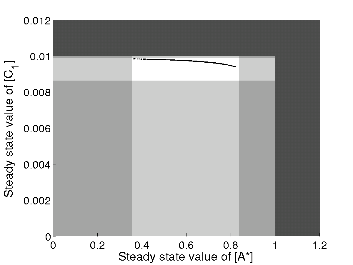
(a) Parameter uncertainty region $\mathcal{P}_{1}$ (2% variation)

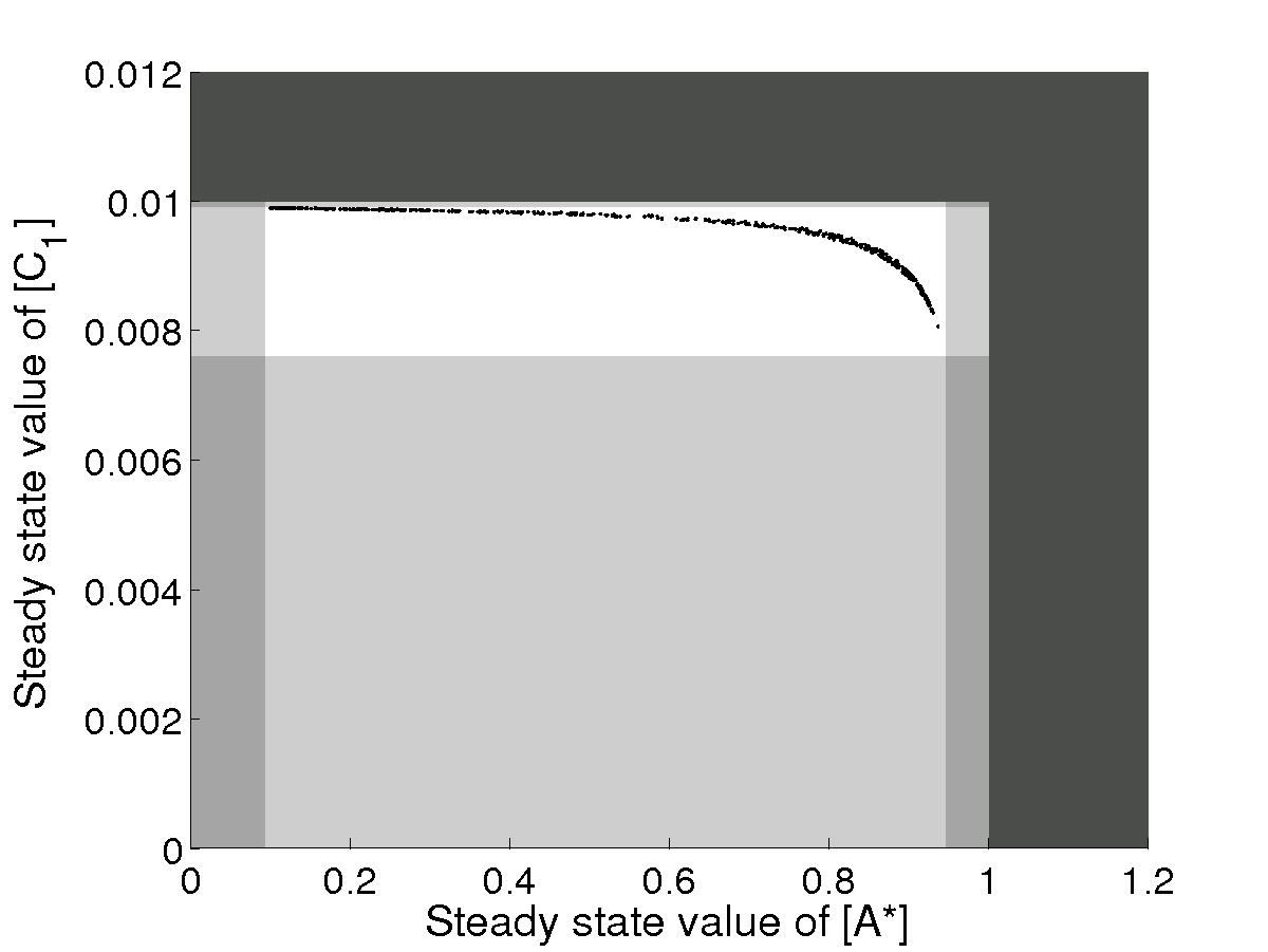
(b) Parameter uncertainty region $\mathcal{P}_{2}$ (10% variation)

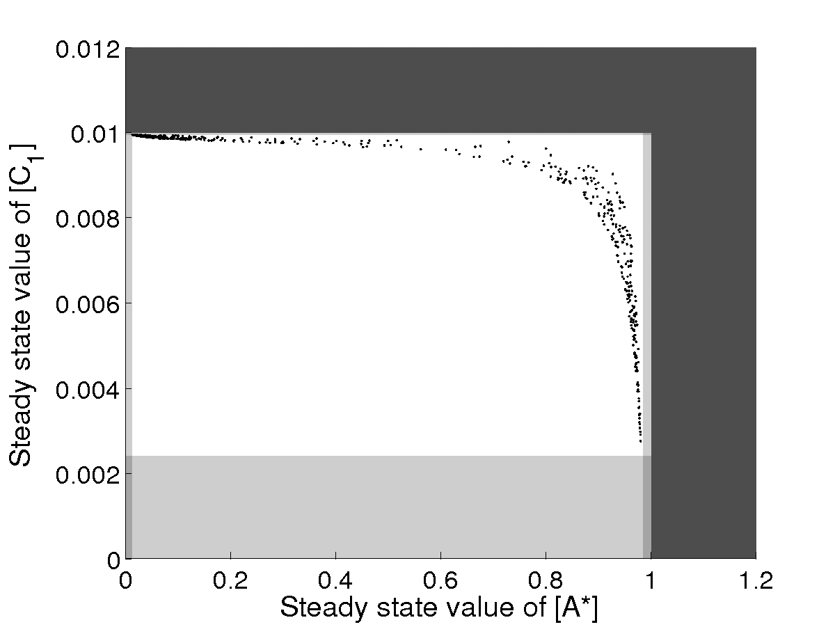
(c) Parameter uncertainty region $\mathcal{P}_{3}$ (2–fold variation)

Figure 1: Feasible steady states for the enzymatic cycle with three different parameter regions, comparison of reliable bounds obtained with Algorithm 1 and Monte–Carlo estimates. Light gray regions have been certified infeasible by Algorithm 1. Black dots are steady state values obtained from Monte-Carlo tests. Dark gray regions are known to be infeasible from conservation relations.

Our analysis also yields a biochemical interpretation, related to the property of ultrasensitivity. The concept of ultrasensitivity is quite important for biochemical reaction networks, in particular for those that constitute cellular signal transduction pathways [Levine et al., 2007]. Shortly, ultrasensitivity means that a small variation in a control variable has a relatively large effect on an output variable, whereas for increasing variations in the control variable, the range of the output variable will be considerably less increasing (see also Figure 2). Thus, ultrasensitivity is an inherently non-linear and non-local property. For the enzymatic cycle, a variation of only 2% in parameters already allows the steady state value of $[A^{\ast}]$ to vary over almost half of the interval given from the conservation relation, and with an allowable parameter variation of 10% the steady state value of $[A^{\ast}]$ can span nearly the whole interval. This is a clear indication of the ultrasensitivity which is typical for the enzymatic cycle [Goldbeter and Koshland, 1981].

Figure 2: Illustration of ultrasensitivity. Response of an output variable $x$ to a control variable $p$. The response is ultrasensitive, with high sensitivity around the nominal value $p_{0}$ and considerable less sensitivity for other values.

In addition, our results show that the steady state value of $[C_{1}]$, the concentration of the intermediate enzyme–substrate complex, is not ultrasensitive, because its value spans a large interval only for large parameter variations. Similar results hold for $[C_{2}]$.

6 Conclusions

We have studied the problem of computing the region of all steady states of biochemical reaction networks, provided that parameters are allowed to vary within a known region. This is an important problem in sensitivity analysis of reaction networks. Our approach is based on formulating a feasibility problem to check whether a candidate region in state space actually contains steady states. This feasibility problem is relaxed to a semidefinite program, and its Lagrangian dual provides certificates of infeasibility of a candidate region in state space. These certificates can be used to efficiently minimize the estimate of the known feasible region in state space by a bisection algorithm.

We have applied our sensitivity analysis to two simple example networks. For the first example, our algorithm is able to compute numerically exact bounds, which could be verified from the analytical solution. In the second example, we compared the bounds obtained from our algorithm to steady state values obtained through Monte–Carlo tests. In this example, our approach was more efficient computationally than Monte–Carlo tests. Also, it gives guaranteed bounds on the steady state values, which cannot be achieved by randomized methods such as Monte–Carlo tests. Based on the premise that we are working with hyperrectangles only, the obtained bounds are fairly tight. The second example also shows that our approach is able to confirm ultrasensitivity of the Goldbeter–Koshland switch.

In summary, our approach is a reliable and computationally efficient method to estimate the range of possible steady state variations due to multiple simultaneous parameter variations in biochemical reaction networks, and thus provides a valuable tool for global sensitivity analysis.

References

- Alves and Savageau [2000] R. Alves and M. A. Savageau. Systemic properties of ensembles of metabolic networks: application of graphical and statistical methods to simple unbranched pathways. Bioinformatics, 16(6):534–547, Jun 2000.
- Boyd and Vandenberghe [2004] S. Boyd and L. Vandenberghe. Convex optimization. Cambridge University Press, Cambridge, UK, 2004. URL http://www.stanford.edu/ boyd/cvxbook/.
- Feng et al. [2004] X.-J. Feng, S. Hooshangi, D. Chen, G. Li, R. Weiss, and H. Rabitz. Optimizing genetic circuits by global sensitivity analysis. Biophys. J., 87(4):2195–2202, Oct 2004. URL http://dx.doi.org/10.1529/biophysj.104.044131.
- Goldbeter and Koshland [1981] A. Goldbeter and D. E. Koshland. An amplified sensitivity arising from covalent modification in biological systems. Proc. Natl. Acad. Sci., 78(11):6840–44, Nov 1981.
- Kacser et al. [1995] H. Kacser, J. A. Burns, and D. A. Fell. The control of flux. Biochem. Soc. Trans., 23(2):341–366, 1995.
- Klipp et al. [2005] E. Klipp, R. Herwig, A. Kowald, Ch. Wierling, and H. Lehrach. Systems Biology in Practice. Concepts, Implementation and Application. Wiley-VCH Verlag, Weinheim, 2005. URL http://www3.interscience.wiley.com/cgi-bin/bookhome/110436350.
- Kuepfer et al. [2007] L. Kuepfer, U. Sauer, and P. Parrilo. Efficient classification of complete parameter regions based on semidefinite programming. BMC Bioinformatics, 8(1):12, Jan 2007. URL http://dx.doi.org/10.1186/1471-2105-8-12.
- Kuznetsov [1995] Y. A. Kuznetsov. Elements of Applied Bifurcation Theory. Springer-Verlag New York, 1995.
- Levine et al. [2007] J. Levine, H. Y. Kueh, and L. Mirny. Intrinsic fluctuations, robustness, and tunability in signaling cycles. Biophys. J., 92(12):4473–4481, Jun 2007. URL http://dx.doi.org/10.1529/biophysj.106.088856.
- Maranas and Floudas [1995] C. D. Maranas and C. A. Floudas. Finding all solutions of nonlinearly constrained systems of equations. J. Global Optim., 7(2):143–182, Sep 1995. URL http://dx.doi.org/10.1007/BF01097059.
- Neumaier [1990] A. Neumaier. Interval methods for systems of equations. Cambridge University Press, Cambridge, UK, 1990.
- Parrilo [2003] P. A. Parrilo. Semidefinite programming relaxations for semialgebraic problems. Mathematical Programming, 96(2):293–320, May 2003. URL http://dx.doi.org/10.1007/s10107-003-0387-5.
- Richter and DeCarlo [1983] S. L. Richter and R. A. DeCarlo. Continuation methods: theory and applications. IEEE Trans. Circ. Syst., 30(6):347–352, 1983.
- Robert and Casella [2004] C. P. Robert and G. Casella. Monte Carlo Statistical Methods. Springer-Verlag, 2004.
- Shacter et al. [1984] E. Shacter, P. B. Chock, and E. R. Stadtman. Regulation through phosphorylation/dephosphorylation cascade systems. J. Biol. Chem., 259(19):12252–59, Oct 1984.
- Streif et al. [2007] S. Streif, R. Findeisen, and E. Bullinger. Sensitivity analysis of biochemical reaction networks by bilinear approximation. In Proc. of the 2nd Foundations of Systems Biology in Engineering (FOSBE), pages 521–526, 2007.
- Vandenberghe and Boyd [1996] L. Vandenberghe and S. Boyd. Semidefinite programming. SIAM Review, 38(1):49–95, 1996. URL http://link.aip.org/link/?SIR/38/49/1.