Magnetism in tunable quantum rings

Abstract

We have studied the spin structure of circular four-electron quantum rings using tunable confinement potentials. The calculations were done using the exact diagonalization method. Our results indicate that ringlike systems can have oscillatory flips between ferromagnetic and antiferromagnetic behaviour as a function of the magnetic field. Furthermore, at constant external magnetic fields there were seen similar oscillatory changes between ferromagnetism and antiferromagnetism when the system parameters were changed. According to our results, the magnetism of quantum rings could be tuned by system parameters.

I Introduction

During the last two decades, there has been seen an increasing scientific and technological interest in spin related phenomena and in possible application of these in future data processing, communication and storage.Awschalom and Flatté (2007); Zutić et al. (2004) Quantum dots have been proposed as components in few-electron spintronics devices, such as spin filters or spin memories,Zutić et al. (2004); Recher et al. (2000) and in spin-based quantum computation devices.Loss and DiVincenzo (1998)

Existing fabrication techniques allow construction of semiconductor quantum rings of nanometer dimensions containing only a few electrons.Chakraborty (2003); Lorke et al. (2000); Hanson et al. (2007) Nanoscopic quantum rings are sufficiently small systems to show quantum effects, and large enough to be able to trap magnetic flux in their interior, when subjected to an experimentally reachable magnetic field. The trapping of magnetic flux quanta gives rise to interesting effects, such as persistent currents and other periodic properties related to the Aharonov–Bohm effect.Chakraborty (2003); Aharonov and Bohm (1959)

The main focus of this paper is on the magnetic properties of the quantum rings. The previous study by Koskinen et al.Koskinen et al. (2001) for one type of quantum rings has shown that a model of localized charges and antiferromagnetic coupling of the nearest-neighbor spins, corresponding to an antiferromagnetic Heisenberg model, captures the physics of systems they study. This means, for example, that when the angular momentum of the system is increased by making the magnetic field stronger, the change of the total spin of the system follows values found using the antiferromagnetic Heisenberg model. On the other hand, a study of a hard-wall quantum dotHancock et al. (2008) where strong electron-electron interaction forces the electron density to be ring-shaped, has found a ferromagnetic behavior of the system as a function of the magnetic field. Motivated by this discrepancy, we study tunable quantum rings and aim to identify the underlying physics that leads to different magnetic properties for the various quantum rings.

Our results show interestingly that the same quantum ring system can show oscillation between ferromagnetic and antiferromagnetic behavior as a function of the magnetic field. A similar control of the magnetism can be obtained by changing the width or the radius of the quantum ring.

II Model and computational Method

We use an effective-mass approximation and model the semiconductor quantum rings as two-dimensional systems with the Hamiltonian

$$H=\sum_{i=1}^{N}\bigg{(}\frac{(-i\hbar\nabla_{i}+e\mathbf{A}_{i})^{2}}{2m^{*}}+V(r_{i})\bigg{)}+\frac{e^{2}}{4\pi\epsilon}\sum_{i<j}^{N}\frac{C}{r_{ij}},$$ (1)

where $N$ is the number of electrons, $\mathbf{A}$ is the vector potential of the perpendicular magnetic field $\mathbf{B}=B\mathbf{u}_{z}$, $V$ is the external confinement potential, $m^{*}$ is the effective electron mass, $C$ is the Coulomb constant (normally 1), and $\epsilon$ is the dielectric constant. The electrons are restricted to the Cartesian $xy$ plane, and the magnetic field is normal to the plane. In our calculations, we use the effective parameter values of GaAs, namely, $m^{*}=$ 0.067$m_{e}$ and $\epsilon=$ 12.7. To enhance the spin effects, we have left out the Zeeman potential. This can be justified since experimentally the gyromagnetic factor, and thereby also the Zeeman term, can be made vanishingly small.Leadley et al. (1997)

To control the spin effects, we use confinement potentials of the form

$$V(r)=\frac{1}{2}m^{*}\omega_{0}^{2}r^{2}+V_{0}\exp(-r^{2}/\sigma^{2}),$$ (2)

where $\omega_{0}$ determines the confinement strength and $V_{0}$ determines the strength of the Gaussian perturbation. We set $\hbar\omega_{0}=$ 5 meV and $\sigma=$ 2 $a_{B}^{*}$, where $a_{B}^{*}\approx$ 10.03 nm is the effective Bohr radius of GaAs. By tuning the Gaussian perturbation stronger, we can make the system more and more ring-shaped. In addition, we have used a parabolic ring potential given by

$$V(r)=\frac{1}{2}m^{*}\omega_{0}^{2}(r-r_{0})^{2}$$ (3)

to model a narrow quantum ring.

In the exact diagonalization (ED) calculations, our single-particle states are the one-body eigenstates of the Hamiltonian $H$. In cases when the confinement potential $V$ is parabolic, the single-particle eigenstates are the Fock-Darwin states.Harju (2005) For systems with perturbed parabolic or parabolic ring potentials, we calculate the single-electron states as linear combinations of Fock-Darwin states, all with the same angular momentum, corresponding to the 15 lowest energy values. The ED calculations take into account Landau-level mixing, as the 25 lowest-lying eigenstates, irrespective of Landau level, are included in the computational procedure. The ground state eigenvalues of the Hamiltonian matrix of the ED method were obtained using the Lanczos diagonalization method, and the interaction matrix elements were calculated using numerical integration. The principles of the ED method are described in Ref. Gylfadottir et al., 2006.

When the electrons in a quantum ring become sufficiently localized, charge and spin excitations separate from each other.Koskinen et al. (2007) This phenomenon is a non-perturbative effect due to the strong correlations in quantum ring systems at high magnetic fields. The qualitative behavior of the many-particle spectrum of a quasi-one-dimensional system has been described by the lattice HamiltonianKoskinen et al. (2001); Viefers et al. (2004); Manninen and Reimann (2009)

$$H=J\sum_{i,j}\mathbf{S}_{i}\cdot\mathbf{S}_{j}+\frac{1}{2I}L^{2}+\sum_{\alpha}\hbar\omega_{\alpha}n_{\alpha},$$ (4)

where the first term is a Heisenberg Hamiltonian that models the spin degrees of freedom, the second term is a rigid rotation of the system, and the last term includes vibrational modes of the localized electrons. The parameters of the model are the nearest-neighbor coupling constant between the spins $J$, the total moment of inertia $I$, and the vibration frequency $\omega_{\alpha}$. The angular momentum of the ring is given by $L$ and $n_{\alpha}$ is the number of excitation quanta of the vibrational mode. In an antiferromagnetic system the coupling is such that $J>$ 0, and in a ferromagnetic system $J<$ 0.

The total angular momentum–spin pairs of the lowest eigenstates for the effective Hamiltonian (4) can be calculated using exact diagonalization, or using group-theoretical methods.Koskinen et al. (2001) In Table 1, we have given the angular momentum and spin states of the ferromagnetic and antiferromagnetic systems of four particles, as calculated by the exact diagonalization. The spin sequence is $N$-periodic as a function of the angular momentum, where $N$ is the number of electrons. One can see that for four particles, the antiferromagnetic behavior is manifested by the three consecutive ground states with spin equal to one, and one signature of the ferromagnetic model is the occurrence of ground state with spin equal to two. One should also note that there is one ground state with total spin equal to zero for both versions of the Heisenberg model.

Table 1: Total angular momenta $L$ and their corresponding spin values $S$ for the ferromagnetic and antiferromagnetic ground states of the Heisenberg model of a four-electron ring. Spin states corresponding to higher angular momenta are obtained by utilizing the periodicity of the spin sequence.

$L$		0	1	2	3
$S$	Ferromagnetic	0	1	2	1
$S$	Antiferromagnetic	1	1	0	1

III Results

III.1 Gaussian perturbation ring

We start with the results for the parabolic dot that has been perturbed with the Gaussian potential in the center to form a quantum ring.

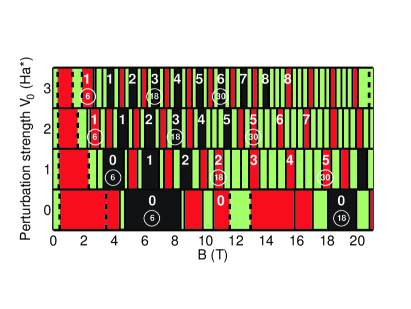
Figure 1: (Color online) Ground state spin polarization as a function of the magnetic field $B$ for a four-electron parabolic quantum dot with Gaussian perturbations of different strengths $V_{0}$. The spin states are 0 (red/middle grey), 1 (green/light grey), and 2 (dark grey). The upper integers denote the number of central vortices found in each of the different states, and the integers surrounded by a ring denote the corresponding angular momenta. All states at zero magnetic field have angular momentum 0. If two subsequent states are separated by a solid line, the angular momentum increases by one when moving to the state at right, and if they are separated by a dashed line, the angular momentum increases by two.

In Fig. 1, we have plotted spin ground states as a function of the magnetic field $B$ for four-electron perturbed parabolic dots with perturbation strengths $V_{0}=$ 0, 1, 2, and 3 Ha^∗ (1 Ha${}^{*}\approx$ 11.3036 meV). For all these perturbation strengths, the radius of the quantum ring is around 2 $a_{B}^{*}$. For $V_{0}=0$, corresponding to a pure parabolic quantum dot, the states with $L=6$ and 18 are the only fully spin-polarized states (dark gray regions in phase diagram), as also found in Ref. Koskinen et al., 2007 in the lowest Landau level approximation. The state with $L=6$ is called the maximum-density droplet (MDD),MacDonald et al. (1993) corresponding to the fractional quantum Hall states with filling fraction $\nu=1$, and the state with $L=18$ corresponds to $\nu=1/3$.Laughlin (1983) Between these two states the total spin has values of zero and one, but these do not follow the predictions from the antiferromagnetic Heisenberg model, most clearly seen from the fact that there are no regions with three consecutive ground states with spin equal to one. This is not surprising, as we expect the Heisenberg model to be relevant only in the limit where electrons are strongly in a ring-shaped confinement.

Next we turn on the Gaussian perturbation, and one can see that the spin-polarized state with $L=6$ at $V_{0}=0$ splits into several spin-polarized states with different angular momentum. In addition, between these $S=2$ states, the total spins follow the ferromagnetic Heisenberg spins given in Table 1. The only exception on this rule is found at $V_{0}=2$ around $B=11$ T, where $S=1$ is found instead 0.

Outside these ferromagnetic regions at stronger magnetic fields, one can see antiferromagnetic behavior. The antiferromagnetic phase can be identified by the three $S=1$ states in a row, separated by the $S=0$ state. In addition, antiferromagnetic behavior could develop at weak magnetic fields, as at $V_{0}=3$ there are already three consecutive states with $S=1$. As will be shown later in this paper, when the ring is sufficiently narrow there is indeed found an antiferromagnetic region at magnetic fields lower than the first ferromagnetic region.

In a previous studyHancock et al. (2008) of a hard-wall quantum dot with a radius $R=$ 5 $a_{B}^{*}$ and maximum of the electron density around 3 $a_{B}^{*}$, the spin structure was ferromagnetic for angular momenta $L$ between 6 and 18. Such a magnetic structure is almost the same as that found for the perturbed parabolic system with perturbations $V_{0}=$ 1 and 2. The magnetic structure of the wide quantum ring is thus for angular momenta 6 $\leq L\leq$ 18 similar to that of a hard-wall quantum dot.

III.2 Vortex structure

From the phase diagram shown in Fig. 1, one can also see that the state with angular momentum $L=6$ changes spin when the Gaussian impurity is made stronger. This change and many other details of the phase diagram can be understood by studying the vortex structure of the many-body wave function.

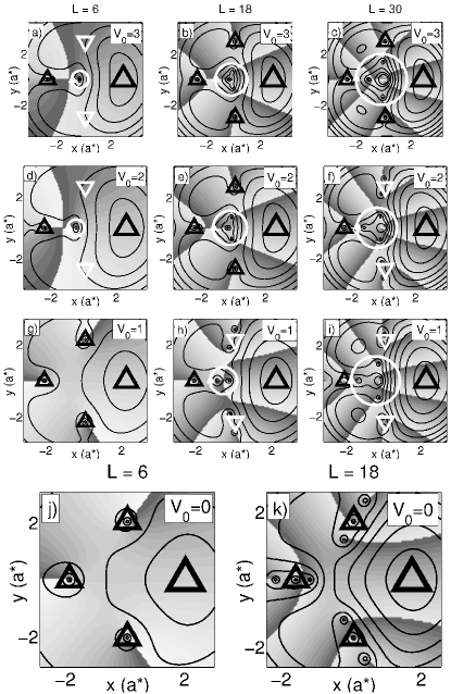
Figure 2: Conditional wave functions consisting of the charge density, plotted with contour lines (logarithmic scale), and the phase of the wave function, illustrated by the gray-scale shading. The fixed spin up electrons are marked with black triangles pointing up, and the spin down electrons with white triangles pointing down. The probe particle is marked with a larger triangle. The clusters consisting of central vortices (nodes), which can be considered as giant vortices, are denoted by circular arrows.

When subjected to an external magnetic field, the electrons in a quantum dot are forced to rotate. If the rotation is sufficiently strong, vortices are formed in the electron liquid.Saarikoski et al. (2004) One can consider the vortices as quasiparticles that are holes in the occupied Fermi sea.Manninen and Reimann (2009) The vortices are seen as zero points in the conditional electron density, where the phase of the wave function changes as a multiple of 2$\pi$ for a path enclosing the node. As shown in the fractional quantum Hall effect (FQHE) theory,Ezawa (2008) the formation of vortices is a result of quantization of the magnetic field, and each vortex is associated with an integer number of Dirac flux quanta.

To analyze the nodal structure of the perturbed quantum dot, we have calculated conditional wave functions,Saarikoski et al. (2004) defined for an $N$-particle system as

$$\psi_{c}(\mathbf{r})=\frac{\Psi(\mathbf{r},\mathbf{r}^{*}_{2},\dots,\mathbf{r}^{*}_{N})}{\Psi(\mathbf{r}^{*}_{1},\mathbf{r}^{*}_{2},\dots,\mathbf{r}^{*}_{N})},$$ (5)

where $\mathbf{r}$ is the position of the moved particle 1, and $\mathbf{r}_{i}^{*}$ is the most probable position of particle $i$ that are found by maximizing the total electron density $|\Psi|^{2}$. The phase $\theta$ is obtained from the relation $\psi_{c}(\mathbf{r})=|\psi_{c}(\mathbf{r})|\exp(i\theta(\mathbf{r}))$ and the conditional electron density is defined as $|\psi_{c}(\mathbf{r})|^{2}$.

Now returning to the question related to the spin of the $L=6$ state, a starting point for this analysis is the conditional wave function of the parabolic dot shown in Fig. 2(j). In this, one can see a Pauli vortex on top of each electron, except the probe particle on right. The vortices are shown by the discontinuous jumps in the gray-scale from white to black when the electrons are circulated in a clockwise fashion. The fact that the vortex number is the same as the electron number shows that the state is a finite-size example of a quantum Hall state with filling fraction $\nu=1$.

For $V_{0}=1$, shown in Fig. 2(g), the spin is still the same and the conditional wave function is nearly identical to the $V_{0}=0$ state. However, for $V_{0}=2$ the spin has changed from 2 to 0, and the conditional wave function in Fig. 2(d) looks completely different. There is still one Pauli vortex on top of the left-most electron, but the two other electrons have switched spins. In addition, there is now one vortex that is located at the center of the system. It turns out that one needs to combine two Pauli vortices in order to make one vortex at the center of the dot. From this data, one can understand the change in the total spin as follows: The system places the vortices so that it minimizes the total energy. Without the Gaussian impurity at the center of the dot, it is energetically favorable to place the vortices on top of the electrons to reduce the Coulomb repulsion. When the potential at the center of the dot is raised by the Gaussian impurity, at some strength it is more favorable to reduce the probability of the electrons to be at the center of the dot by placing a vortex there.

One can do a similar analysis for the $L=18$ state, which for $V_{0}=0$ corresponds to the $\nu=1/3$ state. The correspondence can be seen by the three vortices bound to each electron, as shown in Fig. 2(k). The reason for the small separation of the vortices is due to long-range nature of the interaction. For $V_{0}=1$ shown in Fig. 2(h), there are already two vortices at the center of the dot, and to create these, four Pauli vortices have vanished from the system. Due to this, the spin has again changed, and the opposite spins have only two vortices bound to them. As a general rule, opposite spin electrons can have even vortices bound to them, and the antisymmetry requirement of same spin electrons forces the vortex number to be odd. The vortex structure of the $S=0$ states is similar to that of a $\nu=2/3$ Halperin state,Chakraborty and Pietiläinen (1995); Girvin and MacDonald (1997); Halperin (1983) apart from the vortices at the center of the dot. Going to $V_{0}=2$ shown in Fig. 2(e), a third vortex has appeared at the center, and now again the total spin of the system has changed. Finally, at $V_{0}=3$ shown in Fig. 2(b) the conditional wave function is nearly identical to the $V_{0}=2$ case.

The same trend can be found at even larger values of the angular momentum, and as a final example, we show the data for the $L=30$ states in Figs. 2(c),(f), and (i). The main difference to the previous examples is that when the number of central vortices grows, also the area they occupy seems to be larger.

Analyzing the vortex structure of the other states in detail enables us to label the central vortex numbers of the ground states. These numbers are given in Fig. 1 for the most interesting states. One can see that in general, the number of central vortices grows as a function of the magnetic field. However, at each fixed Gaussian impurity strength, there is a point where it is energetically favorable to add Pauli vortices instead of the central vortices, and at this point the number of central vortices is constant although the angular momentum increases. At these points, the ferromagnetic behavior is changed to antiferromagnetic. Somewhat similar transitions are seen at the magnetic fields below the first ferromagnetic states.

It is also interesting to analyze the ground states at magnetic fields around 6–7 T. At $V_{0}=0$, the ground state is the $S=2$ state with $L=6$ corresponding to $\nu=1$. When the Gaussian impurity is made stronger, there are more and more vortices at the center of the system, and the angular momentum is increased. However, the spin of the ground state does not change. This shows that the $\nu=1$ state is in some sense stable even for this small particle number when one pierces it with three fluxes at the center. By this we mean that the vortex structure of the conditional wave function is the same apart from the central vortices, see Figs. 1(b) and (j).

III.3 Narrow quantum ring

Based on the analysis presented above, one would expect to find an antiferromagnetic region at low magnetic fields, if the ring is made sufficiently narrow (see the region with $B=$ 2–4 T and $V_{0}=$ 3 Ha^∗ of Fig. 1). To investigate this, we switch the confinement potential to

$$V(r)=\frac{1}{2}m^{*}\omega_{0}^{2}(r-r_{0})^{2},$$ (6)

where the confinement strength is taken to be 40 meV and the radius 8$a_{B}^{*}/\pi\approx 2.5a_{B}^{*}$. This system is a very narrow ring with approximately the same radius as the ring studied above.

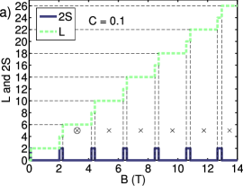
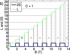
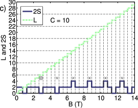
Figure 3: (Color online) Total angular momentum $L$ and spin $S$ of the ground states given as functions of the magnetic field $B$ for a four-electron parabolic ring with 40 meV confinement strength and radius 8$a_{B}^{*}$/$\pi$, where $a_{B}^{*}$ is the effective Bohr radius. The Coulomb constant is (a) $C=$ 0.1, (b) $C=$ 1, and (c) $C=$ 10. The crosses denote states with magic angular momenta $L_{k}=L_{\textrm{MDD}}+kN$, where $k\in\{0,1,2,\dots\}$, $L_{\textrm{MDD}}=(N-1)N/2$ is the angular momentum of the maximum-density droplet (MDD), and $N$ is the number of electrons. The state with angular momentum $L_{\textrm{MDD}}$ is marked with a cross surrounded by a circle.

In Fig. 3, the total angular momentum and spin of the ground state is plotted for the narrow ring. We have varied the Coulomb constant between the values $C=$ 0.1, 1, and 10. In reality, the interaction strength can be changed by changing the quantum ring radius.Gylfadottir et al. (2006) The case with $C=1$, shown in Fig. 3(b), corresponds to the natural interaction strength, and serves as basis for the comparison with the ring used above. For this case, the total spin has values zero and one, and above $B=4$ T there are three states with spin one between each ground state with spin equal to zero, in agreement with the antiferromagnetic Heisenberg model. Thus, as expected there is an antiferromagnetic region at low magnetic fields when the ring is sufficiently narrow.

When the Coulomb interaction is made weak by setting $C=0.1$, two of the three consecutive $S=1$ states are no longer ground states as shown in Fig. 3(a). Now, although the spin has values 0 and 1, the system does not behave as the antiferromagnetic model. This shows that the localization induced by the strong interaction is a necessity for antiferromagnetism.

On the other hand, when we make the interaction stronger by setting $C=10$, one can see that fully spin polarized ground states are found. In addition, the magnetic field range of each ground state is nearly the same. In the magnetic field region between 6 and 10 T, the ferromagnetism is not as pure as the antiferromagnetism for the $C=1$ case, as now the ground states with $S=0$ are missing. Also, the system is antiferromagnetic upto $B\approx 6$ T. We conclude that a transition between antiferromagnetic and ferromagnetic behaviour also can be controlled by the Coulomb interaction strength, or physically by tuning the radius of the quantum ring.

IV Conclusion

Our results indicate that both ferro- and antiferromagnetic phases are found for quantum rings in a strong magnetic field. In addition, the occurrence of the different magnetic phases are not trivial to predict, as the magnetic phase is determined by the magnetic field region, the ring width and the radius of the system. We found that the magnetic phase changes oscillatory as a function of the different system parameters. Knowledge of the nontrivial magnetic phase structure could be very fruitful for experiments, as the observed phenomena opens the possibility for tunability of the magnetism by changing system parameters. For example, in an experiment, a metallic electrode with adjustable voltage could be used to achieve the control we had in our calculations when using the Gaussian impurity.