The gauge theory of dislocations: a uniformly moving screw dislocation

Abstract

In this paper we present the equations of motion of a moving screw dislocation in the framework of the translation gauge theory of dislocations. In the gauge field theoretical formulation, a dislocation is a massive gauge field. We calculate the gauge field theoretical solutions of a uniformly moving screw dislocation. We give the subsonic and supersonic solutions. Thus, supersonic dislocations are not forbidden from the field theoretical point of view. We show that the elastic divergences at the dislocation core are removed. We also discuss the Mach cones produced by supersonic screw dislocations.

Keywords: dislocation dynamics; gauge theory of dislocations; supersonic motion.

1 Introduction

In the dynamics of dislocations it is usually assumed that the screw dislocation possesses a Lorentz symmetry (Frank, 1949; Hirth & Lothe, 1968; Günther, 1988) in contrast to the edge dislocation, which does not have a Lorentz-type symmetry because of two characteristic velocities, namely the velocities of transversal and longitudinal waves, entering the field equations. By means of such a Lorentz transformation, the screw dislocation can be transformed into a steady-state one like in Maxwell’s theory of electromagnetic fields. The question arises if the ‘classical’ dynamics of dislocations reproduces the correct behavior of dislocations. Usually, the conventional theories of dislocation dynamics have several drawbacks (e.g. inertial effects are missing, singularities). Unlike special relativity where the speed of light is an upper limit, in elastodynamics the speed of sound is not a limit velocity. Shock waves can move faster than the velocity of sound and form Mach cones. Similar predictions that dislocations can move faster than the speed of sound have been given in the literature based on the dynamics of dislocations (see, e.g., Eshelby (1956); Weertman (1967); Günther (1968, 1969); Weertman & Weertman (1980); Callias & Markenscoff (1980); Markenscoff & Huang (2008)) and computer simulations (Gumbsch & Gao, 1999; Koizumi et al., 2002; Li & Shi, 2002; Tsuzuki et al., 2008). Supersonic dislocations have been recently observed in plasma crystals (Nosenko et al., 2007).

Another question comes up whether dislocations cause symmetric or asymmetric force stresses. In classical dislocation theories the elastic distortion tensor is asymmetric and the force stress tensor is assumed to be symmetric. Due to this asymmetry between the distortion and the stress tensors, Kröner (1976) has introduced a modulus of rotation for the antisymmetric part of the force stress tensor. In addition, Hehl & Kröner (1965) and Kröner (1968) argued that dislocations produce moment stresses as response and antisymmetric force stresses. Pan & Chen (1994) calculated the antisymmetric stress corresponding to the body couple using nonlinear and linear continuum mechanics. Gao (1999) has developed an asymmetric theory of nonlocal elasticity based on an atomic lattice model and the three-dimensional quasicontinuum field theory. He pointed out that both strain and local rotation should be regarded as basic variables of geometric deformation and he has shown that the local rotation makes a very important contribution to the internal energy. For isotropic materials, the antisymmetric stress comes from the long range property of interaction of atoms in the metal materials and non-uniform distribution of atomic forces in the more microscopic structures (Gao, 1999).

A promising and straightforward candidate for an improved dynamical theory of dislocations is the so-called translational gauge theory of dislocations (Kadić & Edelen, 1983; Edelen & Lagoudas, 1988; Lazar & Anastassiadis, 2008, 2009). In the gauge theory of defects, dislocations arise naturally as a consequence of broken translational symmetry and their existence is not required to be postulated a priori. Moreover, such a theory uses the field theoretical framework which is well accepted in theoretical physics.

Recently, Sharma & Zhang (2006) have applied the gauge theory of dislocations to a uniformly moving screw dislocation. They derived a gauge field theoretical solution to the problem of a uniformly moving screw dislocation. However, we will show that their solution is not the correct one for a supersonic screw dislocation. First of all, they used the constitutive relations given by Kadić & Edelen (1983); Edelen & Lagoudas (1988), which are too simple. Even in Edelen’s version (Kadić & Edelen, 1983; Edelen & Lagoudas, 1988) of the gauge theory of dislocations there are at least three characteristic velocities. For the anti-plane strain problem of a screw dislocation Edelen’s theory possesses two characteristic velocities, namely the velocity of shear waves and a gauge theoretical characteristic velocity. This makes it impossible without further simplifications and arguments to use a Lorentz transformation or at least it is not possible to transform a moving screw dislocation into a steady-state dislocation. Nevertheless, Sharma & Zhang (2006) have constructed a solution of a screw dislocation using the Lorentz transformation with respect to a gauge theoretical characteristic velocity. In addition, they have considered the gauge theoretical characteristic velocity as an upper limit velocity. Finally, they solved the equations of motion of a screw dislocation in a steady state. The stress field of their solution does not possess the correct far field behavior because their solution is only given in terms of the characteristic gauge velocity and not in terms of the shear speed of sound. Neither no Mach cones appear in the supersonic regime. At best, the solution given by Sharma & Zhang (2006) is only valid in the subsonic regime if the characteristic gauge velocity is equal to the shear speed of sound.

In the meantime, Lazar & Anastassiadis (2008, 2009) have presented an improved translational gauge theoretical formulation of dislocations. They have used the correct isotropic constitutive relations in the gauge theory of dislocations which are incomplete and too simple in the books of Kadić & Edelen (1983) and Edelen & Lagoudas (1988). In the present paper we derive the equations of motion of a screw dislocation and we will solve them for a uniformly moving screw dislocation using the theory of Lazar & Anastassiadis (2008). We will show that a dislocation is a massive field in the gauge theoretical formulation. We will calculate subsonic and supersonic solutions of a uniformly moving screw dislocation.

2 Gauge theory of dislocations

In dislocation dynamics we have the following state quantities of dislocations (Kosevich, 1979; Landau & Lifschitz, 1989)

$$T_{ijk}=\beta_{ik,j}-\beta_{ij,k},\qquad I_{ij}=-v_{i,j}+{\dot{\beta}}_{ij}$$ (2.1)

called the dislocation density tensor and the dislocation current tensor, respectively. These are the kinematical quantities of dislocations and they are given in terms of the incompatible elastic distortion tensor $\beta_{ij}$ and incompatible physical velocity of the material continuum $v_{i}$. The dislocation density tensor describes the location and the shape of the dislocation core. The dislocation current tensor $I_{ij}$ describes the movement of the dislocation core and it contains rate terms ($v_{i,j}$ and $\dot{\beta}_{ij}$). The dislocation density and the dislocation current tensors have to satisfy the translational Bianchi identities (square brackets indicate skewsymmetrization)

$$\epsilon_{jkl}T_{ijk,l}=0,\qquad\dot{T}_{ijk}+2\,I_{i[j,k]}=0.$$ (2.2)

The first equation means that dislocations do not have sources and the second one represents that the circulation of the dislocation current is proportional to the time-derivative of the dislocation density. On the other hand, (2.2) are compatibility conditions ensuring that $T_{ijk}$ and $I_{ij}$ can be given in terms of $\beta_{ij}$ and $v_{i}$ according to (2.1).

In the dynamical translational gauge theory of dislocations the Lagrangian is of the bilinear form (linear theory)

$${\cal{L}}=T-W=\frac{1}{2}\,p_{i}v_{i}+\frac{1}{2}\,D_{ij}I_{ij}-\frac{1}{2}\,\sigma_{ij}\beta_{ij}-\frac{1}{4}\,H_{ijk}T_{ijk}.$$ (2.3)

Here, the canonical conjugate quantities (response quantities) are defined by

$$p_{i}:=\frac{\partial{\cal{L}}}{\partial v_{i}},\qquad\sigma_{ij}:=-\frac{\partial{\cal{L}}}{\partial\beta_{ij}},\qquad D_{ij}:=\frac{\partial{\cal{L}}}{\partial I_{ij}},\qquad H_{ijk}:=-2\frac{\partial{\cal{L}}}{\partial T_{ijk}},$$ (2.4)

where $p_{i}$, $\sigma_{ij}$, $I_{ij}$, and $H_{ijk}$ are the momentum vector, the force stress tensor, the dislocation momentum flux tensor, and the pseudomoment stress tensor, respectively.

The Euler-Lagrange equations derived from the total Lagrangian ${\cal{L}}={\cal{L}}(v_{i},\beta_{ij},I_{ij},T_{ijk})$ are given by

$$E^{\,{\boldsymbol{v}}}_{i}({\cal{L}})=\partial_{t}\frac{\partial{\cal{L}}}{\partial\dot{v}_{i}}+\partial_{j}\frac{\partial{\cal{L}}}{\partial v_{i,j}}-\frac{\partial{\cal{L}}}{\partial v_{i}}=0,$$ (2.5)

$$E^{\,\boldsymbol{\beta}}_{ij}({\cal{L}})=\partial_{t}\frac{\partial{\cal{L}}}{\partial\dot{\beta}_{ij}}+\partial_{k}\frac{\partial{\cal{L}}}{\partial\beta_{ij,k}}-\frac{\partial{\cal{L}}}{\partial\beta_{ij}}=0.$$ (2.6)

We add to ${\cal{L}}$ a so-called null Lagrangian, ${\cal{L}}_{N}=\sigma^{0}_{ij}\beta_{ij}-p^{0}_{i}v_{i}$, with the “background” stress $\sigma^{0}_{ij}$ and momentum $p^{0}_{i}$ as external source fields. Written in terms of the canonical conjugate quantities (2.4), Eqs. (2.5) and (2.6) take then the form

$$D_{ij,j}+p_{i} =p^{0}_{i},\qquad (\text{momentum balance of dislocations})$$ (2.7)

$$\dot{D}_{ij}+H_{ijk,k}+\sigma_{ij} =\sigma^{0}_{ij}\qquad (\text{stress balance of dislocations}).$$ (2.8)

Eqs. (2.7) and (2.8) represent the dynamical equations for the balance of dislocations. Eq. (2.7) is the momentum balance law of dislocations, where the physical momentum is the source of the dislocation momentum flux. Eq. (2.8) represents the stress balance of dislocations. Thus, the force stress and the time derivative of the dislocation momentum flux are the sources of the pseudomoment stress. The conservation of linear momentum appears as an integrability condition for the balance of dislocation equations. This can be seen by applying $\partial_{t}$ on (2.7) and $\partial_{j}$ on (2.8) and subtracting the last from the first one

$$\dot{p}_{i}-\sigma_{ij,j} =0,\qquad (\text{force balance of elasticity}),$$ (2.9)

where the time-derivative of the physical momentum is the source of the force stress.

The linear constitutive relations for the momentum, the asymmetric force stress, the dislocation momentum flux tensor and the pseudomoment stress of an isotropic and centrosymmetric medium are (Lazar & Anastassiadis, 2008)

$$p_{i} =\rho v_{i},$$ (2.10)

$$\sigma_{ij} =\lambda\delta_{ij}\beta_{kk}+\mu(\beta_{ij}+\beta_{ji})+\gamma(\beta_{ij}-\beta_{ji}),$$ (2.11)

$$D_{ij} =d_{1}\delta_{ij}I_{kk}+d_{2}(I_{ij}+I_{ji})+d_{3}(I_{ij}-I_{ji}),$$ (2.12)

$$H_{ijk} =c_{1}T_{ijk}+c_{2}(T_{jki}+T_{kij})+c_{3}(\delta_{ij}T_{llk}+\delta_{ik}T_{ljl}),$$ (2.13)

where $\rho$ is the mass density and with 9 material constants $\mu$, $\lambda$, $\gamma$, $c_{1},\dots,c_{3}$ and $d_{1},\dots,d_{3}$. Here $\mu$, $\lambda$ are the so-called Lamé coefficients, $\gamma$ denotes the modulus of rotation, $c_{1},\dots,c_{3}$ are higher-order stiffness parameters and $d_{1},\dots,d_{3}$ are related to higher-order inertia due to dislocations.

The requirement of non-negativity of the energy (material stability) $E=T+W\geq~{}0$ leads to the conditions of positive semi-definiteness of the material constants. Thus, the material parameters have to fulfill the following conditions (Lazar & Anastassiadis, 2008)

$$d_{2} \geq 0,\qquad d_{3} \geq 0,\qquad 3d_{1}+2d_{2} \geq 0,$$ (2.14)

$$\mu \geq 0,\qquad \gamma \geq 0,\qquad 3\lambda+2\mu \geq 0,$$ (2.15)

$$c_{1}-c_{2} \geq 0,\qquad c_{1}+2c_{2} \geq 0,\qquad c_{1}-c_{2}+2c_{3} \geq 0.$$ (2.16)

Substituting the constitutive equations in the above system (2.7) and (2.8), we obtain

$$d_{1}({\dot{\beta}}_{jj,i}-v_{j,ji})+(d_{2}+d_{3})({\dot{\beta}}_{ij,j}-v_{i,jj})+(d_{2}-d_{3})({\dot{\beta}}_{ji,j}-v_{j,ji})+p_{i}=p^{0}_{i},$$ (2.17)

$$d_{1}\delta_{ij}({\ddot{\beta}}_{kk}-{\dot{v}}_{k,k})+(d_{2}+d_{3})({\ddot{\beta}}_{ij}-{\dot{v}}_{i,j})+(d_{2}-d_{3})({\ddot{\beta}}_{ji}-{\dot{v}}_{j,i})$$

$$\quad+c_{1}(\beta_{ik,jk}-\beta_{ij,kk})+c_{2}(\beta_{ji,kk}-\beta_{jk,ik}+\beta_{kj,ik}-\beta_{ki,jk})+c_{3}\big{[}\delta_{ij}(\beta_{lk,lk}-\beta_{ll,kk})$$

$$\quad+(\beta_{kk,ji}-\beta_{kj,ki})\big{]}+\sigma_{ij}=\sigma^{0}_{ij},$$ (2.18)

which is a coupled system of partial differential equations for the field quantities ${\boldsymbol{v}}$ and $\boldsymbol{\beta}$.

3 Equations of motion of a screw dislocation

We now proceed to derive the equations of motion for a moving screw dislocation. The symmetry of a screw dislocation leaves only the following non-vanishing components of the physical velocity vector and elastic distortion tensor: $v_{z}$, $\beta_{zx}$, $\beta_{zy}$. The equations of motion of a moving screw dislocation read

$$(d_{2}+d_{3})(\dot{\beta}_{zx,x}+\dot{\beta}_{zy,y}-\Delta v_{z})+\rho v_{z} =\rho v^{0}_{z},$$ (3.1)

$$(d_{2}+d_{3})(\ddot{\beta}_{zx}-\dot{v}_{z,x})+c_{1}(\beta_{zy,xy}-\beta_{zx,yy})+(\mu+\gamma)\beta_{zx} =(\mu+\gamma)\beta^{0}_{zx},$$ (3.2)

$$(d_{2}-d_{3})(\ddot{\beta}_{zx}-\dot{v}_{z,x})+c_{2}(\beta_{zx,yy}-\beta_{zy,xy})+(\mu-\gamma)\beta_{zx} =(\mu-\gamma)\beta^{0}_{zx},$$ (3.3)

$$(d_{2}+d_{3})(\ddot{\beta}_{zy}-\dot{v}_{z,y})+c_{1}(\beta_{zx,xy}-\beta_{zy,xx})+(\mu+\gamma)\beta_{zy} =(\mu+\gamma)\beta^{0}_{zy},$$ (3.4)

$$(d_{2}-d_{3})(\ddot{\beta}_{zy}-\dot{v}_{z,y})+c_{2}(\beta_{zy,xx}-\beta_{zx,xy})+(\mu-\gamma)\beta_{zy} =(\mu-\gamma)\beta^{0}_{zy},$$ (3.5)

where $\Delta=\partial_{xx}+\partial_{yy}$. In addition, the equilibrium condition is given by

$$(\mu+\gamma)(\beta_{zx,x}+\beta_{zy,y})=\rho\dot{v}_{z}.$$ (3.6)

From the system of equations (3.2)–(3.5) we obtain the two relations

$$\frac{c_{1}}{\mu+\gamma} =-\frac{c_{2}}{\mu-\gamma},$$ (3.7)

$$\frac{d_{2}+d_{3}}{\mu+\gamma} =\frac{d_{2}-d_{3}}{\mu-\gamma}.$$ (3.8)

We may introduce the following quantities

$$\ell^{2}_{1} =\frac{c_{1}}{\mu+\gamma},$$ (3.9)

$$L^{2}_{1} =\frac{d_{2}+d_{3}}{\rho},$$ (3.10)

$$\tau^{2}_{1} =\frac{d_{2}+d_{3}}{\mu+\gamma}.$$ (3.11)

Here $\ell_{1}$ and $L_{1}$ are the ‘static’ and ‘dynamic’ characteristic length scales and $\tau_{1}$ is the characteristic time scale of the anti-plane strain problem. Moreover, $\ell_{1}$ is related to dislocation stiffness and $L_{1}$ is related to dislocation inertia. The velocity of elastic shear waves is defined in terms of the ‘dynamic’ length scale $L_{1}$ and the time scale $\tau_{1}$:

$$c^{2}_{T}=\frac{L_{1}^{2}}{\tau_{1}^{2}}=\frac{\mu+\gamma}{\rho}.$$ (3.12)

Due to the presence of $\gamma$ the velocity of elastic shear waves is greater than in a theory with symmetric force stresses. Moreover, the velocity of shear waves has a similar form in micropolar elasticity (see, e.g., Nowacki (1986)) where the force stress is also asymmetric. In a similar way, we may introduce the following transversal gauge-theoretical velocity defined in terms of $\ell_{1}$ and $\tau_{1}$:

$$a^{2}_{T}=\frac{\ell_{1}^{2}}{\tau_{1}^{2}}=\frac{c_{1}}{d_{2}+d_{3}},$$ (3.13)

and therefore

$$\frac{\ell_{1}^{2}}{L_{1}^{2}}=\frac{a_{T}^{2}}{c_{T}^{2}}.$$ (3.14)

In the case $\gamma=0$ we recover symmetric force stresses and from relations (3.7) and (3.8): $c_{1}=-c_{2}$ and $d_{3}=0$. It can be seen that $c_{1}=-c_{2}$ gives the inequalities (2.16) with $c_{1}\geq 0$ and $-c_{1}\geq 0$. Thus, for nonnegative $c_{1}$ and $c_{1}\neq 0$ we cannot fulfill (2.16). This is the price we have to pay for symmetric force stresses of a screw dislocation in the dislocation gauge theory.

Because we deal with the physical state quantities $({\boldsymbol{v}},\boldsymbol{\beta})$, no pseudo-Lorentz gauge (Kadić & Edelen, 1983; Edelen & Lagoudas, 1988) is used and allowed during the simplification of the equations of motion. Gauge conditions are only allowed for gauge potentials and not for physical state quantities. Of course, for anti-plane strain the equilibrium condition (3.6) together with (3.12) looks like a ‘gauge’ condition but it is not a gauge condition from the physical interpretation.

Applying the equilibrium condition (3.6), the equations of motion (3.1)–(3.5) can be written in the form

$$\tau_{1}^{2}\ddot{v}_{z}-L_{1}^{2}\Delta v_{z}+v_{z} =v^{0}_{z},$$ (3.15)

$$\tau_{1}^{2}\ddot{\beta}_{zx}-\ell_{1}^{2}\Delta\beta_{zx}-\tau_{1}^{2}\Big{(}1-\frac{\ell_{1}^{2}}{L_{1}^{2}}\Big{)}\dot{v}_{z,x}+\beta_{zx} =\beta^{0}_{zx},$$ (3.16)

$$\tau_{1}^{2}\ddot{\beta}_{zy}-\ell_{1}^{2}\Delta\beta_{zy}-\tau_{1}^{2}\Big{(}1-\frac{\ell_{1}^{2}}{L_{1}^{2}}\Big{)}\dot{v}_{z,y}+\beta_{zy} =\beta^{0}_{zy}.$$ (3.17)

These are the equations of motion of an arbitrary moving screw dislocation in the framework of dislocation gauge theory. Some important questions arise if the lengths $\ell_{1}$ and $L_{1}$ are independent or not and is there a physical reason to decouple the field equations (3.15)–(3.17).

Consider a screw dislocation moving in the $x$-direction. If we want to construct a solution which is consistent with the classical solution, we have to fulfill the condition: $I_{zx}^{0}=-v^{0}_{z,x}+\dot{\beta}^{0}_{zx}=0$, because only the classical dislocation density $T^{0}_{zxy}$ and dislocation current $I^{0}_{zy}$ are non-zero. If we use the field equations (3.15) and (3.16), we obtain:

$$-\Big{[}\frac{\ell_{1}^{2}}{c_{T}^{2}}\,\partial_{tt}-L_{1}^{2}\Delta+1\Big{]}v_{z,x}+\Big{[}\frac{L_{1}^{2}}{c_{T}^{2}}\,\partial_{tt}-\ell_{1}^{2}\Delta+1\Big{]}\dot{\beta}_{zx}=0.$$ (3.18)

To guarantee that (3.18) is fulfilled, we choose

$$v_{z,x}=\dot{\beta}_{zx},\qquad{\text{and}}\qquad L_{1}=\ell_{1}.$$ (3.19)

Equation (3.19a) ensures that $I_{zx}=0$ and (3.19b) with (3.14) gives the relation $a_{T}=c_{T}$, which means that only one characteristic velocity $c_{T}$ survives for a screw dislocation in the gauge theory of dislocations. Thus, for a physically consistent solution we obtain the uncoupled Klein-Gordon equations

$$\big{[}1+\ell_{1}^{2}\square_{T}\big{]}v_{z}=v^{0}_{z},$$ (3.20)

$$\big{[}1+\ell_{1}^{2}\square_{T}\big{]}\beta_{zx}=\beta^{0}_{zx},$$ (3.21)

$$\big{[}1+\ell_{1}^{2}\square_{T}\big{]}\beta_{zy}=\beta^{0}_{zy},$$ (3.22)

with the following $(1+2)$-dimensional d’Alembert operator (wave operator)

$$\square_{T} =\frac{1}{c^{2}_{T}}\,\partial_{tt}-\Delta.$$ (3.23)

Moreover, the uncoupled system  (3.20)–(3.22) with only one characteristic velocity possesses a Lorentz symmetry. However, $c_{T}$ is not a limit velocity unlike the speed of light in special relativity. In field theories, Klein-Gordon equations describe massive fields (see, e.g., Rubakov (2002)). Thus, a dislocation is a massive gauge field. From the condition $L_{1}=\ell_{1}$, we find for the inertia term of a screw dislocation

$$d_{2}+d_{3}=\frac{c_{1}}{c^{2}_{T}}=\rho\,\ell^{2}_{1},$$ (3.24)

that it is given in terms of the characteristic length scale $\ell_{1}$. Under these assumptions, the dynamical dislocation gauge theory of a screw dislocation possesses only one internal length scale $\ell_{1}$.

If we multiply Eqs. (3.20)–(3.22) with $\square_{T}$ and using the ‘classical’ result (Günther, 1968, 1969), we obtain

$$\big{[}1+\ell_{1}^{2}\square_{T}\big{]}\square_{T}v_{z}=I^{0}_{zy,y},$$ (3.25)

$$\big{[}1+\ell_{1}^{2}\square_{T}\big{]}\square_{T}\beta_{zx}=T^{0}_{zxy,y},$$ (3.26)

$$\big{[}1+\ell_{1}^{2}\square_{T}\big{]}\square_{T}\beta_{zy}=-T^{0}_{zxy,x}+\frac{1}{c_{T}^{2}}\dot{I}^{0}_{zy},$$ (3.27)

as a set of fourth-order partial differential equations. As source terms only the classical dislocation density $T^{0}_{zxy}$ and dislocation current $I^{0}_{zy}$ are acting. Eqs. (3.25)–(3.27) have the two-dimensional form of Bopp-Podolsky equations (Bopp, 1940; Podolsky, 1942) (see also Iwanenko & Sokolow (1953)) in generalized electrodynamics, introduced by Bopp and Podolsky in order to avoid singularities in electrodynamics.

In general, the velocity $V$ of a screw dislocation might be subsonic or supersonic relative to the material space. A subsonic velocity lies in the range: $0<V<c_{T}$ and for supersonic screw dislocations the velocity reads: $c_{T}<V$.

4 Uniformly moving screw dislocation

We now study a screw dislocation moving with a uniform velocity $V$ in the $x$-direction. Here $V$ denotes the dislocation velocity in the material space. The dislocation moves relative to the material space, which plays the role of an ‘aether’. If a screw dislocation is moving with the velocity $V$, then $v_{z}$ is the physical velocity of the material space, where the dislocation lives in, in order to transport the dislocation core to another position in the material space. Let $x^{\prime}$ be the coordinate in the direction of motion in the moving coordinate system. For the uniformly moving screw dislocation, then we use the transform

$$x^{\prime}=x-Vt$$ (4.1)

with

$$\partial_{t}=-V\partial_{x^{\prime}}$$ (4.2)

and we obtain the equations

$$\big{[}1-\ell_{1}^{2}\big{(}(1-M^{2}_{T})\partial_{x^{\prime}x^{\prime}}+\partial_{yy}\big{)}\big{]}v_{z}=v^{0}_{z},$$ (4.3)

$$\big{[}1-\ell_{1}^{2}\big{(}(1-M^{2}_{T})\partial_{x^{\prime}x^{\prime}}+\partial_{yy})\big{]}\beta_{zx}=\beta^{0}_{zx},$$ (4.4)

$$\big{[}1-\ell_{1}^{2}\big{(}(1-M^{2}_{T})\partial_{x^{\prime}x^{\prime}}+\partial_{yy}\big{)}\big{]}\beta_{zy}=\beta^{0}_{zy},$$ (4.5)

and

$$\big{[}1-\ell_{1}^{2}\big{(}(1-M^{2}_{T})\partial_{x^{\prime}x^{\prime}}+\partial_{yy}\big{)}\big{]}T_{zxy}=T^{0}_{zxy},$$ (4.6)

$$\big{[}1-\ell_{1}^{2}\big{(}(1-M^{2}_{T})\partial_{x^{\prime}x^{\prime}}+\partial_{yy}\big{)}\big{]}I_{zy}=I^{0}_{zy},$$ (4.7)

with the Mach number of a moving screw dislocation relative to $c_{T}$:

$$M_{T}=\frac{V}{c_{T}}.$$ (4.8)

Eqs. (4.3)–(4.7) are two-dimensional modified inhomogeneous Helmholtz equations (subsonic case). In the supersonic case they change to one-dimensional inhomogeneous Klein-Gordon equations (see below).

4.1 Subsonic case

We now study a screw dislocation moving with a uniform velocity $V<c_{T}$ in the $x$-direction ($M_{T}<1$). The ‘background’ solution reads (see, e.g., Günther (1968))

$$v^{0}_{z}=V\partial_{y}F^{0},\qquad\beta^{0}_{zx}=-\partial_{y}F^{0},\qquad\beta^{0}_{zy}=\beta_{T}^{2}\partial_{x}F^{0},$$

$$T^{0}_{zxy}=b\delta(x-Vt)\delta(y),\qquad I^{0}_{zy}=-bV\delta(x-Vt)\delta(y),$$ (4.9)

with

$$F^{0}=\frac{b}{2\pi}\frac{1}{\beta_{T}}\,\ln r_{T}$$ (4.10)

and

$$r_{T} =\sqrt{(x-Vt)^{2}+\beta_{T}^{2}y^{2}},\qquad\beta_{T}=\sqrt{1-M^{2}_{T}}.$$ (4.11)

In the subsonic region, the field equations (4.3)–(4.7) are:

$$\big{[}1-\ell_{1}^{2}(\beta_{T}^{2}\partial_{x^{\prime}x^{\prime}}+\partial_{yy})\big{]}v_{z}=v^{0}_{z},$$ (4.12)

$$\big{[}1-\ell_{1}^{2}(\beta_{T}^{2}\partial_{x^{\prime}x^{\prime}}+\partial_{yy})\big{]}\beta_{zx}=\beta^{0}_{zx},$$ (4.13)

$$\big{[}1-\ell_{1}^{2}(\beta_{T}^{2}\partial_{x^{\prime}x^{\prime}}+\partial_{yy})\big{]}\beta_{zy}=\beta^{0}_{zy},$$ (4.14)

and

$$\big{[}1-\ell_{1}^{2}\big{(}\beta^{2}_{T}\partial_{x^{\prime}x^{\prime}}+\partial_{yy}\big{)}\big{]}T_{zxy}=T^{0}_{zxy},$$ (4.15)

$$\big{[}1-\ell_{1}^{2}\big{(}\beta^{2}_{T}\partial_{x^{\prime}x^{\prime}}+\partial_{yy}\big{)}\big{]}I_{zy}=I^{0}_{zy}.$$ (4.16)

Eqs. (4.12)–(4.16) can be easily solved with the inhomogeneous parts (4.1) using Fourier transform or other techniques. The solutions for the dislocation density and the dislocation flux of a screw dislocation are given by

$$T_{zxy} =\frac{b}{2\pi}\frac{1}{\ell^{2}_{1}\beta_{T}}\,K_{0}\Big{(}\frac{r_{T}}{\ell_{1}\beta_{T}}\Big{)},$$ (4.17)

$$I_{zy} =-\frac{b}{2\pi}\frac{V}{\ell^{2}_{1}\beta_{T}}\,K_{0}\Big{(}\frac{r_{T}}{\ell_{1}\beta_{T}}\Big{)}.$$ (4.18)

(a) (b)

Figure 1: Contourplot of the dislocation density $T_{zxy}$ of a screw dislocation moving with subsonic speed: (a) $V=0.1c_{T}$, (b) $V=0.9c_{T}$.

Here, the symbol $K_{n}$ stands for the modified Bessel function of second kind (McDonald function) and of order $n$. In Fig. 1 the dislocation density is plotted for different speeds subsonic with respect to $c_{T}$. The field of the dislocation density suffers a contraction when the value of its velocity approaches the velocity $c_{T}$. The curve of $T_{zxy}$ is a circle at $V=0$ and is a generalized ellipse at any other velocity $V<c_{T}$. The field is dilated in the directions orthogonal to the direction of motion and contracted along the line of motion. The solution for the elastic velocity is given by

$$v_{z} =\frac{b}{2\pi}\frac{\beta_{T}Vy}{r_{T}^{2}}\Big{[}1-\frac{r_{T}}{\ell_{1}\beta_{T}}\,K_{1}\Big{(}\frac{r_{T}}{\ell_{1}\beta_{T}}\Big{)}\Big{]}.$$ (4.19)

In Figs. 2 and 3 the physical velocity of a screw dislocations is plotted for subsonic velocities. It shows again a Fitzgerald contraction. It does not have a singularity. The physical velocity possesses extremum values depending on the dislocation velocity near the dislocation line.

(a) (b)

Figure 2: Contourplot of the elastic velocity $v_{z}$ of a screw dislocation moving with subsonic speed: (a) $V=0.1c_{T}$, (b) $V=0.9c_{T}$.

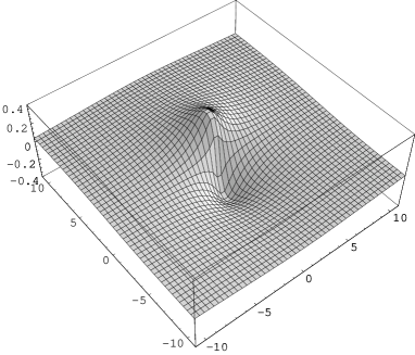
Figure 3: Three-dimensional plots of the physical velocity $v_{z}$ in units of $bV/2\pi\ell_{1}^{2}\beta_{T}$: (a) $V=0.1c_{T}$, (b) $V=0.9c_{T}$.

The solution of the elastic distortion reads

$$\beta_{zx} =-\frac{b}{2\pi}\frac{\beta_{T}y}{r_{T}^{2}}\Big{[}1-\frac{r_{T}}{\ell_{1}\beta_{T}}\,K_{1}\Big{(}\frac{r_{T}}{\ell_{1}\beta_{T}}\Big{)}\Big{]},$$ (4.20)

$$\beta_{zy} =\frac{b}{2\pi}\frac{\beta_{T}(x-Vt)}{r_{T}^{2}}\Big{[}1-\frac{r_{T}}{\ell_{1}\beta_{T}}\,K_{1}\Big{(}\frac{r_{T}}{\ell_{1}\beta_{T}}\Big{)}\Big{]}.$$ (4.21)

All the elastic fields are nonsingular in the gauge theoretical framework.

On the other hand, the solution (4.20) and (4.21) has the same form as the expression given by Sharma & Zhang (2006) if $c_{T}=a_{T}$ and $\gamma=0$.

4.2 Supersonic case

We now consider the supersonic case: $V>c_{T}$, (the supersonic case: $M_{T}>1$). Therefore, the term $\beta^{2}_{T}=-\gamma^{2}_{T}$ alters where

$$\gamma_{T}=\sqrt{M^{2}_{T}-1}.$$ (4.22)

Then the field equation for the dislocation density changes to

$$\big{[}1+\ell_{1}^{2}(\gamma_{T}^{2}\partial_{x^{\prime}x^{\prime}}-\partial_{yy})\big{]}T_{zxy}=T^{0}_{zxy}.$$ (4.23)

It is an inhomogeneous one-dimensional Klein-Gordon equation. The dislocation density of a supersonic screw dislocation has the form of the corresponding Green function. Therefore, it is given by (see, e.g., Iwanenko & Sokolow (1953))

$$T_{zxy}=\frac{b}{2\ell_{1}^{2}\gamma_{T}}\,J_{0}\bigg{(}\frac{\sqrt{(Vt-x)^{2}-\gamma_{T}^{2}y^{2}}}{\ell_{1}\gamma_{T}}\bigg{)}\,H((Vt-x)-\gamma_{T}|y|).$$ (4.24)

Here, the symbol $J_{n}$ denotes the Bessel function of first kind and of order $n$ and $H$ is the Heaviside step function. It is non-zero just for $Vt-x>\gamma_{T}|y|$. It builds a shear-wave Mach cone with the angle $\sin\theta_{T}=\frac{c_{T}}{V}$. The dislocation density has a maximum of $T_{zxy}=b/[2\gamma_{T}\ell_{1}^{2}]$ on the Mach cone. Inside the Mach cone it oscillates with decreasing amplitude. For the dislocation current density we obtain $I_{zy}=-V\,T_{zxy}$ with (4.24). The visualization of the Mach cone of the dislocation density $T_{zxy}$ produced by the screw dislocation in the supersonic regime is plotted in Fig. 4.

Figure 4: Contourplot of the dislocation density $T_{zxy}$ of a screw dislocation moving with supersonic speed $V=\sqrt{2}c_{T}$.

The equations of the elastic fields, altering their character from elliptic to hyperbolic, are

$$\big{[}1+\ell_{1}^{2}(\gamma_{T}^{2}\partial_{x^{\prime}x^{\prime}}-\partial_{yy})\big{]}v_{z}=v_{z}^{0},$$ (4.25)

$$\big{[}1+\ell_{1}^{2}(\gamma_{T}^{2}\partial_{x^{\prime}x^{\prime}}-\partial_{yy})\big{]}\beta_{zx}=\beta_{zx}^{0},$$ (4.26)

$$\big{[}1+\ell_{1}^{2}(\gamma_{T}^{2}\partial_{x^{\prime}x^{\prime}}-\partial_{yy})\big{]}\beta_{zy}=\beta^{0}_{zy},$$ (4.27)

with the inhomogeneous parts (A.4)–(A.6). The corresponding solutions read

$$v_{z} =\frac{bV}{2\ell_{1}}\,\frac{y}{\sqrt{(Vt-x)^{2}-\gamma_{T}^{2}y^{2}}}\,J_{1}\bigg{(}\frac{\sqrt{(Vt-x)^{2}-\gamma_{T}^{2}y^{2}}}{\ell_{1}\gamma_{T}}\bigg{)}\,H((Vt-x)-\gamma_{T}|y|),$$ (4.28)

$$\beta_{zx} =-\frac{b}{2\ell_{1}}\,\frac{y}{\sqrt{(Vt-x)^{2}-\gamma_{T}^{2}y^{2}}}\,J_{1}\bigg{(}\frac{\sqrt{(Vt-x)^{2}-\gamma_{T}^{2}y^{2}}}{\ell_{1}\gamma_{T}}\bigg{)}\,H((Vt-x)-\gamma_{T}|y|),$$ (4.29)

$$\beta_{zy} =-\frac{b}{2\ell_{1}}\,\frac{(Vt-x)}{\sqrt{(Vt-x)^{2}-\gamma_{T}^{2}y^{2}}}\,J_{1}\bigg{(}\frac{\sqrt{(Vt-x)^{2}-\gamma_{T}^{2}y^{2}}}{\ell_{1}\gamma_{T}}\bigg{)}\,H((Vt-x)-\gamma_{T}|y|).$$ (4.30)

It can be seen that (4.28) is non-zero just for $Vt-x>\gamma_{T}|y|$. Also it builds a shear-wave Mach cone with the angle $\sin\theta_{T}=\frac{c_{T}}{V}$. It is important to note that the classical singularity as Dirac delta function of supersonic dislocations on the Mach cone does not appear in our gauge theoretical result. The elastic distortions and the velocity have a maximum value on the Mach cone: $v_{z}=bVy/[4L_{1}^{2}\gamma_{T}]$, $\beta_{zx}=-by/[4\ell_{1}^{2}\gamma_{T}]$, $v_{z}$ and $\beta_{zx}$ are also zero at $y=0$. Inside the Mach cone they oscillate with decreasing amplitude. The visualization of the Mach cone of the physical velocity $v_{z}$ produced by the screw dislocation in the supersonic regime is plotted in Fig. 5.

Figure 5: Contourplot of the physical velocity $v_{z}$ of a screw dislocation moving with supersonic speed $V=\sqrt{2}c_{T}$.

Let us mention that the solution of Sharma & Zhang (2006) does not possess the correct behavior in the supersonic region. The solution given by Sharma & Zhang (2006) does not show Mach cones, which are predicted in computer simulations (Gumbsch & Gao, 1999; Koizumi et al., 2002; Li & Shi, 2002; Tsuzuki et al., 2008) and found experimentally (Nosenko et al., 2007).

5 Conclusion

In this paper, we have investigated a moving screw dislocation in the gauge field theory of dislocations. We derived the equations of motion of an arbitrary moving screw dislocation in this field-theoretical framework. First, a coupled system of inhomogeneous Klein-Gordon equations is obtained in the dynamical case with two characteristic velocities. We have found one dynamical characteristic length scale $L_{1}$, one static characteristic length scale $\ell_{1}$ and one characteristic time scale $\tau_{1}$. Later we have decoupled the field equations, following physical arguments, to construct a consistent solution. Due to these arguments we found $L_{1}=\ell_{1}$ and $a_{T}=c_{T}$. The elastic fields $v_{z}$, $\beta_{zx}$ and $\beta_{zy}$ and the fields of the dislocation core $T_{zxy}$ and $I_{zy}$ have the characteristic speed $c_{T}$. For a uniformly moving screw dislocation we have given analytical solutions for the subsonic and supersonic cases. For the supersonic case we found one Mach cone for the velocities $c_{T}$.

Appendix A Supersonic screw dislocation in elasticity

In the elasticity, a supersonic screw dislocation moves with the velocity: $V>c_{T}$. In symmetric elasticity the speed of shear waves reads: $c^{2}_{T}=\mu/\rho$ and in asymmetric elasticity it is given by $c^{2}_{T}=(\mu+\gamma)/\rho$. In asymmetric elasticity the antisymmetric part of the stress tensor produces body couples. The field equations for the elastic velocity and the elastic distortions read (Günther, 1968)

$$\square_{T}v_{z}^{0}=-bV\,\partial_{y}\delta(x-Vt)\delta(y),$$ (A.1)

$$\square_{T}\beta_{zx}^{0}=b\,\partial_{y}\delta(x-Vt)\delta(y),$$ (A.2)

$$\square_{T}\beta_{zy}^{0}=b\,\gamma^{2}_{T}\partial_{x}\delta(x-Vt)\delta(y).$$ (A.3)

These are inhomogeneous wave equations describing massless fields. The supersonic solutions are

$$v_{z}^{0} =\frac{bV}{2}\frac{y}{|y|}\,\delta(Vt-x-\gamma_{T}|y|),$$ (A.4)

$$\beta_{zx}^{0} =-\frac{b}{2}\frac{y}{|y|}\,\delta(Vt-x-\gamma_{T}|y|),$$ (A.5)

$$\beta_{zy}^{0} =-\frac{b\,\gamma_{T}}{2}\,\delta(Vt-x-\gamma_{T}|y|),$$ (A.6)

where $\delta$ denotes the Dirac delta function. Thus, the classical solutions are shock waves produced by a supersonic screw dislocation. Both in front of and behind the shock front the material is undeformed and at rest.

References

- Askes & Aifantis (2006) Askes, H. & Aifantis, E.C. 2006 Gradient elasticity theories in statics and dynamics – a unification of approaches. Int. J. Fract. 139, 297–304.
- Askes et al. (2007) Askes, H., Bennett, T. & Aifantis, E.C. 2007 A new formulation and -implementation of dynamically consistent gradient elasticity. Int. J. Meth. Engng. 72, 111–126.
- Bopp (1940) Bopp, F. 1940 Die lineare Theorie des Elektrons. Ann. Phys. (Leipzig) 38, 345–384.
- Callias & Markenscoff (1980) Callias, C. & Markenscoff, X. 1980 The nonuniform motion of a supersonic dislocation. Q. Appl. Math. 38, 323–330.
- Edelen & Lagoudas (1988) Edelen, D.G.B. & Lagoudas, D.C. 1988 Gauge theory and defects in solids. in: Mechanics and Physics of Discrete System. Vol. 1. North-Holland, Amsterdam.
- Edelen (1996) Edelen, D.G.B. 1996 A correct, globally defined solution of the screw dislocation problem in the gauge theory of defects. Int. J. Engng. Sci. 34, 81–86.
- Eshelby (1956) Eshelby, J.D. 1956 Supersonic dislocations and dislocations in dispersive media. Proc. Phys. Soc. B 69, 1013–1019.
- Frank (1949) Frank, F.C. 1949 On the equations of motion of crystal dislocations. Proc. Phys. Soc. (London) A 62, 131–134.
- Gao (1999) Gao, J. 1999 An asymmetric theory of nonlocal elasticity – Part 1. Quasicontinuum theory. Int. J. Solids Struct. 36, 2947–2958.
- Gitman et al. (2005) Gitman, I.M., Askes, H. & Aifantis, E.C. 2005 The representation volume size in static and dynamic micro-macro transitions. Int. J. Fract. 135, L3–L9.
- Gumbsch & Gao (1999) Gumbsch, R. & Gao, H. 1999 Dislocations faster than the speed of sound. Science 283, 965–968.
- Günther (1968) Günther, H. 1968 Überschallbewegung von Eigenspannungsquellen in der Kontinuumstheorie. Ann. Phys. (Leipzig) 21, 93–105.
- Günther (1969) Günther, H. 1969 Zur Theorie der Überschall-Eigenspannungsquellen. Ann. Phys. (Leipzig) 24, 82–93.
- Günther (1988) Günther, H. 1988 On Lorentz symmetries in solids. Phys. stat. sol. (b) 149, 101–109.
- Hehl & Kröner (1965) Hehl, F.W. & Kröner, E. 1965 Zum Materialgesetz eines elastische Mediums mit Momentenspannungen. Z. Naturforschg. 20a, 336-350.
- Hirth & Lothe (1968) Hirth, J.P. & Lothe, J. 1968 Theory of Dislocations. McGraw-Hill, New York.
- Iwanenko & Sokolow (1953) Iwanenko, D. & Sokolow, A. 1953 Klassische Feldtheorie. Akademie-Verlag: Berlin.
- Kadić & Edelen (1983) Kadić, A. & Edelen, D.G.B. 1983 A Gauge Theory of Dislocations and Disclinations. in: Lecture Notes in Physics. Vol. 174, Springer, Berlin.
- Koizumi et al. (2002) Koizumi, H., Kirchner, H.O.K. & Suzuki, T. 2002 Lattice wave emissions from a moving dislocation. Phys. Rev. B 65, 214104-1–9.
- Kosevich (1979) Kosevich, A.N. 1979 Crystal Dislocations and the Theory of Elasticity. in: Dislocations in Solids Vol. 1. F.R.N. Nabarro, ed., North-Holland, pp. 33-165.
- Kröner (1968) Kröner, E. 1968 Interrelations between Various Branches of Continuum Mechanics. in: Mechanics of Generalized Continua, IUTAM Symposium, E. Kröner, ed., Springer, Berlin, pp. 330–340.
- Kröner (1976) Kröner, E. 1976 Über eine besondere Symmetrie zwischen Verschiebungen und Spannungsfunktionen in der ebenen Elastostatik. Ing. Arch. 45, 217–221.
- Landau & Lifschitz (1989) Landau, L.D. & Lifschitz, E.M. 1989 Elastizitätstheorie, Band 7, Lehrbuch der Theoretischen Physik. Akademie-Verlag, Berlin.
- Lazar & Anastassiadis (2008) Lazar, M. & Anastassiadis, C. 2008 The gauge theory of dislocations: conservation and balance laws. Phil. Mag. 88, 1673–1699.
- Lazar & Anastassiadis (2009) Lazar, M. & Anastassiadis, C. 2009 The gauge theory of dislocations: static solutions of screw and edge dislocations. Phil. Mag. 89, 199–231.
- Li & Shi (2002) Li, Q. & Shi, S.-Q. 2002 Dislocations jumping over the sound barrier in tungsten. Appl. Phys. Lett. 80, 3069–3071.
- Markenscoff & Huang (2008) Markenscoff, X. & Huang, S. 2008 Analysis for a screw dislocation accelerating through the shear-wave speed barrier. J. Mech. Phys. Solids 65, 2225–2239.
- Nosenko et al. (2007) Nosenko, V., Zhdanov, S. & Morfill, G. 2007 Supersonic dislocations observed in a plasma crystal. Phys. Rev. Lett. 99, 025002-1–4.
- Nowacki (1986) Nowacki, W. 1986 Theory of Asymmetric Elasticity. Pergamon Press, Oxford.
- Pan & Chen (1994) Pan, Ke-lin & Chen, Zhi-da. 1994 A screw dislocation by nonlinear continuum mechanics. Applied Mathematics and Mechanics 15, 1093–1102.
- Podolsky (1942) Podolsky, B. 1942 A generalized electrodynamics: part I – non-quantum. Phys. Rev. 62, 68–71.
- Rubakov (2002) Rubakov, V. 2002 Classical Theory of Gauge Fields. Princeton University Press, Princeton.
- Sharma & Zhang (2006) Sharma, P. & Zhang, X. 2006 Gauge field theoretical solutions of a uniformily moving screw dislocation and admissibility of supersonic speeds. Phys. Lett. A 349, 170–176.
- Tsuzuki et al. (2008) Tsuzuki, H., Branicio, P.S. & Rino, J.P. 2008 Accelerating dislocations to transonic and supersonic speeds in anisotropic metals. Appl. Phys. Lett. 92, 191909-1–3.
- Weertman (1967) Weertman, J. 1967 Uniformly moving transonic and supersonic dislocations. J. Appl. Phys. 38, 5293–5301.
- Weertman & Weertman (1980) Weertman, J. & Weertman, J.R. 1980 Moving dislocations. In: Dislocations in Solids, Vol. 3. F.R.N. Nabarro, ed., North-Holland, Amsterdam, pp. 1–59.