The speed of quantum and classical learning for performing the $k$-th root of NOT

Abstract

We consider quantum learning machines – quantum computers that modify themselves in order to improve their performance in some way – that are trained to perform certain classical task, i.e. to execute a function which takes classical bits as input and returns classical bits as output. This allows a fair comparison between learning efficiency of quantum and classical learning machine in terms of the number of iterations required for completion of learning. We find an explicit example of the task for which numerical simulations show that quantum learning is faster than its classical counterpart. The task is extraction of the $k$-th root of NOT (NOT = logical negation), with $k=2^{m}$ and $m\in\mathbb{N}$. The reason for this speed-up is that classical machine requires memory of size $\log k=m$ to accomplish the learning, while the memory of a single qubit is sufficient for the quantum machine for any $k$.

Learning can be defined as the changes in a system that result in an improved performance over time on tasks that are similar to those performed in the system’s previous history. Although learning is often thought of as a property associated with living things, machines or computers are also able to modify their own algorithms as a result of training experiences. This is the main subject of the broad field of “machine learning”. Recent progress in quantum communication and quantum computation nielsenchuang – development of novel and efficient ways to process information on the basis of laws of quantum theory – provides motivations to generalize the theory of machine learning into the quantum domain brassard . For example, quantum learning algorithms have been developed for extracting information from a “black-box” oracle for an unknown Boolean function alp ; hunziger .

The main ingredient of the quantum machine is a feed-back system that is capable of modifying its initial quantum algorithm in response to interaction with a “teacher” such that it yields better approximations to the intended quantum algorithm. In the literature there have been intensive and extensive studies by employing feed-back systems. They include quantum neural networks qnn , estimation of quantum states qse , and automatic engineering of quantum states of molecules or light with a genetic algorithm laser ; fempto ; chemistry . Quantum neural networks deal with many-body quantum systems and refer to the class of neural network models which explicitly use concepts from quantum computing to simulate biological neural networks qnn2 . Standard state-engineering schemes optimize unitary transformations to produce a given target quantum state. The present approach of quantum automatic control contrasts with these methods. Instead of quantum state it optimizes quantum operations (e.g. unitary transformations) to perform a given quantum information task. It is also different than the problems studied in Ref. alp ; hunziger , where one does not learn a task but rather a specific property of a black-box oracle.

An interesting question arises in this context: (1) Can a quantum machine learn to perform a given quantum algorithm? This question has been answered affirmative for special tasks, such as quantum pattern recognition qpattern , matching of unknown quantum states qmatching , and for learning quantum computational algorithms such as the Deutch algorithm BAN , the Grover search algorithm and the discrete Fourier transform GAM .

Another interesting question is: (2) Can one have quantum improvements in the speed of learning in a sense that a quantum machine requires fewer steps than the best classical machine to learn some classical task? By “classical task” we mean an operation or a function which has classical input and classical output. Quantum machines such as quantum state discriminator, universal quantum cloner or programmable quantum processor buzekhillery do not fall into this category. Quantum computational algorithms do perform classical tasks, but no investigation has been undertaken to compare speed of learning of these algorithms with that of their classical counterparts. To our knowledge the question (2) is still open thus far. In this letter we will give evidence for the first explicit classical computational task that quantum machines can learn faster than their classical counterparts. In both cases certain set of independent parameters must be optimized to learn the task. We will show that the fraction of the space of parameters, which correspond to (approximate) successful completion of the task, is exponentially smaller for the classical machine than for the quantum one. This analytical results supports our numerical simulation showing that quantum machine learns faster than the classical one.

We first define a family of problems of our interest: let $m$-th member ($m\in\mathbb{N}$) of this family be the $k$-th root of NOT with $k=2^{m}$, where the roots of NOT are defined as follows:

Definition 1. The operation is $k$-th root of NOT if, when applied subsequently $nk$ times on the Boolean input of 0 or 1, it returns the input for even $n$’s and its negation for odd $n$’s. We denote this operation with $\sqrt[k]{\mbox{NOT}}$. (Remark: With this definition we want to discard the cases for which, for example, the operation returns $k$-th root of NOT when performed once, but does not return identity when performed twice.)

The machine that performs this operation takes one input bit and returns one output bit. This bit will be called “target bit”. In general, however, the machine could use many more auxiliary bits that might help the performance. Specifically, in the classical case the input $\vec{i}$ and output $\vec{j}$ are vectors with binary components. Any operation is defined by a probability distribution $p(\vec{i},\vec{j})$ which gives the probability that the machine will generate the output $\vec{j}$ from the input $\vec{i}$. Thus, one has $\sum_{\vec{j}}p(\vec{i},\vec{j})=1$. The readout of the target bit is a map: $\vec{j}\to\{0,1\}$. Without loss of generality we assume that the target bit is the first component of the input and the output vector. The remaining components are auxiliary bits which play the role of the machine’s memory.

In quantum case no auxiliary (qu)bits are necessary as only one qubit is enough to implement any $\sqrt[k]{\mbox{NOT}}$. The input of the machine is a single qubit and the machine itself is a unitary transformation. The input state will be either $|0\rangle$ or $|1\rangle$ corresponding to the Boolean values of classical bits “0” and “1”, respectively. The readout procedure is the measurement in the computational basis $\{|0\rangle,|1\rangle\}$ and we consider the state that the qubit is projected to as the output of the machine.

In both cases the term learning is used for the process of approximating the function $\sqrt[k]{\mbox{NOT}}$ to which we will refer as the target function. We will consider that learning has been accomplished when the learning machine returns with high probability correct outputs for both inputs. Then a learning process is reduced to approximating the target function in a sequence of taking the inputs, performing transformations on the inputs, returning the outputs, estimating the fidelity between the actual outputs and the ones that the target function would have produced and correspondingly of making adjustments to the transformations. The schematic diagrams depicting both types of machines are shown in the Fig. 1. Now we will describe the learning in both cases in more detail.

Quantum learning: In every learning trial the following steps are performed:

1. Select a new unitary operator $U$ using a Gaussian random walk (The first $U$ is initialized randomly using the Haar measure).

2. Run the unitary $U^{k}$ on an input qubit state chosen to be $|0\rangle$ or $|1\rangle$ with equal probability. Measure the output qubit in the computation basis. Repeat this on $M$ input states and store the results (classical bits). The number $M$ defines the size of teachers (classical) memory of the quantum machine.

3. Estimate how close is the actual operation to the target one. To achieve this count the number of times the operation is successful in approximating the target function (i.e. it produces $|1\rangle$, when the input was in $|0\rangle$, and it produces $|0\rangle$, when it was in $|1\rangle$). The number of successes is denoted by $new_{s}$ and $old_{s}$ in the executed and the previous trial, respectively.

4. If $new_{s}\geq old_{s}$, go to 1 with the current unitary operator as the center of the Gaussian; Otherwise, go to 1 with the unitary operator chosen in the previous trail as the center of the Gaussian.

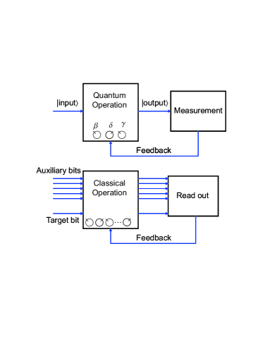
Figure 1: Diagram of classical and quantum learning machines. The learning procedure consists in a sequence of taking the inputs, performing transformations on them, returning the outputs, estimating the figure of merit between the outputs obtained and the expected ones and correspondingly making adjustments to the transformations. For the task of extracting the $k$-th root of NOT (see text for definition) the dimension of the space of parameters for a classical machine is log 2k larger than that for a quantum machine.

Any single qubit rotation can be parameterized by Euler’s angles as follows:

$$U=e^{i\alpha}\left(\begin{array}[]{cc}e^{-i\left(\frac{\beta}{2}+\frac{\delta}{2}\right)}\cos\left(\frac{\gamma}{2}\right)&-e^{i\left(-\frac{\beta}{2}+\frac{\delta}{2}\right)}\sin\left(\frac{\gamma}{2}\right)\\ e^{i\left(\frac{\beta}{2}-\frac{\delta}{2}\right)}\sin\left(\frac{\gamma}{2}\right)&e^{i\left(\frac{\beta}{2}+\frac{\delta}{2}\right)}\cos\left(\frac{\gamma}{2}\right)\\ \end{array}\right).$$ (1)

Since the global phase $\alpha$ is irrelevant for the present application, we are left with the parameters $\delta\in[0,2\pi]$, $\beta\in[0,2\pi]$, $\gamma\in[0,\pi]$. In every new learning trial these parameters will be selected independently with a normal probability distribution centered around the values from the previous run and the widths of the Gaussians are taken as free parameters of the simulation. There are two free parameters of the learning procedure: $\sigma_{\gamma}$ and $\sigma_{\beta}$ ($\sigma_{\delta}=\sigma_{\beta}$). In all simulations these parameters are optimized to minimize the number of learning steps.

Note that if quantum machine performs the task for $n=1$ perfectly, then it will also perform the task perfectly for all $n$. This is why our quantum machine is trained only to learn the task for $n=1$. Nevertheless, after the learning has been completed one should compare how close the performance of the learning machine is to this of the target operation for all $n$. We define a set of figures of merit $\left\{P^{n}\right\}_{n=1}^{\infty}$ as follows:

$$P^{1} = \frac{1}{2}(|\langle 0|U^{k}|1\rangle|^{2}+|\langle 1|U^{k}|0\rangle|^{2})$$ (2)

$$P^{2} = \frac{1}{4}(|\langle 0|U^{k}|1\rangle|^{2}+|\langle 1|U^{k}|0\rangle|^{2}+|\langle 0|U^{2k}|0\rangle|^{2}+\langle 1|U^{2k}|1\rangle|^{2})$$

$$P^{n} = \frac{1}{2n}(|\langle 0|U^{k}|1\rangle|^{2}+|\langle 1|U^{k}|0\rangle|^{2}+$$

$$\dots+|\langle 0|U^{nk}|b\rangle|^{2}+|\langle 1|U^{nk}|b\oplus 1\rangle|^{2}),$$

where $b=0$ if $n$ is even, and $b=1$ if $n$ is odd, and $\oplus$ denotes sum modulo 2. Note that each subsequent $P^{n}$ is more demanding in the sense that more constraints from the definition of the $\sqrt[k]{\mbox{NOT}}$ are being taken into account. This is reflected by the resultsprocedure, which are presented in Fig. 2.

The memory size of the teacher $M$ is another free parameter of the quantum machine. The learning ability has a very strong dependence on $M$ as can be seen from Fig. 3. For lower values of M $M$ the learning is faster at the beginning (up to about 4x$10^{4}$ trials), before it slows down and saturates. At the saturation the size of the memory does not allow distinguishing between sufficiently “good” operations all for which $new_{s}=M$. For higher $M$ values the learning is slower, but it reaches higher fidelities. To combine the high speed with the high fidelity of learning we apply the learning procedure with variable $M$: The machine starts with $M=1$ and whenever it obtains the number of successes $new_{s}=M$ it increments $M$ by one. With this kind of algorithm the learning has one less free parameter. All our simulations were done for variable $M$, unless stated otherwise.

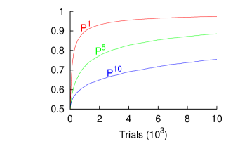
Figure 2: Quantum learning for performing the $4$-th root of NOT. Different figures of merit $P^{s}$ ($s=1,5,10$) as a function of the number of learning trials (x $10^{3}$). The size of teachers memory $M$ is varied to achieve the maximal value of the figures of merits for a given number of trials. The free parameters have the values $\sigma_{\gamma}=\frac{\pi}{4}$ and $\sigma_{\alpha}=\sigma_{\beta}=\frac{\pi}{8}$.

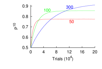
Figure 3: Quantum learning for performing the $4$-th root of NOT. Figure of merit $P^{10}$ as a function of the number of learning trials (x $10^{4})$ for different sizes of teachers memory $M$ (blue = 300, green =100, red=50). The free parameters have the values $\sigma_{\gamma}=\frac{\pi}{4}$ and $\sigma_{\alpha}=\sigma_{\beta}=\frac{\pi}{8}$

Next we describe the classical learning procedure.

Classical learning: The classical learning is an iterative process of finding the optimal probability distribution $p(\vec{i},\vec{j})$ for the classical machine to extract the $\sqrt[k]{\mbox{NOT}}$. The speed of learning depends on the number $N^{2}-N$ of independent parameters (independent probabilities $p(\vec{i},\vec{j})$), where $N=2^{dim(i)}$ and $dim(i)$ is the dimension of the input $\vec{i}$ and the output vector $\vec{j}$. We will refer to $N$ as the memory size of the classical learning machines because it is equal to the total number of distinguishable internal states of the machine. To minimize the number of learning trials required to complete the learning and thus to maximize the speed of learning, we are interested in the minimal number of internal states $N$ for which it is possible to construct a classical machine that is able to extract $\sqrt[k]{\mbox{NOT}}$.

Lemma: Any classical machine that performs $k$-th root of NOT perfectly must have at least $2k$ internal states if $k=2^{m}$ and $m\in\mathbb{N}$.

Proof. Each probabilistic classical machine can be considered as a convex combination of deterministic ones. If it performs some task perfectly, then there must also be deterministic machine that does the same. This means that we can restrict ourselves in this proof only to deterministic machines without any loss of generality. Any (deterministic, classical) machine can be represented as an oriented graph, with vertices corresponding to the internal states. Edge pointing from vertex $\vec{i}$ to $\vec{j}$ will mean that the operation on input $\vec{i}$ generates the output $\vec{j}$. Any (finite) machine must have at least one loop and, if the machine is run subsequently a large number of times, it will eventually end up in that loop. Since the definition of the task involves arbitrary large $n$’s we may start our analysis from $n$ large enough such that the machine is already in the loop. Since we will prove the lemma by giving constraint from below on the size of the loop, we may assume that the whole graph is a one loop and each vertex is a part of it.

Let the length of the loop be $N$. Let $g$ be the greatest common divisor $g=GCD(k,N)$. Then there exist numbers $x$ and $y$ such that

$$k=gx\quad N=gy\quad GCD(x,y)=1$$ (3)

If the machine is initially in a vertex that corresponds to input “1” of the target bit and we apply the operation $Nk$ times we will always end up in the same vertex “1”, since $Nk=0\mod N$. Since, however, the task is defined such that for $N$ odd the ending vertex should correspond to “0” value for the target bit, one concludes that $N$ must be even. Therefore, we can write $N$ as $N=2^{K}c$, where $c$ is odd and $K\geq 1$. We also have $Nx=0\mod N$, but since $Nx=gyx=ky$, then $ky=0\mod N$. According to our definition of $\sqrt[k]{\mbox{NOT}}$ this implies that $y$ is even and, since $GCD(y,x)=1$, $x$ is odd. Also

$$y=\frac{N}{g}=\frac{Nx}{k}=2^{K-m}xc$$ (4)

Since $y$ is even and both $x$ and $c$ odd, then $K\geq m+1$ must hold. We conclude with $N=2^{K}c\geq 2^{K}\geq 2^{m+1}=2k$.

The Lemma implies that if the machine is to perform $\sqrt[k]{\mbox{NOT}}$ perfectly it needs to have $\log k=m$ auxiliary bits in addition to the target bit. It is easy to check that this is not only necessary but also a sufficient condition. One just needs to design machine that is a loop of length $2k$ where the vertices corresponding to initial target input bits 0 and 1 are at a distance $k$ from each other. The number of functions with this property divided by the total number of functions $f:\{0,1\}^{2k}\to\{0,1\}^{2k}$ gives the fraction of the target functions:

$$R=\frac{(2k-4)!(2k-2)(k^{2}-2)}{(2k)^{2k}}\simeq O\left(\frac{1}{k4^{k}}\right).$$ (5)

The target functions thus constitute an exponential small fraction of all functions. Next, we will consider probabilistic classical machines which in order to approximate the target functions with high probability need to be sufficiently “close” (e.g. in the sense of Kullback-Leibler divergence) in the probability space. In such a way both the quantum and classical machines “search” in a continuous space of parameters, however, the relative fraction of this space that is close to the target functions is obviously much larger for the quantum case.

In the case of quantum machine any root of NOT can be performed with only one qubit. The operation that performs $\sqrt[k]{\mbox{NOT}}$ is $\sqrt[k]{\sigma_{x}}$, where $\sigma_{x}$ is spin matrix along direction $x$. Therefore, the memory requirements for our family of problems grows as $\log k$ in the classical case, while remaining constant in the quantum one.

Next, we introduce the classical learning procedure. We assume that the classical machine is initially in a “random” state for which $p(\vec{i},\vec{j})=\frac{1}{2k}.$ The learning process consist of the following steps:

1. Set initially the internal state of the machine such that its first bit (target bit) is in 0 or 1 with equal probability. All auxiliary bits are in 0.

2. Apply the operation $k$ times and after each of them read out the output: $\vec{j}_{r}$, with $r\in\{1,...,k\}$. We observe a sequence $\vec{i}\equiv\vec{j}_{0}\rightarrow\vec{j}_{1}\rightarrow\vec{j}_{2}\rightarrow...\rightarrow\vec{j}_{k}$ of machine’ states. If the target bit of the final state $\vec{j}_{k}$ is inverse of the target bit of initial state $\vec{i}$, move to step 3. Otherwise move to 4.

3. Increase every probability $p(\vec{j}_{r-1},\vec{j}_{r})$ that led to success by adding a factor $1\geq K_{s}\geq 0$. Renormalize the probability distribution such that $\sum_{\vec{j}}p(\vec{i},\vec{j})=1$ and go back to step 2.

4. Decrease every probability $p(\vec{j}_{r-1},\vec{j}_{r})$ that led to a failure by subtracting a factor $1\geq K_{f}\geq 0$ (if then the probability is negative, put it to be 0). Renormalize the probability distribution and go back to step 1.

Note that repeating the steps 2. and 3. the classical machine gradually learns to perform the task for all $n$. The learning has two free parameters $K_{s}$ and $K_{f}$, exactly like the quantum learning (with a variable teachers memory size $M$). To estimate how close is machine’s functioning to the one of the target machine we use the set of figures of merit for all $n$: $\left\{P^{n}\right\}_{n=1}^{\infty}$, which are similar to those of Eq. (2). For example, $P^{2}\equiv P_{k}(0,1)+P_{k}(1,0)+P_{2k}(0,0)+P_{2k}(1,1)$, where $P_{k}(1,0)$ is the probability that the target bit has been changed from 1 to 0 after applying the transformation $k$ times and other probabilities are similarly defined.

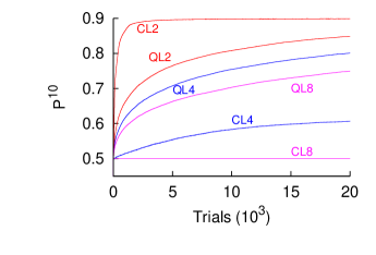
Figure 4: The figure of merit ($P^{10}$) of classical (CL) and quantum (QL) learning for performing different $k$-th ($k=2,4,8$) roots of NOT as a function of the number of learning trials (x$10^{3}$). The values of free parameters are chosen to maximize the figure of merit. Already for $k=4$ quantum learning is faster than the classical one. For the 8-th root of NOT, the figure of merit of classical learning is as for a random choice ($=0.5$) at the given time scale. The free parameters have the values $\sigma_{\gamma}=\frac{\pi}{4}$ and $\sigma_{\alpha}=\sigma_{\beta}=\frac{\pi}{8}$ (for all roots) for the quantum case and the values $K_{s}=K_{f}=0.25$ (2nd root), $K_{s}=K_{f}=0.75$ (4th root) and $K_{s}=0.75\;K_{f}=0.25$ (8th root) for the classical one.

We have performed computer simulations of the both quantum and classical learning process. The results are presented in Fig. 4. We see that the learning in the quantum case is much faster for $k>2$. This speed-up can be understood if one realizes that for the present problem the process of learning is an optimization of a square matrix: unitary transformation $U$ in the quantum case, and a matrix with entries $p(\vec{i},\vec{j})$ in the classical one. While the size of $U$ remains 2 (with complex entries), the size of the matrix with entries $p(\vec{i},\vec{j})$ grows linearly with $k$. It is clear that optimization of significantly larger matrices requires more iterative steps and thus leads to slower learning.

The classical learning algorithm given is not the most general and might not be optimal. The general framework for finding optimal learning procedures is still not fully understood. We have chosen the quantum and classical learning algorithms such that the comparison between them is most evident. The two tasks, i.e. finding a unitary operator for the $k$-th root of NOT, and finding a classical probability distribution that generates the $k$-th root of NOT, though are different from the physical point of view, both require optimization of matrix elements. Since for a given task, the classical machines require a significantly larger number of independent parameters (of which only a small fraction leads to the desired matrix) to be optimized, it is natural to assume that they also require a larger number of learning steps to accomplish learning, regardless of the explicit learning procedure employed. This is exactly what our numerical simulations show.

Quantum information processing has been shown to allow a speed-up over the best possible classical algorithms in computation and has advantages over its classical counterpart in communication tasks, such as secure transmission of information or communication complexity. In this paper we extend the list with a novel task from the field of machine learning: learning to perform the $k$-th root of NOT.

Acknowledgments

We acknowledge support from the EC Project QAP (No. 015848), the Austrian Science Foundation FWF within Projects No. P19570-N16, SFB and CoQuS No. W1210-N16, the Ministerio de Ciencia e Innovación (Fellowship BES-2006-13234) and the Instituto Carlos I for the use of computational resources. The collaboration is a part of an ÖAD/MNiSW program. Č.B. thanks J. Lee for discussions.

References

- (1) M. A. Nielsen and I. L. Chuang, Quantum Computation and Quantum Information (Cambridge University Press, 2000, UK).
- (2) E. Aimeur, G. Brassard, S. Gambs, Canadian Conference on AI 2006 pp 431-442.
- (3) A. Atici, and R.A. Servedio, Quant. Inf. Proc., 4, 355, (2005).
- (4) M. Hunziker, D.A. Meyer, J. Park,J. Pommersheim, and M. Rothstein, arXiv:quant-ph/0309059.
- (5) G. Purushothaman and N. B. Karayiannis, IEEE Trans. Neural Networks, 8:679 (1997).
- (6) E.C. Behrman, L.R. Nash, J.E. Steck, V.G. Chandrashekar and S.R. Skinner. Information Sciences, 128:257 (2000).
- (7) D. G. Fischer, S. H. Kienle, and M. Freyberger, Phys. Rev. A, 61:032306, 2000.
- (8) R. S. Judson and H. Rabitz, Phys. Rev. Lett., 68:1500 (1991).
- (9) T. Baumert, T. Brixner, V. Seyfried, M. Strehle, and G. Gerber, Appl. Phys. B, 65:779 (1997).
- (10) A. Assion, T. Baumert, M. Bergt, T. Brixner, B. Kiefer, V. Seyfried, M. Strehle, and G. Gerber, Science 282:919 (1998).
- (11) R. Neigovzen, J. Neves, R. Sollacher and S. J. Glaser, Phys. Rev. A 79, 042321 (2009).
- (12) M. Sasaki and A. Carlini, Phys. Rev. A 66, 22303 (2002).
- (13) J. Bang, J. Lim, M.S. Kim and J. Lee, arXiv:0803.2976.
- (14) S. Gammelmark and K. Molmer, New J. Phys. 11, 033017 (2009).
- (15) M. Hillery, and V. Buzek, Contemporary Physics 50, 575-586 (2009).