The Omega Effect for Neutral Mesons

Abstract

The possible role of decoherence due to space-time foam is discussed within the context of two models, one based on string/brane theory. and the other based on properties of black hole horizons in general relativity. It is argued that the density matrix satisfies a dissipative master equation, primarily from the study of renormalization group flows  in non-critical string theory.This interpretation of the zero mode of the Liouville field as time leads necessarily to the CPT operator being ill defined. One striking consequence is that the quantum mechanical correlations of pair states of neutral mesons produced in meson factories are changed from the usual EPR state. The magnitude of this departure from EPR correlations is characterised by a parameter $\omega$. The predicted value of $\omega$ is very small or zero. However it is shown explicitly that the the non-vanishing of $\omega$ is only a feature of the model based on string/brane theory.

1 Introduction

The important feature of General Relativity (GR), the classical field theory describing gravity, is the fact that space-time is not simply a frame of coordinates, on which events take place, but is itself a dynamical entity. The quantisation of the theory, poses a problem, given that the coordinates of space-time themselves appear “fuzzy”. The fuzziness of space-time is associated with microscopic quantum fluctuations of the metric field, which may be singular. For instance, one may have Planck size ($10^{-35}$ m) black holes, emerging from the quantum gravity “vacuum”, which may give space-time a “foamy”, topologically non-trivial structure. The semi-classical study of black holes in GR has led to the prediction of Hawking radiation. In classical GR simple solutions for black holes exhibit event horizons. This was interpreted quantum mechanically in terms of lack of communication between Hilbert spaces within and outside the horizon. This is at the basis of the information paradox[1]. Simple arguments relating to tracing over states then lead to a description in terms of non-pure density matrices. These observations have led to a vigorous debate concerning the validity of unitary evolution for quantum gravity. Initially S. Hawking believed that there was information loss; he and others have recently claimed [2] that information is not lost in the presence of a black hole, but rather it is entangled in a holographic way with the portion of space-time outside the horizon. There seems currently more and more adherents to this point of view. However in my opinion the situation is not resolved. This is primarily because we do not have a theory of quantum gravity. Consequently there are always certain loose ends in the arguments that are proposed. As an example the original argument of Hawking has been criticized [3] on the grounds that horizons are mathematical constructs and are not as physically relevant as trapping surfaces. It is then argued that evaporating black holes can evade the information paradox owing to the presence of an inner and outer trapping surface. The recent arguments of Hawking and other (string) theorists are somewhat special in their details and require constructions such as the extremality of black holes, anti-de Sitter (supersymmetric) space-times and the Euclidean formulation for summing over space-time geometries. Such considerations have led to a point of view labelled as holography and black hole complementarity[4],[5] .The special features in these arguments make it hard to make general statements about unitarity or the lack of it in quantum evolution.

We will take a somewhat different point of view which will put us firmly in the camp of those who believe that there is non-unitary evolution due to quantum gravity. Much of the discussion using string theory is based on critical strings where the demands of world sheet conformal and target space Lorentz invariance constrain the allowed values of space-time dimension (see e.g. [6]). Consequently changes in space-time backgrounds cannot be accommodated. Surely a proper theory of quantum gravity needs to be able to handle this. This is a fundamental problem. An approach which takes some steps to address these issues is based on the theory of non-critical strings[7] also referred to as two dimensional gravity coupled to matter. The restoration of conformal invariance for a number of spatial dimensions different from the critical value is addressed through the introduction of the Liouville field. Furthermore by studying the recoil of branes and the induced backreaction on space-time, it possible to consider some situations where the space-time metric and hence geometry is changed. When $p$ space dimensional Dirichlet (Dp) branes are considered, it is no longer necessary to concentrate on the properties of microscopic black holes and the inherent issues of trapped surfaces. In particular Dp branes with $p=0$ exist in some string theories such as bosonic, type IIA and type I. Furthermore even when elementary D particles cannot exist consistently there can be effective D-particles formed by the compactification of higher dimensional D branes. Moreover D particles are non-perturbative constructions since their masses are inversely proportional to the the string coupling ${g_{s}}$ . The introduction of the Liouville field opens up also an interesting possibility. It was suggested by Shore [8] that a renormalization group scale which was local on the world sheet was a useful way of analyzing string theory sigma models (in the sense of the Zamolodchikov C-function) and subsequently [7] this scale was identified with the Liouville field. Furthermore the zero mode of the Liouville field  can be identified with time on the basis of transformation properties of vertex operators associated with D particles [9]. The Zamolodchikov C theorem (for general two dimensional field theories) requires that the C-function (a function in the space of all couplings, i.e. theory space) is a non-negative and non-increasing function on a renormalization group trajectory. The renormalization group trajectory can be identified with temporal evolution as just intimated and this leads, because of the increase of entropy along the trajectories, to a non-unitary evolution for the density matrix $\rho$. It will suffice for us to note that the evolution has the form

$$\frac{{\partial\rho}}{{\partial t}}=i\left[{\rho,H}\right]+\delta\not H\rho\,$$ (1)

where $H$ is the hamiltonian and $\delta\not H\rho$ is formally written as

$$\delta\not H\rho={\beta^{i}}{G_{ij}}\frac{{\partial\rho}}{{\partial{p_{j}}}}.$$ (2)

Here $G_{ij}$ is the so called Zamolodchikov metric, ${\beta^{i}}$ is the renormalization group $\beta$ function for the couplings $g_{i}$ associated with vertex functions $p_{j}$ spanning theory space. Although the identification of the Liouville field with the local renormalization group scale is not rigorous, it is one important feature which influences our joining of the ”non-unitary” camp. The other important reason for us is D-particle recoil which will be addressed in a later section.

The second model to be considered by us is concerned with the effect of horizons and the consequent absence of unitarity but the formulation is not supported by a formal theory like string theory. A different effective theory of space-time foam has been proposed by Garay [10]. The fuzziness of space-time  at the Planck scale is described by a non-fluctuating background which is supplemented by non-local interactions. The latter reflects the fact that at Planck scales space-time points lose their meaning and so these fluctuations present themselves in the non-fluctuating coarse grained background as non-local interactions. These non-local interactions are then rephrased as a quantum thermal bath with a Planckian temperature. The quantum entanglement of the gravitational bath and the two meson (entangled) state is explicit in this model. Consequently issues of back reaction can be readily examined. Since the evolution resulting from the standard Lindblad formulation does not lead to the $\omega$ effect, this manifestation of CPTV is not the result of some arbitrary non-unitary evolution. Hence it is interesting to study the above two quite distinct models (one motivated by string theory and the other by the properties of black holes in general relativity) for clues concerning the appearance of (and an estimate for the order of magnitude) of $\omega$.

Recently these fundamental issues have been brought into sharp focus through a phenomenological analysis involving correlated neutral meson pairs. For equations such as (1), it is well known that initial pure states evolve into mixed ones and so the S-matrix $\not S$ relating initial and final density matrices does not factorise, i.e.

$$\not S\neq SS^{{\dagger}}$$ (3)

where $S=e^{iHt}$. This is another way  of saying that we have  non-unitary evolution. In these circumstances Wald [11] has shown that CPT is violated, at least in its strong form, i.e. there is no unitary invertible operator $\Theta$ such that

$$\Theta\overline{\rho}_{\mathrm{in}}=\rho_{\mathrm{out}}\mathrm{.}$$ (4)

This result is due to the entanglement of the gravitational fluctuations with the matter system.

It was pointed out in [12], that if the CPT operator is not well defined then this has implications for the symmetry structure of the initial entangled state of two neutral mesons in meson factories. Indeed, if CPT can be defined as a quantum mechanical operator, then the decay of a (generic) meson with quantum numbers $J^{PC}=1^{--}$ [13], leads to a pair state of neutral mesons $\left|i\right\rangle$ having the form of the entangled state

$$\left|i\right\rangle=\frac{1}{\sqrt{2}}\left(\left|\overline{M_{0}}\left(\overrightarrow{k}\right)\right\rangle\left|M_{0}\left(-\overrightarrow{k}\right)\right\rangle-\left|M_{0}\left(\overrightarrow{k}\right)\right\rangle\left|\overline{M_{0}}\left(-\overrightarrow{k}\right)\right\rangle\right).$$ (5)

This state has the Bose symmetry associated with particle-antiparticle indistinguishability $C\mathcal{P}=+$, where $C$ is the charge conjugation and $\mathcal{P}$ is the permutation operation. If, however, CPT is not a good symmetry (i.e. ill-defined due to space-time foam), then $M_{0}$ and $\overline{M_{0}}$ may not be identified and the requirement of $C\mathcal{P}=+$ is relaxed [12]. Consequently, in a perturbative framework, the state of the meson pair can be parametrised to have the following form:

$$\left|i\right\rangle=\frac{1}{\sqrt{2}}\left(\left|\overline{M_{0}}\left(\overrightarrow{k}\right)\right\rangle\left|M_{0}\left(-\overrightarrow{k}\right)\right\rangle-\left|M_{0}\left(\overrightarrow{k}\right)\right\rangle\left|\overline{M_{0}}\left(-\overrightarrow{k}\right)\right\rangle\right)\\ +{\frac{\omega}{\sqrt{2}}}\left|{\Delta\left({\vec{k}}\right)}\right\rangle$$

where

$$\left|{\Delta\left({\vec{k}}\right)}\right\rangle\equiv\left|{{{\overline{M}}_{0}}\left({\vec{k}}\right)}\right\rangle\left|{{M_{0}}\left({-\vec{k}}\right)}\right\rangle+\left|{{M_{0}}\left({\vec{k}}\right)}\right\rangle\left|{{{\overline{M}}_{0}}\left({-\vec{k}}\right)}\right\rangle$$

and $\omega=\left|\omega\right|e^{i\Omega}$ is a complex CPT violating (CPTV) parameter. For definiteness in what follows we shall term this quantum-gravity effect in the initial state as the “$\omega$-effect”[12]. There is actually another dynamical “$\omega$-effect” which is generated during the time evolution of the meson pair but this will not be discussed here [14].

The structure of the article will be the following: we commence our analysis by discussing the omega effect.We will then proceed to discuss a string based model for the omega effect. The difficulty of generating the omega effect using other plausible approaches incorporating open systems and non-unitary master equations is illustrated through a class of models which we dub the thermal bath model.

2 D-particles

String theory was found, in the so called first revolution, to contain quantum gravity while in the second revolution the proposal of D(irichlet) brane solitons [15, 16], together with dualities brought about relationships between the different string theories that had been proposed earlier. In particular zero dimensional D-branes [17] occur (in bosonic and some supersymmetric string theories) and are known as D-particles. The spectrum of open strings attached to a Dp brane (with $p>0$ ) contains a Maxwell field and the ends of the open string carry charge. The associated Maxwell field is confined to the world volume of the D brane. Hence a conventionally charged string cannot end on a D-particle. We will thus restrict our consideration to neutral particles that are ”captured”  by D-particles. The D-particle solitons are fundamental scalar particles in the dual theories. Interactions in string theory are, as yet, not treated as systematically as in ordinary quantum field theory where a second quantised formalism is defined. The latter leads in a systematic way to the standard formulations by Schwinger and Feynman of perturbation series. When we consider stringy matter interacting with other matter or D-particles, the world lines traced out by point particles are replaced by two-dimensional world sheets. World sheets are the parameter space of the first quantised operators ( fermionic or bosonic) representing strings. In this way the first quantised string is represented by actually a two dimensional (world-sheet) quantum field theory. An important symmetry of this first quantised string theory is conformal invariance and the requirement of the latter does determine the space-time dimension and/or structure.  This symmetry leads to a scaling of the metric and permits the representation of interactions through the construction of measures on inequivalent Riemann surfaces [18]. In and out states of stringy matter are represented by punctures at the boundaries. The D-particles as solitonic states [16] in string theory do fluctuate themselves, and this is described by stringy excitations, corresponding to open strings with their ends attached to the D-particles. In the first quantised (world-sheet) language, such fluctuations are also described by Riemann surfaces of higher topology with appropriate Dirichlet boundary conditions (c.f. fig. 1). The plethora of Feynman diagrams in higher order quantum field theory is replaced by a small set of world sheet diagrams classified by moduli which need to be summed or integrated over [6].

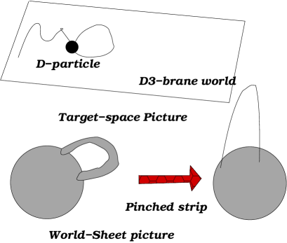
Figure 1: Upper picture: A Fluctuating D-particle is described by open strings attached to it. As a result of conservation of fluxes [15, 16, 17] that accompany the D-branes, an isolated D-particle cannot occur, but it has to be connected to a D-brane world through flux strings. Lower picture: World-sheet diagrams with annulus topologies, describing the fluctuations of D-particles as a result of the open string states ending on them. Conformal invariance implies that pinched surfaces, with infinitely long thin strips, have to be taken into account. In bosonic string theory, such surfaces can be resummed [22].

In order to understand possible consequences for CPT due to space-time foam we will have to characterise the latter. The model we will consider is based on D-particles populating a bulk geometry between parallel D-brane worlds. The model is termed D-foam [19] (c.f. figure 2), since our world is modelled as a three-brane moving in the bulk geometry. As a result, D-particles cross the brane world, and thereby appear as foamy flashing on and off structures for an observer on the brane.

Figure 2: Schematic representation of a D-foam. The figure indicates also the capture/recoil process of a string state by a D-particle defect for closed (left) and open (right) string states, in the presence of D-brane world. The presence of a D-brane is essential due to gauge flux conservation, since an isolated D-particle cannot exist. The intermediate composite state at $t=0$, which has a life time within the stringy uncertainty time interval $\delta t$, of the order of the string length, and is described by world-sheet logarithmic conformal field theory, is responsible for the distortion of the surrounding space time during the scattering, and subsequently leads to induced metrics depending on both coordinates and momenta of the string state. This results on modified dispersion relations for the open string propagation in such a situation [19], leading to non-trivial “optics” for this space time.

Even at low energies $E$, such a foam may have observable consequences e.g. decoherence  effects which may be of magnitude $O\left(\left[\frac{E}{M_{P}}\right]^{n}\right)$ with $n=1,2$ where $M_{P}$ is the Planck mass or change in the usual Lorentz invariant dispersion relations.The study of D-brane dynamics has been made possible by Polchinski’s realisation that such solitonic string backgrounds can be described in a conformally invariant way in terms of world sheets with boundaries [16]. On these boundaries Dirichlet boundary conditions for the collective target-space coordinates of the soliton are imposed [20]. Heuristically, when low energy matter given by a closed string propagating in a $\left(d+1\right)$-dimensional space-time collides with a very massive D-particle (0-brane) embedded in this space-time, the D-particle recoils as a result [21]. We shall consider the simple case of bosonic stringy matter coupling to D-particles and so we can only discuss matters of principle and ignore issues of stability. However we should note that an open string model needs to incorporate for completeness, higher dimensional D-branes such as the D3 brane. This is due to the vectorial charge carried by the string owing to the Kalb-Ramond field. Higher dimensional D-branes (unlike D-particles) can carry the charge from the endpoints of open strings that are attached to them. For a closed bosonic string model the inclusion of such D-branes is not imperative (see figure 2). The higher dimensional branes are not pertinent to our analysis however. The current state of phenomenolgical modelling of the interactions of D-particle foam with stringy matter will be briefly summarised now. Since there are no rigid bodies in general relativity the recoil fluctuations of the brane and their effective stochastic back-reaction on space-time cannot be neglected. As we will discuss, D-particle recoil in the ”tree approximation” i.e. in lowest order in the string coupling $g_{s}$, corresponds to the punctured disc or Riemann sphere approximation in open or closed string theory, induces a non-trivial space-time metric. For closed strings colliding with a heavy (non-relativistic) D-particle the metric has the form [23]

$$g_{ij}=\delta_{ij},\,g_{00}=-1,g_{0i}=\varepsilon\left(\varepsilon y_{i}+u_{i}t\right)\Theta_{\varepsilon}\left(t\right),\;i=1,\ldots,d.$$ (6)

Here the suffix $0$ denotes temporal (Liouville) components, $\frac{u_{i}}{\varepsilon}\propto g_{s}\frac{\Delta k_{i}}{M_{s}}$, where $\Delta k_{i}=\left(k_{1}-k_{2}\right)_{i}$ and $k_{1}\left(k_{2}\right)$ is the momentum of the propagating closed-string state before (after) the recoil, $y_{i}$ are the spatial collective coordinates of the D- particle and $\varepsilon^{-2}$ is identified with the target Minkowski time $t$ for $t\gg 0$ after the collision; $\Theta_{\varepsilon}\left(t\right)$ is the regularised step function represented by

$$\Theta_{\varepsilon}\left(t\right)=\frac{1}{2\pi i}\int_{-\infty}^{\infty}\frac{dq}{q-i\varepsilon}e^{iqt},$$ (7)

and $u_{i}$ is small,. For our purposes the Liouville and Minkowski times can be identified. Now for large $t,$ to leading order,

$$g_{0i}\simeq\overline{u}_{i}\equiv\frac{u_{i}}{\varepsilon}$$ (8)

where $\Delta p_{i}$ is the momentum transfer during a collision and $M_{s}$ is the string mass scale, $g_{s}<1$ is the string coupling, assumed weak, and the combination $M_{s}/g_{s}$ is the D-particle mass, playing the rôle of the Quantum Gravity scale in this problem, i.e. the Planck mass; this formalism has been used to establish a phenomenological model where the couplings $u_{i}$ are taken to be stochastic and modeled by a gaussian process[24]. The stochasticity is due to two contributions. The D-particle has an initial random recoil velocity due to capture of stringy matter and subsequent release. Furthermore sumperimposed on this randomness are quantum fluctuations due to vacuum string excitations.The process of capture and emission does not have to conserve flavour. Consequently we need to generalise the stochastic structure to allow for this.The fluctuations of each component of the metric tensor $g^{\alpha\beta}$ will then not be just given by the simple recoil distortion (6), but instead will be taken to have a $2\times 2$ (“flavour”) structure [14]:

$${g^{00}} = \left({-1+{r_{4}}}\right)\underline{\underline{1}}$$

$${g^{01}} = {g^{10}}={r_{0}}\underline{\underline{1}}+{r_{1}}{\sigma_{1}}+{r_{2}}{\sigma_{2}}+{r_{3}}{\sigma_{3}}$$

$${g^{11}} = \left({1+{r_{5}}}\right)\underline{\underline{1}}$$ (9)

where $\underline{\underline{1}}$ , is the identity operator and $\sigma_{i}$ are the Pauli matrices and the $r_{\mu}$ are random variables which obey

$$\left\langle r_{\mu}\right\rangle=0,\;\left\langle r_{\mu}r_{\nu}\right\rangle=\Delta_{\mu}\delta_{\mu\nu}.$$ (10)

The above parametrisation has been taken for simplicity and also we will consider motion to be in the $x$- direction which is natural since the meson pairs move collinearly. The above parametrisation has been taken for simplicity and we will also consider motion to be in the $x$- direction which is natural since the meson pairs move collinearly. In any given realisation of the random variables for a gravitational background, the system evolution can be considered to be given by the Klein-Gordon equation for a two component spinless neutral meson field $\Phi=\left(\begin{array}[c]{c}\phi_{1}\\ \phi_{2}\end{array}\right)$ (corresponding to the two flavours) with mass matrix $m=\frac{1}{2}\left(m_{1}+m_{2}\right)\underline{\underline{1}}+\frac{1}{2}\left(m_{1}-m_{2}\right)\sigma_{3}$. We thus have

$$(g^{\alpha\beta}D_{\alpha}D_{\beta}-m^{2})\Phi=0$$ (11)

where $D_{\alpha}$ is the covariant derivative. Since the Christoffel symbols vanish (as the $a_{i}$ are independent of space-time) the $D_{\alpha}$ coincide with $\partial_{\alpha}$. Hence within this flavour changing background (11) becomes

$$\left(g^{00}\partial_{0}^{2}+2g^{01}\partial_{0}\partial_{1}+g^{11}\partial_{1}^{2}\right)\Phi-m^{2}\Phi=0.$$ (12)

We shall consider the two particle tensor product states made from the single particle states $\left|\uparrow^{\left(i\right)}\right\rangle$ and $\left|\downarrow^{\left(i\right)}\right\rangle$ $i=1,2$. This includes the correlated states which include the state of the $\omega$ effect. In view of (12) the evolution of this state is governed by a hamiltonian $\widehat{H}$

$$\widehat{H}=g^{01}\left(g^{00}\right)^{-1}\widehat{k}-\left(g^{00}\right)^{-1}\sqrt{\left(g^{01}\right)^{2}{k}^{2}-g^{00}\left(g^{11}k^{2}+m^{2}\right)}$$ (13)

which is the natural generalisation of the standard Klein Gordon hamiltonian in a one particle situation where $\widehat{k}\left|\pm k,\alpha\right\rangle=\pm k\left|\pm k,\alpha\right\rangle$ with $\alpha=\uparrow$ or $\downarrow$. $\widehat{H}$ is a single particle hamiltonian and in order to study two particle states associated with $i=1,2$ we can define $\widehat{H}_{i}$ in the natural way (in terms of $\widehat{H}$) and then the total hamiltonian is $\mathcal{H}=\sum_{i=1}^{2}$ $\widehat{H}_{i}$. The effect of space-time foam on the initial entangled state of two neutral mesons is conceptually difficult to isolate, given that the meson state is itself entangled with the bath. Nevertheless, in the context of our specific model, which is written as a stochastic hamiltonian, one can estimate the order of the associated $\omega$-effect of [14] by applying non-degenerate perturbation theory to the states $\left|\uparrow^{\left(i\right)}\right\rangle$, $\left|\downarrow^{\left(i\right)}\right\rangle$, $i=1,2$ (where the label $\pm k$ is redundant since $i$ already determines it). Although it would be more rigorous to consider the corresponding density matrices, traced over the unobserved gravitational degrees of freedom, in order to obtain estimates it will suffice formally to work with single-meson state vectors .

Owing to the form of the hamiltonian (13) the gravitationally perturbed states will still be momentum eigenstates. The dominant features of a possible $\omega$-effect can be seen from a term $\widehat{H_{I}}$ in the interaction hamiltonian

$$\widehat{H_{I}}=-\left({r_{1}\sigma_{1}+r_{2}\sigma_{2}}\right)\widehat{k}$$ (14)

which is the leading order contribution in the small parameters $r_{i}$ (c.f. (9),(13)) in $H$ (i.e $\sqrt{\Delta_{i}}$ are small). In first order non-degenerate perturbation theory the gravitational dressing of $\left|{\downarrow}^{\left(i\right)}\right\rangle$ leads to a state:

$$\left|\downarrow^{\left(i\right)}\right\rangle_{QG}=\left|\downarrow^{\left(i\right)}\right\rangle+\left|\uparrow^{\left(i\right)}\right\rangle\alpha^{\left(i\right)}$$ (15)

where

$$\alpha^{\left(i\right)}=\frac{\left\langle\uparrow^{\left(i\right)}\right|\widehat{H_{I}}\left|\downarrow^{\left(i\right)}\right\rangle}{E_{2}-E_{1}}$$ (16)

and correspondingly for $\left|{\uparrow}^{\left(i\right)}\right\rangle$ the dressed state is obtained from (16) by $\left|\downarrow\right\rangle\leftrightarrow\left|\uparrow\right\rangle$ and $\alpha\rightarrow\beta$ where

$$\beta^{\left(i\right)}=\frac{\left\langle\downarrow^{\left(i\right)}\right|\widehat{H_{I}}\left|\uparrow^{\left(i\right)}\right\rangle}{E_{1}-E_{2}}$$ (17)

Here the quantities $E_{i}=(m_{i}^{2}+k^{2})^{1/2}$ denote the energy eigenvalues, and $i=1$ is associated with the up state and $i=2$ with the down state. With this in mind the totally antisymmetric “gravitationally-dressed” state can be expressed in terms of the unperturbed single-particle states as:

$$\begin{array}[c]{l}\left|{\uparrow}^{\left(1\right)}\right\rangle_{QG}\left|{\downarrow}^{\left(2\right)}\right\rangle_{QG}-\left|{\downarrow}^{\left(1\right)}\right\rangle_{QG}\left|{\uparrow}^{\left(2\right)}\right\rangle_{QG}=\\ \left|{\uparrow}^{\left(1\right)}\right\rangle\left|{\downarrow}\right\rangle^{\left(2\right)}-\left|{\downarrow}\right\rangle^{\left(1\right)}\left|{\uparrow}\right\rangle^{\left(2\right)}\\ +\left|{\downarrow}^{\left(1\right)}\right\rangle\left|{\downarrow}^{\left(2\right)}\right\rangle\left({\beta^{\left(1\right)}-\beta^{\left(2\right)}}\right)+\left|{\uparrow}^{\left(1\right)}\right\rangle\left|{\uparrow}^{\left(2\right)}\right\rangle\left({\alpha^{\left(2\right)}-\alpha^{\left(1\right)}}\right)\\ +\beta^{\left(1\right)}\alpha^{\left(2\right)}\left|{\downarrow}^{\left(1\right)}\right\rangle\left|{\uparrow}^{\left(2\right)}\right\rangle-\alpha^{\left(1\right)}\beta^{\left(2\right)}\left|{\uparrow}^{\left(1\right)}\right\rangle\left|{\downarrow}^{\left(2\right)}\right\rangle\\ \end{array}$$ (18)

It should be noted that for $r_{i}\propto\delta_{i1}$ the generated $\omega$-like effect corresponds to the case $\alpha^{\left(i\right)}=-\beta^{\left(i\right)}$, while the $\omega$-effect of [25] (5) corresponds to $r_{i}\propto\delta_{i2}$ (and $\alpha^{\left(i\right)}=\beta^{\left(i\right)}$). The velocity recoil $u$ is given by

$$u\sim r$$

and so the variance $\Delta$ can be determined once the variance of $u$ is known. In the perturbative approach we do not need to specify the higher order moments provided they are finite and small. Rigour would demand a density matrix approach but in order to estimate the order of the effect it suffices to note that

$$O\left(\left|\omega^{2}\right|\right)\sim\left\langle\left|{\beta^{\left(1\right)}-\beta^{\left(2\right)}}\right|^{2}\right\rangle$$ (19)

which is an estimate for $|\omega|^{2}$. It is necessary to examine the moments for $u$.

3 A string theory estimate for the variance of the D-particle

In order to estimate the variance of the recoil velcoity we need to understand the dynamics of D-particle foam. It is imperative to consider D-particle quantisation and in particular D-particle recoil as a result of scattering off stringy matter. The issue of recoil is not fully understood and it is not our purpose here to delve into the subtleties of recoil and operators describing recoil. We will rather proceed on the basis of a proposal which has had some success in the past [21]. The energy of a D-particle is independent of its position. Consequently in bosonic string theory there are 25 zero modes, the Dirichlet directions. Zero modes lead to infrared divergences in loops in a field theory setting where collective co-ordinates are used to isolate these infrared divergences. This is essentially due to the naivety of the perturbation series that is used and can be addressed using a coherent state formalism. The situation is similar but, in some ways, worse for string theory since the second quantised formalism for strings is more rudimentary. In string theory the use of first quantisation requires a sum over Riemann sheets with different moduli parameters. The formal transition from one surface to another of lower genus (within string perturbation theory ) has singularities associated with infrared divergences in the integration over moduli parameters. In the case of a disc $D$ an incipient annulus $\Sigma$ can be found by making two punctures and attaching a long thin strip (somewhat like the strap in a handbag and dubbed wormholes). In the limit of vanishing width this wormhole, is represented by a region in moduli space, integration over which leads to an infrared divergence. A similar argument would apply to a Riemann sphere where two punctures would be connected by a long thin tube. For the disc the divergence will be due to propagation of zero mode open string state while for the Riemann sphere it would be an analogous closed string state along the wormhole. Let us examine this divergence explicitly. Consider the correlation function $\left\langle V_{1}V_{2}V_{3}\ldots V_{n}\right\rangle_{\Sigma}$ for vertex operators [18] $\left\{V_{i}\right\}_{i=1,\ldots,n}$ where $\Sigma$ is the Riemann surface of an annulus; it can be deformed into a disc with a wormhole attached [20],[22]. The set of vertex operators include necessarily any higher dimensional D-branes necessary to conserve string charge. However such vertex insertions clearly do not affect the infrared divergence caused by  wormwholes. The correlation function can be expressed as

$$\left\langle V_{1}V_{2}V_{3}\ldots V_{n}\right\rangle_{\Sigma}=\sum_{a}\int{\mathrm{{d}}s_{1}}\int{\mathrm{{d}}s_{2}}\int\frac{\mathrm{d}q}{q}q^{h_{a}-1}\left\langle\phi_{a}\left(s_{1}\right)\phi_{a}\left(s_{2}\right)V_{1}V_{2}V_{3}\ldots V_{n}\right\rangle_{D}$$ (20)

where $s_{1}$ and $s_{2}$ are the positions of the punctures on $\partial D$.The $\left\{\phi_{a}\right\}$ are a complete set of eigenstates of the Virasoro operator $L_{0}$ with conformal weights $h_{a}$[26] and $q$ is a Teichmuller parameter associated with the added thin strip. Clearly there is a potential divergence associated with its disappearance $q\rightarrow 0$ and this corresponds to a long thin strip attached to the disc. For a static D-particle the string co-ordinates $\overrightarrow{X}_{D}=\left\{X^{1},X^{2},X^{3},\ldots,X^{25}\right\}$ have Dirichlet boundary conditions while $X^{0}$ has Neumann boundary conditions (in the static gauge)

$$\left.\frac{\partial}{\partial\sigma}X^{0}\left(\tau,\sigma\right)\right|_{\sigma=0}=0=\left.\frac{\partial}{\partial\sigma}X^{0}\left(\tau,\sigma\right)\right|_{\sigma=\pi}$$ (21)

where $\left(\tau,\sigma\right)$ is a co-ordinisation of the worldsheet.The associated translational zero mode is given by

$$\phi^{i}\left(X,\omega\right)=\frac{\sqrt{g_{s}}}{4}\partial_{n}X_{D}^{i}\e^{i\omega X^{0}},$$ (22)

where $\partial_{n}$ denotes a derivative in the $X^{i}$ Dirichlet direction, and is an element of the set $\left\{\phi_{a}\right\}$. The conformal weight $h_{i}=1+\alpha^{\prime}\omega^{2}$. The relevant part of the integral in (20) is

$$\int_{0}^{1}dq\int_{-\infty}^{\infty}d\omega\,q^{-1+\alpha^{\prime}\omega^{2}}=\int_{0}^{1}dq\,\frac{1}{q\left(-\log q\right)^{1/2}}$$ (23)

and is divergent because of the behaviour of the integrand near $q=0.$ This can be regularized by putting a lower cut-off $q>\delta\rightarrow 0$ in the integral.The correlation function on $\Sigma$ can be computed to be [20]

$$\left\langle V_{1}V_{2}V_{3}\ldots V_{n}\right\rangle_{\Sigma}=-\frac{g_{s}}{16T}\log\delta\left\langle\partial_{n}\overrightarrow{X}_{D}\left(s_{1}\right).\partial_{n}\overrightarrow{X}_{D}\left(s_{2}\right)V_{1}V_{2}V_{3}\ldots V_{n}\right\rangle_{D}$$ (24)

where $T$ is a cut-off for large (target) time. Division by it removes divergencies due to the integration over the world-sheet zero modes of the target time. These should not be confused with divergencies associated with pinched world-sheet surfaces, proportional to $\mathrm{log}\delta$, that we are interested in here. These latter divergences cause conventional conformal invariance to fail.

However, in one approach, it was argued sometime ago, that these divergences can be canceled if D-particles are allowed to recoil [21, 22], as a result of momentum conservation during their scattering with string states. In fact, in our D-particle foam model [19], this is not a simple scattering process, as it involves capture and re-emission of the string state by the D-particle defect. In simple terms, this process involves splitting of strings by the defect. In a world-sheet (first quantization) framework, such processes are described by appropriate vertex operators, whose operator product expansion close on a (local) logarithmic algebra [21, 22]. The translational zero modes are associated with infinitesimal translations in the Dirichlet directions. Given that D-particles do not have any internal or rotational degrees of freedom, these modes should give us valuable information concerning recoil. Moreover (for $\omega=0$) there is a degeneracy in the conformal weights between $\phi^{i}$, $\partial_{\omega}\phi^{i}$ and the identity operator and also the conformal blocks in the corresponding algebra have logarithmic terms.

To understand the formal structure of the world-sheet deformation operators pertinent to the recoil/capture process, we first notice that the world-sheet boundary operator ${V_{D}}$ describing the excitations of a moving heavy D0-brane is given in the tree approximation by:

$${V_{D}}=\int\limits_{\partial D}{\left({{y_{i}}{\partial_{n}}{X^{i}}+{u_{i}}{X^{0}}{\partial_{n}}{X^{i}}}\right)\equiv\int\limits_{\partial D}{{Y_{i}}\left({{X^{0}}}\right){\partial_{n}}{X^{i}}}}$$

where $u_{i}$ and $y_{i}$ are the velocity  and position of the D-particle respectively and $Y_{i}\left(X^{0}\right)\equiv y_{i}+u_{i}X^{0}$. To describe the capture/recoil we need an operator which has non-zero matrix elements between different states of  the D-particle and is turned on “abruptly” in target time. One way of doing this is to put [21] a $\Theta\left(X^{0}\right)$, the Heavyside function, in front of ${V_{D}}$ which models an impulse whereby the D-particle starts moving at $X^{0}=0$. Using Gauss’s theorem this impulsive ${V_{D}}$, denoted by ${V_{D}}^{imp}$, can be represented as

$${V_{D}}^{imp}=\sum_{i=1}^{25}\int_{D}d^{2}z\,\partial_{\alpha}\left(\left[u_{i}X^{0}\right]\Theta\left(X^{0}\right)\partial^{\alpha}X^{i}\right)=\sum_{i=1}^{25}\int_{\partial D}d\tau\,u_{i}X^{0}\Theta\left(X^{0}\right)\partial_{n}X^{i}.$$ (25)

Since $X^{0}$ is an operator it will be necessary to define $\Theta\left(X^{0}\right)$ as an operator using the contour integral

$$\Theta_{\varepsilon}\left(X^{0}\right)=-\frac{i}{2\pi}\int_{-\infty}^{\infty}\frac{d\omega}{\omega-i\varepsilon}\e^{i\omega X^{0}}$$ (26)

with $\varepsilon\rightarrow 0+$.

Hence we can consider

$$D_{\varepsilon}(X^{0})\equiv D(X^{0};\varepsilon)=X^{0}\Theta_{\varepsilon}\left(X^{0}\right)=-\int_{-\infty}^{\infty}\frac{d\omega}{\left(\omega-i\varepsilon\right)^{2}}\e^{i\omega X^{0}}~{}.$$ (27)

The introduction of the feature of impulse in the operator breaks conventional conformal symmetry, but a modified logarithmic conformal algebra holds. A generic logarithmic algebra in terms of operators $\mathcal{C}$ and $\mathcal{D}$ and the stress tensor $T\left(z\right)$ (in complex tensor notation ) satisfies the operator product expansion

$$\begin{array}[]{l}T\left(z\right)C\left({w,\overline{w}}\right)\sim\frac{\Delta}{{{{\left({z-w}\right)}^{2}}}}C\left({w,\overline{w}}\right)+\frac{{\partial C\left({w,\overline{w}}\right)}}{{{{\left({z-w}\right)}^{2}}}}+\cdots\\ T\left(z\right)D\left({w,\overline{w}}\right)\sim\frac{\Delta}{{{{\left({z-w}\right)}^{2}}}}D\left({w,\overline{w}}\right)+\frac{1}{{{{\left({z-w}\right)}^{2}}}}C\left({w,\overline{w}}\right)+\frac{{\partial D\left({w,\overline{w}}\right)}}{{{{\left({z-w}\right)}^{2}}}}+\cdots\\ \end{array}$$

and

$$\left\langle{C\left({z,\overline{z}}\right)C\left({0,0}\right)}\right\rangle \sim 0,$$ (28)

$$\left\langle{C\left({z,\overline{z}}\right)D\left({0,0}\right)}\right\rangle \sim \frac{c}{{{{\left|z\right|}^{2\Delta}}}},$$ (29)

$$\left\langle{D\left({z,\overline{z}}\right)D\left({0,0}\right)}\right\rangle \sim \frac{c}{{{{\left|z\right|}^{2\Delta}}}}\left({\log\left|z\right|+d}\right),$$ (30)

where $d$ is a constant. Since the conformal dimension of $\e^{iqX^{0}}$ is $\frac{q^{2}}{2}$ we find that

$$T\left(w\right)D_{\varepsilon}\left(z\right)\sim-\frac{\varepsilon^{2}}{2\left(w-z\right)^{2}}D_{\varepsilon}\left(z\right)+\frac{1}{\left(w-z\right)^{2}}\varepsilon\Theta_{\varepsilon}\left(X^{0}\right)+\cdots$$ (31)

and so a logarithmic conformal algebra structure arises if we define

$$C_{\varepsilon}(X^{0})\equiv C(X^{0};\varepsilon)=\varepsilon\Theta_{\varepsilon}\left(X^{0}\right)~{},$$ (32)

suppressing, for simplicity, the non-holomorphic piece. The above logarithmic conformal field theory structure is found with this identification. Similarly we find

$$T\left(w\right)C_{\varepsilon}\left(z\right)\sim-\frac{\varepsilon^{2}}{2\left(w-z\right)^{2}}C_{\varepsilon}\left(z\right)+\cdots$$

Consequently $\Delta$ for $C_{\varepsilon}\left(z\right)$ and $D_{\varepsilon}\left(z\right)$ is $-\frac{\varepsilon^{2}}{2}$. A calculation (in a euclidean metric) for a disc of size $L$ with a short-distance worldsheet cut-off $a$ reveals that as $\varepsilon\rightarrow 0$

$$\left\langle{{C_{\varepsilon}}\left({z,\overline{z}}\right){C_{\varepsilon}}\left({0,0}\right)}\right\rangle \sim O\left({{\varepsilon^{2}}}\right),$$ (33)

$$\left\langle{{C_{\varepsilon}}\left({z,\overline{z}}\right){D_{\varepsilon}}\left({0,0}\right)}\right\rangle \sim \frac{\pi}{2}\sqrt{\frac{\pi}{{{\varepsilon^{2}}\alpha}}}\left({1-4{\varepsilon^{2}}\log\left|{\frac{z}{a}}\right|}\right),$$ (34)

$$\left\langle{{D_{\varepsilon}}\left({z,\overline{z}}\right){D_{\varepsilon}}\left({0,0}\right)}\right\rangle \sim \frac{\pi}{2}\sqrt{\frac{\pi}{{{\varepsilon^{2}}\alpha}}}\left({\frac{1}{{{\varepsilon^{2}}}}-4\log\left|{\frac{z}{a}}\right|}\right),$$ (35)

where $\alpha=\log\left|\frac{L}{a}\right|^{2}$. We consider $\varepsilon\rightarrow 0+$ such that

$$\varepsilon^{2}\alpha\sim\frac{1}{2\eta}=O\left(1\right)~{},$$ (36)

where $\eta$ is the time signature and the right-hand side is kept fixed as the cutoff runs; it is then straightforward to see that (33), (34), and (35) are consistent with (28), (29), and (30). It is only under the condition (36) that the recoil operators $C_{\varepsilon}$ and $D_{\varepsilon}$ obey a closed logarithmic conformal algebra [21]:

$$\left\langle{{C_{\varepsilon}}\left(z\right){C_{\varepsilon}}\left(0\right)}\right\rangle \sim 0$$ (37)

$$\left\langle{{C_{\varepsilon}}\left(z\right){D_{\varepsilon}}\left(0\right)}\right\rangle \sim 1$$ (38)

$$\left\langle{{D_{\varepsilon}}\left(z\right){D_{\varepsilon}}\left(0\right)}\right\rangle \sim -4\eta\log\left|{\frac{z}{L}}\right|$$ (39)

The reader should notice that the full recoil operators, involving $\partial_{n}X^{i}$ holomorphic pieces with the conformal-dimension-one entering (25)), obey the full logarithmic algebra (28), (29), (30) with conformal dimensions $\Delta=1-\frac{\varepsilon^{2}}{2}$. From now on we shall adopt the euclidean signature $\eta=1$.

We next remark that, at tree level in the string perturbation sense, the stringy sigma model (inclusive of the D-particle  boundary term and other  vertex operators) is a two dimensional renormalizable quantum field theory; hence for generic couplings $g^{i}$ it is possible to see how the couplings run in the renormalization group sense with changes in the short distance cut-off through the beta functions $\beta^{i}$. In the world-sheet renormalization group [27], based on expansions in powers of the couplings, $\beta^{i}$ has the form ( with no summation over the repeated indices)

$$\beta^{i}=y_{i}g^{i}+\ldots$$ (40)

where $y_{i}$ is the anomalous dimension, which is related to the conformal dimension $\Delta_{i}$ by $y_{i}=\Delta_{i}-\delta$, with $\delta$ the engineering dimension (for the holomorphic parts of vertex operators for the open string $\delta=1$). The $\ldots$ in (40) denote higher orders in $g^{i}$. Consequently, in our case, we note that the (renormalised) D-particle recoil velocities $u^{i}$ constitute such $\sigma$-model couplings, and to lowest order in the renormalised coupling $u_{i}$ the corresponding $\beta$ function satisfies

$$\frac{du^{i}}{d\log\Lambda}=-\frac{\varepsilon^{2}}{2}u^{i}.$$ (41)

where $\Lambda$ is a (covariant) world-sheet renormalization-group scale. In our notation, we identify the logarithm of this scale with $\alpha=\log\left|\frac{L}{a}\right|^{2}$, satisfying (36).

An important comment is now in order concerning the interpretation of the flow of this world-sheet renormalization group scale as a target-time flow. The target time $t$ is identified through $t=2\log\Lambda$. For completeness we recapitulate the arguments of [21] leading to such a conclusion. Let one make a scale transformation on the size of the world-sheet

$$L\rightarrow L^{\prime}=\e^{t/4}L$$ (42)

which is a finite-size scaling (the only one which has physical sense for the open string world-sheet). Because of the relation between $\varepsilon$ and $L$ (36) this transformation will induce a change in $\varepsilon$

$$\varepsilon^{2}\rightarrow\varepsilon^{\prime 2}=\frac{\varepsilon^{2}}{1+\varepsilon^{2}t}$$ (43)

(note that if $\varepsilon$ is infinitesimally small, so is $\varepsilon^{\prime}$ for any finite $t$). From the scale dependence of the correlation functions (39) that $C_{\varepsilon}$ and $D_{\varepsilon}$ transform as ${C_{\varepsilon}}\to{C_{\varepsilon^{\prime}}}={C_{\varepsilon}}$ and ${D_{\varepsilon}}\to{D_{\varepsilon^{\prime}}}={D_{\varepsilon}}+t{C_{\varepsilon}}$.

Hence the coupling constants in front of $C_{\varepsilon}$ and $D_{\varepsilon}$ in the recoil operator (3), i.e. the velocities $u_{i}$ and spatial collective coordinates $y_{i}$ of the brane, must transform like:

$$u_{i}\rightarrow u_{i}~{}~{},~{}~{}y_{i}\rightarrow y_{i}+u_{i}t$$ (44)

This is nothing other than the Galilean transformation for the heavy D-particles and thus it demonstrates that the finite size scaling parameter $t$, entering (42), plays the rôle of target time, on account of (36). Notice that (44) is derived upon using (39), that is in the limit where $\varepsilon\rightarrow 0$. This will become important later on, where we shall discuss (stochastic) relaxation phenomena in our recoiling D-particle.

Thus, in the presence of recoil a world-sheet scale transformation leads to an evolution of the $D$-brane in target space, and from now on we identify the world-sheet renormalization group scale with the target time $t$. In this sense, equation (41) is an evolution equation in target time.

However, this equation does not capture quantum-fluctuation aspects of $u^{i}$ about its classical trajectory with time $u_{i}(t)$. Going to higher orders in perturbation theory of the quantum field theory at fixed genus does not qualitatively alter the situation in the sense that the equation remains deterministic. However the effect of string perturbation theory where higher genus surfaces are considered and re-summed in some appropriate limits can be shown to give rise to quantum fluctuations in $u^{i}$ [28] which leads to a Langevin equation [29] rather than (41). The equation has the form

$$\frac{d{\bar{u}}^{i}}{dt}=-\frac{1}{4t}{\bar{u}}^{i}\,+\frac{g_{s}}{\sqrt{2\alpha^{\prime}}}t^{1/2}\xi\left(t\right)$$ (45)

where $t=\varepsilon^{-2}$ and $\xi\left(t\right)$ represents white noise. This equation is valid for large $t$. From the above analysis it is known that [22] (c.f. Appendix A)) that to $O\left(g_{s}^{2}\right)$ the correlation for $\xi\left(t\right)$ is $\bar{u}^{i}$ independent,  and for time scales of interest, is correlated like white noise ; hence the correlation of $\xi\left(t\right)$ has the form:

$$\left\langle\xi\left(t\right)\xi\left(t^{\prime}\right)\right\rangle=\delta\left(t-t^{\prime}\right).$$ (46)

Since the vectorial nature of $\bar{u}^{i}$ is not crucial for our analysis, we will suppress it and consider the single variable $\bar{u}$. Moreover the mean of $\bar{u}$ vanishes.

4 Langevin equations and fluctuating string coupling

It is possible to solve [28] the Langevin equation (45) (with (46)).The quantity of interest which is an important input for our estimate of the omega effect is the variance of $u$ the velocity of the D-particle. If the D-particle is typically interacting with matter on a time scale of $t_{0}$, then the effect of a large number of such collisions can be calculated by performing an ensemble average over a distribution of $u_{0}$ the initial velocity at the time of capture; a gaussian distribution with zero mean and variance $\sigma$ is assumed for $u_{0}$ and is appropriate in the absence of a priori knowledge.Using generic properties of strings [30] consistent with the space-time uncertainties [31], the capture and re-emission time $t_{0}$, involves the growth of a stretched string between the D-particle and the D-brane world (e.g. a D3 brane corresponding to our 3-dimensional world). The minimisation of the energy associated with intermediate string tension and oscillations leads to :

$$t_{0}\sim\alpha^{\prime}p^{0}$$

where $p^{0}$ is the energy of the intermediate string state. For neutral kaons it is appropriate to consider non-relativistic particles and so $p^{0}\sim\sqrt{m_{1}^{2}+m_{2}^{2}}$. This result is not modified even if there are more than $2$ D-particles in close proximity. Using this we can infer [28] from the solution of the Fokker-Planck equation associated with Eqn.(45) that

$${\mathop{\rm var}}\left(u\right)\simeq\frac{{2\left({1+\sqrt{2}}\right)\left[{g_{s}^{2}\alpha^{\prime}p_{0}^{2}+15{\sigma^{2}}}\right]}}{{15}}$$

for the variance of $u$ due to capture of stringy matter by D particles. The terms of order $\sigma^{2}$ have not been written explicitly for several reasons. In most models of quantum gravity, we expect that ${\sigma^{2}}\leq g_{s}^{2}\alpha^{\prime}p_{0}^{2}$ since it is a natural assumption to make for a dispersion due to (quantum) fluctuations of the recoil velocity of heavy D-particles of average mass ${M_{s}}/{g_{s}}$.We now return to the estimate for the $\omega$ effect 19. It is straightforward to show that

$${\beta^{\left(1\right)}}=k\frac{{\left({r_{1}^{\left(1\right)}+ir_{2}^{\left(1\right)}}\right)}}{{{E_{1}}-{E_{2}}}}$$

and

$${\beta^{\left(2\right)}}=-k\frac{{\left({r_{1}^{\left(2\right)}+ir_{2}^{\left(2\right)}}\right)}}{{{E_{1}}-{E_{2}}}}.$$

Hence

$$\left\langle{{{\left|{{\beta^{\left(1\right)}}-{\beta^{\left(2\right)}}}\right|}^{2}}}\right\rangle=2{k^{2}}\frac{{\left\langle{r_{1}^{\left(1\right)\,2}+r_{2}^{\left(1\right)\,2}}\right\rangle}}{{{{\left({{E_{1}}-{E_{2}}}\right)}^{2}}}}$$

on noting that

$$\begin{array}[]{l}\left\langle{r_{1}^{\left(1\right)\,}r_{1}^{\left(2\right)\,}}\right\rangle=\left\langle{r_{2}^{\left(1\right)\,}r_{2}^{\left(2\right)\,}}\right\rangle=0\\ \left\langle{r_{i}^{\left(1\right)2\,}}\right\rangle=\left\langle{r_{i}^{\left(2\right)2\,}}\right\rangle=\Delta{}_{i},\;i=1,2.\\ \end{array}$$

This embodies the independence of the random variables which differ in their indices. Furthermore at this order in perturbation theory no information is required about higher order moments (provided they remain bounded). From Eqn.(19) and Eqn.(4) we can conclude that

$$O\left({\left|{{\omega^{2}}}\right|}\right)\sim\frac{{2g_{s}^{2}{k^{2}}}}{{M_{s}^{2}}}\frac{{m_{1}^{2}+m_{2}^{2}}}{{{{\left({{m_{1}}-{m_{2}}}\right)}^{2}}}}=\frac{{g_{s}^{2}{k^{2}}}}{{M_{s}^{2}}}\frac{{{\zeta^{2}}{k^{2}}}}{{{{\left({{m_{1}}-{m_{2}}}\right)}^{2}}}}$$

where ${\zeta^{2}}=\frac{{2\left({m_{1}^{2}+m_{2}^{2}}\right)}}{{{k^{2}}}}$. In the estimate given in [14] $\zeta$ was undetermined. It is a success of this analysis that it is possible to obtain a simple formula for it. On remembering the restrictions $r_{i}\propto\delta_{i1}$ or $r_{i}\propto\delta_{i2}$ discussed earlier, we find for kaons that $\zeta=O\left(1\right)$ and $\left|\omega\right|\sim 2\times 10^{-5}$ . Strictly speaking, since the constituent quarks making up the kaons are charged, it is the gluons of the strong force which interact with the D particles. However we shall not pursue this issue here but assume, simplistically, that the kaon is an elementary neutral excitation. The present bound for $\left|\omega\right|$ from DA$\Phi$NE is $\left|\omega\right|<10^{-3}$ with 95% confidence level. Hence the the strength of the effect is not far below the sensitivity of current experiments and may be detectable when DA$\Phi$NE is upgraded. A similar analysis may be done for B mesons produced in Super B factories.

5 The Thermal Master Equation

Master equations with a thermal bath have been argued to be relevant to decoherence with space time foam [10]. His argument was based on problems of measurement [36]. Also, by considering the infinite redhshifting near the horizon for an observer far away from the horizon of a black hole, Padmanabhan [37] has argued that a foam consisting of virtual black holes would magnify Planck scale physics for observers asymptotically far from the horizon and thus an effective non-local field theory description should emerge. Garay has argued that mildest non-locality, bilocality, can be  rewritten with the help of a local auxilary field and this plausibly leads to a description of space-time foam as a heat bath. A thermal field represents a bath about which there is minimal information since only the mean energy of the bath is known, a situation valid also for space-time foam. In applications of quantum information it has been shown that a system of two qubits (or two-level systems) initially in a separable state (and interacting with a thermal bath) can actually be entangled by such a single mode bath [38]. As the system evolves the degree of entanglement is sensitive to the initial state. The close analogy between two-level systems and neutral meson systems, together with the modelling by a phenomenological thermal bath of space time foam, makes the study of thermal master equations a rather intriguing one for the generation of $\omega$. The hamiltonian $\mathcal{H}$ representing the interaction of  two such two level atoms with a single mode thermal field is

$$\mathcal{H}=\hbar\nu a^{{\dagger}}a+\frac{1}{2}\hbar\Omega\sigma_{3}^{\left(1\right)}+\frac{1}{2}\hbar\Omega\sigma_{3}^{\left(2\right)}+\hbar\gamma\sum_{i=1}^{2}\left(a\sigma_{+}^{\left(i\right)}+a^{{\dagger}}\sigma_{-}^{\left(i\right)}\right)$$ (47)

where $a$ is the bosonic annihilation operator for the mode of the thermal field and the $\sigma$’s are the standard Pauli matrices for the 2 level systems.The operators $a$ and $a^{{\dagger}}$ satisfy

$$\left[a,a^{{\dagger}}\right]=1,\left[a^{{\dagger}},a^{{\dagger}}\right]=\left[a,a\right]=0.$$ (48)

The superscripts label the particle. This hamiltonian is known as the Jaynes-Cummings hamiltonian [39] and explicitly incorporates the back reaction or entanglement between system and bath. This is in contrast with the Lindlblad model and the Liouville stochastic metric model. In common with the Lindblad model it is non-geometric. In the former the entanglement with the bath has been in principle integrated over while in the latter it is represented by a stochastic effect. An important feature of  $\mathcal{H}$ in 47 is the block structure of subspaces that are left invariant by $\mathcal{H}$. It is straightforward to show that the family of invariant irreducible spaces $\mathcal{E}_{n}$ may be defined by $\left\{\left|e_{i}^{\left(n\right)}\right\rangle,i=1,\ldots,4\right\}$ where ( in obvious notation, with $n$ denoting the number of oscillator quanta)

$$\left|e_{1}^{\left(n\right)}\right\rangle\equiv\left|\uparrow^{\left(1\right)},\,\uparrow^{\left(2\right)},n\right\rangle,\\ \left|e_{2}^{\left(n\right)}\right\rangle\equiv\left|\uparrow^{\left(1\right)},\,\downarrow^{\left(2\right)},n+1\right\rangle,\\ \left|e_{3}^{\left(n\right)}\right\rangle\equiv\left|\downarrow^{\left(1\right)},\,\uparrow^{\left(2\right)},n+1\right\rangle,$$

and

$$\left|e_{4}^{\left(n\right)}\right\rangle\equiv\left|\downarrow^{\left(1\right)},\,\downarrow^{\left(2\right)},n+2\right\rangle.$$

The total space of states is a direct sum of the $\mathcal{E}_{n}$ for different $n$. We will write $\mathcal{H}$ as $\mathcal{H}_{0}+\mathcal{H}_{1}$ where

$$\mathcal{H}_{0}=\nu a^{{\dagger}}a+\frac{\Omega}{2}\left(\sigma_{3}^{\left(1\right)}+\sigma_{3}^{\left(2\right)}\right)$$ (49)

and

$$\mathcal{H}_{1}=\gamma^{\prime}\sum_{i=1}^{2}\left(a\sigma_{+}^{\left(i\right)}+a^{{\dagger}}\sigma_{-}^{\left(i\right)}\right).$$ (50)

$n$ is a quantum number and gives the effect of the random environment. In our era the strength $\gamma$ of the coupling with the bath is weak. We expect heavy gravitational degrees of freedom and so $\Omega\gg\nu$. It is possible to associate both thermal and highly non-classical density matrices with the bath state. Nonethelss because of the block structure it can be shown completely non-perturbatively that the $\omega$ contribution to the density matrix is absent [40].

We will calculate the stationary states in $\mathcal{E}_{n}$, using degenerate perturbation theory, where appropriate. We will be primarily interested in the dressing of the degenerate states $\left|e_{2}^{\left(n\right)}\right\rangle$ and $\left|e_{3}^{\left(n\right)}\right\rangle$ because it is these which contain the neutral meson entangled state . In 2nd order perturbation theory the dressed states are

$$\left|\psi_{2}^{\left(n\right)}\right\rangle=\left|e_{2}^{\left(n\right)}\right\rangle-\left|e_{3}^{\left(n\right)}\right\rangle+O\left(\gamma^{\prime\,3}\right)$$ (51)

with energy $E_{2}^{\left(n\right)}=\left(n+1\right)\nu+O\left(\gamma^{\prime\,3}\right)$ and

$$\left|\psi_{3}^{\left(n\right)}\right\rangle=\left|e_{2}^{\left(n\right)}\right\rangle+\left|e_{3}^{\left(n\right)}\right\rangle+O\left(\gamma^{\prime\,3}\right)$$ (52)

with energy $E_{3}^{\left(n\right)}=\left(n+1\right)\nu+\frac{2\gamma^{2}}{\Omega-\nu}+O\left(\gamma^{\prime\,3}\right)$. It is $\left|\psi_{2}^{\left(n\right)}\right\rangle$ which can in principle give the $\omega$-effect. More precisely we would construct the state $Tr\left(\left|\psi_{2}^{\left(n\right)}\right\rangle\left\langle\psi_{2}^{\left(n\right)}\right|\rho_{B}\right)$ where $\rho_{B}$ is the bath density matrix (and has the form $\rho_{B}=\sum_{n,m}p_{nn^{\prime}}\left|n\right\rangle\left\langle n^{\prime}\right|$ for suitable choices of $p_{nn^{\prime}}$). To this order of approximation $\left|\psi_{2}^{\left(n\right)}\right\rangle$ cannot generate the $\omega$-effect since there is no admixture of $\left|e_{1}^{\left(n\right)}\right\rangle$ and $\left|e_{4}^{\left(n\right)}\right\rangle$. However it is a priori possible that this may change when higher orders in $\gamma$. We can show that $\left|\psi_{2}^{\left(n\right)}\right\rangle=\left|e_{2}^{\left(n\right)}\right\rangle-\left|e_{3}^{\left(n\right)}\right\rangle$ to all orders in $\gamma$ by directly considering the hamiltonian matrix $\mathcal{H}^{\left(n\right)}$ for $\mathcal{H}$ within $\mathcal{E}_{n}$; it is given by

$$\mathcal{H}^{\left(n\right)}=\left(\begin{array}[c]{cccc}\Omega+n\nu&\gamma\sqrt{n+1}&\gamma\sqrt{n+1}&0\\ \gamma\sqrt{n+1}&\left(n+1\right)\nu&0&\gamma\sqrt{n+2}\\ \gamma\sqrt{n+1}&0&\left(n+1\right)\nu&\gamma\sqrt{n+2}\\ 0&\gamma\sqrt{n+2}&\gamma\sqrt{n+2}&\left(n+2\right)\nu-\Omega\end{array}\right).$$ (53)

We immediately notice that

$$\mathcal{H}^{\left(n\right)}\left(\begin{array}[c]{c}0\\ 1\\ -1\\ 0\end{array}\right)=\left(n+1\right)\nu\left(\begin{array}[c]{c}0\\ 1\\ -1\\ 0\end{array}\right)$$ (54)

and so, to all orders in $\gamma$, the environment does not dress the state of interest to give the $\omega$-effect; clearly this is independent of any choice of $\rho_{B}$.

As we noted this block structure of the Hilbert space is a consequence of the structure of $\mathcal{H}_{1}$ which is commonly called the hamiltonian in the ‘rotating wave’ approximation[41]. (This nomenclature arises within the context of quantum optics where this model is used extensively.) It is natural to expect that, once the rotating wave approximation is abandoned, our conclusion would be modified. We shall examine whether this expectation materialises by adding to $\mathcal{H}$ a ‘non-rotating wave’ piece $\mathcal{H}_{2}$

$$\mathcal{H}_{2}=\gamma\sum_{i=1}^{2}\left(a\sigma_{-}^{\left(i\right)}+a^{{\dagger}}\sigma_{+}^{\left(i\right)}\right).$$ (55)

$\mathcal{H}_{2}$ does not map $\mathcal{E}_{n}$ into $\mathcal{E}_{n}$ as can be seen from

$$\mathcal{H}_{2}\left|e_{2}^{\left(n\right)}\right\rangle=\gamma^{\prime}\left(\sqrt{n+2}\,\left|e_{1}^{\left(n+2\right)}\right\rangle+\sqrt{n+1}\left|e_{4}^{\left(n-2\right)}\right\rangle\right).$$

We have noted that $\left|e_{3}^{\left(n\right)}\right\rangle-\left|e_{2}^{\left(n\right)}\right\rangle$ is an eigenstate of  $\mathcal{H}_{0}+\mathcal{H}_{1}$. However the perturbation $\mathcal{H}_{2}$ annihilates $\left|e_{3}^{\left(n\right)}\right\rangle-\left|e_{2}^{\left(n\right)}\right\rangle$ and so this eigenstate does not get dressed by $\mathcal{H}_{2}$. Hence the $\omega$ effect cannot be rescued by moving away from the rotating wave scenario.

We should comment that a variant of the bath model based on non-bosonic operators $a$ can be considered.  This departs somewhat from the original philosophy of Garay but may have some legitimacy from analysis in M-theory. From an infinite momentum frame study it was suggested that D-particles may satisfy infinite statistics[42]. Of course these D-particles would be light contrary to the heavy D-particles that we have been considering and so we will consider a more general deformation of the usual statistics.. If flavour changes can arise due to D-particle interactions then it may be pertinent to reinterpret the hamiltonian in this way. Generalised statistics is characterised conventionally by a c-number deformation[43] parameter $q$ with $q=1$ giving bosons. Although we have as yet not made a general analysis of such deformed algebras, we will consider the following particular deformation of the usual harmonic oscillator algebra:

$$a_{q}a_{q}^{\dagger}-q^{-1}a_{q}^{\dagger}a_{q}=q^{N_{q}}$$ (56)

where the $q$-operators $a_{q},a_{q}^{\dagger}$ and $N_{q}$ act on a Hilbert space with a denumerable orthonormal basis $\left\{\left|n\right\rangle_{q},n=0,1,2,\ldots\right\}$ as follows:

$$a_{q}^{\dagger}\left|n\right\rangle_{q}=\left[n+1\right]^{1/2}\left|n+1\right\rangle_{q},\\ a_{q}\left|n\right\rangle_{q}=\left[n\right]^{1/2}\left|n-1\right\rangle_{q},\\ N_{q}\left|n\right\rangle_{q}=n\left|n\right\rangle_{q}$$

and

$$\left[x\right]\equiv\frac{q^{x}-q^{-x}}{q-q^{-1}}.$$ (57)

Clearly when $q=1$ the boson case is recovered. We can consider the $q$ generalisation of $\mathcal{H}$. The resulting $q$ operator is

$$\mathcal{H}_{q}=\hbar\nu a_{q}^{{\dagger}}a_{q}+\frac{1}{2}\hbar\Omega\sigma_{3}^{\left(1\right)}+\frac{1}{2}\hbar\Omega\sigma_{3}^{\left(2\right)}+\hbar\gamma\sum_{i=1}^{2}\left(a_{q}\sigma_{+}^{\left(i\right)}+a_{q}^{{\dagger}}\sigma_{-}^{\left(i\right)}\right)$$ (58)

and there is still the natural $q$ analogue $\mathcal{E}_{n}^{\left(q\right)}$ of the subspace $\mathcal{E}_{n}$ which is invariant under $\mathcal{H}_{q}$ and spanned by the basis

$$\left|e_{1}^{\left(n\right)}\right\rangle_{q}\equiv\left|\uparrow^{\left(1\right)},\,\uparrow^{\left(2\right)}\right\rangle\left|n\right\rangle_{q},\\ \left|e_{2}^{\left(n\right)}\right\rangle_{q}\equiv\left|\uparrow^{\left(1\right)},\,\downarrow^{\left(2\right)}\right\rangle\left|n+1\right\rangle_{q},\\ \left|e_{3}^{\left(n\right)}\right\rangle_{q}\equiv\left|\downarrow^{\left(1\right)},\,\uparrow^{\left(2\right)}\right\rangle\left|n+1\right\rangle_{q},$$ (59)

and

$$\left|e_{4}^{\left(n\right)}\right\rangle_{q}\equiv\left|\downarrow^{\left(1\right)},\,\downarrow^{\left(2\right)}\right\rangle\left|n+2\right\rangle_{q}.$$ (60)

A very similar calculation to the bosonic case yields

$$\mathcal{H}_{q}^{\left(n\right)}=\left(\begin{array}[c]{cccc}\Omega+\left[n\right]\nu&\gamma\sqrt{\left[n+1\right]}&\gamma\sqrt{\left[n+1\right]}&0\\ \gamma\sqrt{\left[n+1\right]}&\left[n+1\right]\nu&0&\gamma\sqrt{\left[n+2\right]}\\ \gamma\sqrt{\left[n+1\right]}&0&\left[n+1\right]\nu&\gamma\sqrt{\left[n+2\right]}\\ 0&\gamma\sqrt{\left[n+2\right]}&\gamma\sqrt{\left[n+2\right]}&\left[n+2\right]\nu-\Omega\end{array}\right).$$ (61)

Again the vector $\left|e_{2}^{\left(n\right)}\right\rangle_{q}-\left|e_{3}^{\left(n\right)}\right\rangle_{q}$ is an eigenvector with eigenvalue $\left[n+1\right]\nu$ . Hence this model using generalised statistics based on the Jaynes-Cummings framework also does not lead to the $\omega$-effect.

One cannot gainsay that other more complicated models of ‘thermal’ baths may display the $\omega$-effect but clearly a rather standard model rejects quite emphatically the possibility of such an effect. This by itself is very interesting.  It shows that the $\omega$-effect is far from a generic possibility for space-time foams. Just as it is remarkable that various versions of the paradigmatic ‘thermal’ bath cannot accommodate the $\omega$-effect, it also remarkable that the D-particle foam model manages to do so very simply.

6 Conclusions

In this work we have discussed two classes of space-time foam models, which may characterise realistic situations of the (still elusive) theory of quantum gravity. In one of the models, inspired by non-critical string theory, string mattter on a brane world interacts with D particles in the bulk. Recoil of the heavy D particles owing to interactions with the stringy matter produces a gravitational distortion which has a backreaction on the stringy matter. This distortion, consistent with a logarithmic conformal field theory algebra, depens on the recoil velocity of the D-particle. It is modelled by a stochastic metric and consequently can affect the different mass eigenstates of neutral mesons.There are two contributions to the stochasticity. One is due to the stochastic aspects of the recoil velocity found in low order loop amplitudes of open or closed strings ( performed explicitly in the bosonic string theory model) while the other is the leading behaviour of an infinite resummation of the subleading order infrared divergences in loop perturbation theory. The former is assumed to fluctuate randomly, with a dispersion which is viewed as a phenomenological parameter. The latter for long enough capture times of the D-particle with stringy matter gives a calculable dispersion which dominates the phenomenological dispersion for the usual expectations of the quantum gravity scale. This gives a prediction for the order of magnitude of the CPTV $\omega$-like effect in the initial entangled state of two neutral mesons in a meson factory based on stationary (non degenerate) perturbation theory for the gravitational dressing of the correlated meson state.The Klein-Gordon hamiltonian in the induced stochastic gravitiational field was used for the calculation of the dressing.The order of magnitude of $\omega$ may not be far from the sensitivity of immediate future experimental facilities, such as a possible upgrade of the DA$\Phi$NE detector or a B-meson factory.

This causes a CPTV $\omega$-like effect in the initial entangled state of two neutral mesons in a meson factory, of the type conjectured in [12]. Using stationary perturbation theory it was possible to give an order of magnitude estimate of the effect: the latter is momentum dependent, and of an order which may not be far from the sensitivity of immediate future experimental facilities, such as a possible upgrade of the DA$\Phi$NE detector or a B-meson factory. A similar effect, but with a sinusoidal time dependence, and hence experimentally disentanglable from the initial-state effect , is also generated in this model of foam by the evolution of the system.

A second model of space-time foam, that of a thermal bath of gravitational degrees of freedom, is also considered in our work, which, however, does not lead to the generation of an $\omega$-effect. Compared to the initial treatment of thermal baths further significant generalisations have been considered here. In the initial treatment (using a model derived in the rotating wave approximation) the structure of the hamiltonian matrix was block diagonal, the blocks being invariant 4-dimensional subspaces.The real signifcance of the block diagonal structure was unclear for the absence of the omega effect in this model and has remained a matter for debate. We have analyzed the model ( now without the rotating wave approximation) and to  our surprise the omega effect is still absent. Furthermore we have also considered $q$ oscillators for the heat bath modes since from Matrix theory we know that energetic D-particles satisfy $q$ statistics. For the model of $q$ statistics that we have adopted there is again no $\omega$-effect in the $q$ version of the thermal bath.

It is interesting to continue the search for other (and more) realistic models of quantum gravity, either in the context of string theory or in alternative approaches, such as loop quantum gravity, exhibiting intrinsic CPT Violating effects in sensitive matter probes. Detailed analyses of global data in relation to CPTV, including very sensitive probes such as high energy neutrinos, is a good way forward.

7 Acknowledgements

It is a pleasure to acknowledge partial support by the European Union through the FP6 Marie Curie Research and Training Network UniverseNet (MRTN-CT-2006-035863).

References

References

- [1] S. W. Hawking, Commun. Math. Phys. 87, 395 (1982); D. N. Page, Physical Review Letters 44, 301 (1980).
- [2] S. W. Hawking, Phys. Rev. D 72, 084012 (2005).
- [3] S. A. Hayward, ”The disinformation problem for black holes”, [arXiv:gr-qc/0504037]
- [4] S. B. Giddings, Phys. Rev. D 74, 10600 (2005).
- [5] G. ’t Hooft, “Holography and quantum gravity,” Prepared for Advanced School on Supersymmetry in the Theories of Fields, Strings and Branes, Santiago de Compostela, Spain, 26-31 Jul 1999; L. Susskind, J. Math. Phys. 36, 6377 (1995) [arXiv:hep-th/9409089].
- [6] B. Zwiebach, ”A first course in String Theory”, Cambridge University Press 2004
- [7] J. Ellis, N. E. Mavromatos and D. V. Nanopoulos, ”A string derivation of the matrix”, [arXiv:hep-th/9305117]
- [8] G. M. Shore, Nucl. Phys. B 286 349 (1987)
- [9] I. I. Kogan, N. E. Mavromatos and J. F. Wheater, Phys. Lett. B387 483 (1996)
- [10] L. J. Garay, Int. J. Mod. Phys. A14 4079 (1999); Phys. Rev. D58 124015 (1998).
- [11] R. M. Wald, Phys. Rev. D 21, 2742 (1980).
- [12] J. Bernabéu, N. E. Mavromatos and J. Papavassiliou, Phys. Rev. Lett. 92 131601 (2004).
- [13] H.J. Lipkin, Phys. Rev. 176 1715 (1968).
- [14] J. Bernabeu, N. E. Mavromatos and S. Sarkar, Phys. Rev. D 74, 045014 (2006) [arXiv:hep-th/0606137].
- [15] J. Polchinski, “String theory. Vol. 2: Superstring theory and beyond,” Cambridge University Press (1998)
- [16] J. Polchinski, Phys. Rev. Lett. 75 4724 (1995)
- [17] C. V. Johnson, D branes, Cambridge Univ Press (2003)
- [18] M. B. Green, J. H. Schwarz and E. Witten, “Superstring Theory. Vols. 1, 2” (Cambridge Univ. Press 1987).
- [19] J. R. Ellis, N. E. Mavromatos and D. V. Nanopoulos, Phys. Rev. D 61, 027503 (2000) [arXiv:gr-qc/9906029]; Phys. Rev. D 62, 084019 (2000) [arXiv:gr-qc/0006004]; Phys. Lett. B 665, 412 (2008) [arXiv:0804.3566 [hep-th]]. J. R. Ellis, N. E. Mavromatos and M. Westmuckett, Phys. Rev. D 70, 044036 (2004) [arXiv:gr-qc/0405066].
- [20] W. Fischler, S. Paban, and M. Rozali, Phys Lett B381, 62 (1996).
- [21] I. I. Kogan, N. E. Mavromatos and J. F. Wheater, Phys. Lett. B 387, 483 (1996) [arXiv:hep-th/9606102]; I. I. Kogan and N. E. Mavromatos, Phys. Lett. B 375, 111 (1996) [arXiv:hep-th/9512210].
- [22] N. E. Mavromatos and R. J. Szabo, Phys. Rev. D 59, 104018 (1999) [arXiv:hep-th/9808124].
- [23] N. E. Mavromatos, Logarithmic conformal field theories and strings in changing backgrounds, in Shifman, M. (ed.) et al.: From fields to strings, I. Kogan memorial Volume 2, 1257-1364. (World Sci. 2005), and references therein. [arXiv:hep-th/0407026].
- [24] S. Sarkar, Methods and models for the study of decoherence, in A. Di Domenico, (ed.): Handbook on neutral kaon interferometry at a -factory, 39 (2008) [arXiv:hep-ph/0610010].
- [25] J. Bernabeu, N. E. Mavromatos and J. Papavassiliou, Phys. Rev. Lett. 92, 131601 (2004) [arXiv:hep-ph/0310180]; J. Bernabeu, J. R. Ellis, N. E. Mavromatos, D. V. Nanopoulos and J. Papavassiliou, CPT and quantum mechanics tests with kaons, in A. Di Domenico, A. (ed.): Handbook on neutral kaon interferometry at a -factory, 39 (2008) [arXiv:hep-ph/0607322].
- [26] P. Di Francesco, P. Mathieu, and D. Sénéchal, Conformal Field Theory (Springer 1997).
- [27] I. R. Klebanov and L. Susskind, Phys. Lett. B 200 (1988) 446.
- [28] N. E. Mavromatos and S. Sarkar, arXiv:0812.3952 [hep-th].
- [29] C. W. Gardiner, ”Handbook of Stochastic Methods”, Springer-Verlag 1990
- [30] J. Ellis, N. E. Mavromatos and D. V. Nanopoulos, Phys. Lett. B 665 (2008) 412.
- [31] T. Yoneya, Mod. Phys. Lett. A4 (1989) 1587.
- [32] C. Beck and E.G.D. Cohen, Physica A 322 , 267 (2003).
- [33] C. Beck, Phys. Rev. Lett. 87 (2001) 180601-1.
- [34] C. Tsallis, J. Stat. Phys. 52 , 479 (1988).
- [35] F. Denef and M. R. Douglas, JHEP 0405 (2004) 072 [arXiv:hep-th/0404116].
- [36] D. Giulini, E. Joos, C. Kiefer, J. Kupsch, I.-O. Stamatescu and H. D. Zeh, Decoherence and the Appearance of a Classical World in Quantum Theory, Springer-Verlag 1996
- [37] T. Padmanabhan, Phys. Rev. D 59, 124012 (1999).
- [38] M. S. Kim, J. Lee, D. Ahn and P. L. Knight, Phys. Rev. A65 040101 (2002).
- [39] E. T. Jaynes and F. W. Cummings, Proc. IEEE 51 89 (1963); B. W. Shore and P. L. Knight, J. Mod. Opt. 40 1195 (1993).
- [40] S. Sarkar, J. Phys. A 41 (2008) 304013 [arXiv:0710.5563 [hep-ph]].
- [41] E. R. Pike and S. Sarkar, The Quantum Theory of Radiation, Oxford Univ Press (1995)
- [42] H. Liu and A. A. Tseytlin, JHEP 9801 (1998) 010 [arXiv:hep-th/9712063].
- [43] A. J. Macfarlane, J. Phys. A 22 4581 (1989)