The Interplay of Turbulence & Magnetic Fields in Star-Forming Regions: Simulations and Observations

Abstract

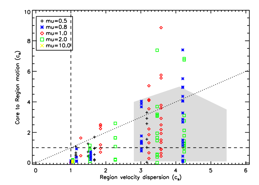
We analyze a suite of thin sheet magnetohydrodynamical simulations based on the formulation of Basu, Ciolek, Dapp & Wurster. These simulations allow us to examine the observational consequences to a star-forming region of varying the input level of turbulence (between thermal and a Mach number of 4) and the initial magnetic field strength corresponding to a range of mass to flux ratios between subcritical ($\mu_{0}=0.5$) and supercritical ($\mu_{0}=10$). The input turbulence is allowed to decay over the duration of the simulation. We compare the measured observable quantities with those found from surveying the Perseus molecular cloud. We find that only the most turbulent of simulations (high Mach number and weak magnetic field) have sufficient large-scale velocity dispersion (at $\sim$1 pc) to match that observed across extinction regions in Perseus. Generally, the simulated core ($\sim$0.02 pc) and line of sight velocity dispersions provide a decent match to observations. The motion between the simulated core and its local environment, however, is far too large in simulations with high large-scale velocity dispersion.

1 INTRODUCTION

The study of star formation is no longer in its infancy. Both observational and theoretical advances have taken the field beyond simple descriptions and heuristic models toward a more critical examination of the physical processes involved in assembling a star within a molecular cloud. Indeed, perhaps the biggest advance in star formation studies has been the ability to connect the formation of a star with the physical properties of the molecular cloud. Theorists and simulators have thus begun to model the larger scale properties of the molecular cloud to attack the stellar Initial Mass Function (IMF) and the star formation efficiency (SFE) (see review by Bonnell, Larson, & Zinnecker, 2007). At the same time, observers have begun to investigate statistically meaningful samples of prestellar cores and protostars, often within a single star-forming region (see reviews by Di Francesco et al., 2007; Ward-Thompson et al., 2007).

Most stars are born in groups and associations (Lada & Lada, 2003), thus the traditional pursuit of how an isolated star forms requires either an interest in a small subset of all stars or a hope that the underlying physics of star formation is not dominated by conditions external to the local prenatal core. These investigations have nevertheless proved to be extremely useful, yielding a simple yet powerful five stage model (prestellar/Class0-III) for the collapse and ignition of an isolated stellar-mass core (Lada, 1987; André, Ward-Thompson, & Barsony, 1993). In this manner, the timescale for collapse, the evolution of the accretion luminosity, and the formation of disks and jets has been examined both theoretically and observationally (Terebey et al., 1984; Henriksen et al., 1997; Shu et al., 1994). It is hoped that if the initial physical conditions in the core can be characterized - mass, temperature, turbulent energy, angular momentum, magnetic field strength and geometry - the stellar (plus disk) properties can be inferred (at least probabilistically).

Once the simplifying assumptions of isolated collapse are removed, physical intuition becomes more difficult. Theoretical calculations become complex, and simulations take precedence in attempting to discern how a molecular cloud fragments into stars. The large discrepancy between the Jeans mass in the cloud, typically tens to hundreds of Solar masses, and the mass of either the total cloud (typically hundreds of thousands of Solar masses) or the average star formed (typically around half a Solar mass) provides incentive for studies which take star formation to be part of the evolution of the cloud itself. In this scenario, there may never be an equilibrium core stage and the final distribution of stars may be determined by the flow of mass, energy, and magnetic fields within the evolving cloud. A large compendium of work on this topic is now available (e.g., MacLow & Klessen, 2004; Elmegreen, 2007).

Despite the complexity inherent in following the star formation process from the molecular cloud through dense core formation to the collapse to individual stars, the final outcome is quantifiable. Most simulations thus start with a particular set of initial conditions, evolve the cloud, and compare the outcome with observable quantities, primarily the IMF and SFE. The initial conditions usually attempt to recreate the observed physical conditions within the bulk cloud, concentrating on the additional support beyond thermal motion that keeps the bulk cloud from collapsing and fragmenting on a dynamical time. Thus supersonic turbulence and/or magnetic fields are utilized to provide partial support, at least initially, to the cloud. As the turbulence decays and the neutrals slip past the ions, gravity becomes dominant and the cloud collapses. Occasionally a suite of simulations with a range of initial conditions are computed and thus the variety in outcomes can be examined (e.g., Basu, Ciolek & Wurster, 2009; Basu, Ciolek, Dapp & Wurster, 2009, hereafter BCW09 and BCDW09 respectively).

Recent observations are providing new and more stringent conditions on the simulations. It is now possible to observe the dense gas and dust within an entire molecular cloud, revealing the manner in which structure forms - location, mass function, etc (e.g., Onishi et al. 1998; Johnstone, Di Francesco & Kirk 2004; Hatchell et al. 2005; Kirk, Johnstone & Di Francesco 2006, hereafter KJD06; Di Francesco et al. 2007; Ward-Thompson et al. 2007). As well, the kinematics of these dense cores and their surrounding envelopes can be detailed (e.g., Benson & Myers 1989; Jijina et al. 1999; Walsh et al. 2004, 2007; Kirk, Johnstone & Tafalla 2007, hereafter KJT07). It is thus time to consider how to utilize these additional constraints on star formation within the simulations.

In this paper we consider how to appropriately ‘observe’ a molecular cloud simulation in order to compare the model output with the properties of real star-forming clouds. In §2 we describe the details of the numerical simulations. In §3 we introduce the observational data set used in this analysis. §4 discusses the manner in which the simulations are ‘observed’ while §5 discusses the results and compares with the observations. Finally, we relate the results back to the larger theoretical framework in §6 and conclude in §7. In Appendix A we furthermore show that the trends found in the preceding sections are robust.

2 SIMULATIONS

2.1 General Overview of Simulations

In order to analyze the interplay between the competing processes responsible for converting molecular cloud material into stars, along with the ensuing physical attributes, it is necessary to run (magneto)hydrodynamic simulations (see review by MacLow & Klessen, 2004). The purpose of the present paper is to test which simulations show similarities with the observations of real molecular clouds and which observable measures provide the best discrimination between simulations with different initial conditions. We thus begin with a brief overview of the evolutionary implications of both turbulence and magnetic fields within molecular clouds, in order to set the stage for the results which follow.

In almost all simulations, the initial conditions begin with much more mass than can be supported under a simple thermal Jeans calculation. From the start of the calculation, the region is therefore inherently unstable to collapse unless additional processes are at play. Global gravitational collapse is typically delayed via the inclusion of initial supersonic turbulent motions. In keeping with both observations (e.g., Larson, 1981) and theoretical considerations, the largest length scales dominate the input turbulence. The simulated cloud therefore initially forms sheets and filaments with box crossing lengths, and it is within these over-dense regions that collapse takes place. Given the dynamic and fast evolution of these clouds, the applied initial conditions are extremely important and the explicit results should be taken with caution. The simulations provide instead an ideal laboratory for considering the time, length, and mass scales, and the efficiency of turbulent induced star formation.

An alternate mechanism which can significantly delay the global collapse of the simulated cloud is the inclusion of strong magnetic fields. The low density and moderate ionization fraction within molecular clouds leads to effective field freezing and thus magnetic fields act as an additional buoyant force opposing gravity. In sheet-like geometries, sufficiently strong magnetic fields are capable of overcoming gravity entirely and preventing collapse for an ambipolar diffusion time during which the neutral particles diffuse past the load-bearing, magnetic-field-coupled ions, eventually accumulating approximately a Jeans mass of material which is then capable of gravitational collapse.

While it is possible that either of these approaches alone may be responsible for delaying global cloud collapse, it is more likely that they are both present in which case the interplay between them is not at all straightforward. In addition to turbulence included in the initial conditions of a simulation, significant non-thermal motions can be generated through the gravitational collapse of non-uniformly distributed material (e.g., Burkert & Hartmann 2004). While magnetic fields oppose gravity by applying additional pressure support, supersonic turbulence both opposes gravity through enhanced kinetic energy in the gas and aids gravity through strongly compressive shocks. When both turbulence and magnetic fields are present, the turbulent shocks can be suppressed by magnetic fields. Even small enhancements in the density within these compressed regions, however, can significantly lower the ambipolar diffusion time. Meanwhile, shock compressions and rarefractions dissipate energy from the turbulent waves themselves, producing a competition between decaying turbulence and ambipolar diffusion.

Parameter studies following the evolution of molecular clouds with both magnetic fields and turbulence are greatly needed. The complicated numerical equations that must be solved in such cases make such simulations computationally expensive, however. Few large parameter studies have thus been carried out. Here, we utilize an extensive study (BCDW09) which followed the evolution of a sheet-like cloud in which significant simplifications are possible. The resolution of the simulations (128 by 128 cells) is modest, however, this is sufficient for our purposes – the simulations resolve the critical thermal length with a minimum of sixteen pixels and are stopped at an early enough stage that grid-scale fragmentation has not occurred. The analysis of BCDW09 further demonstrates the lack of impact that higher resolution has on the evolution of these simulations. As well, in Appendix B, we include our own analysis of higher resolution simulations (512 by 512 cells), which demonstrate that the coarser resolution simulations are adequate. We also note that while the geometry is simplified, and thus the turbulence and magnetic fields are idealized and unlike those expected in true three dimensional clouds, we are not attempting to prove any particular set of parameters as ‘true’. Our goal is less ambitious: to determine the effect of the input parameters on observables.

We note that there are other aspects of the input parameters that still remain to be properly investigated. In particular, whether turbulent energy does indeed decay or is driven (see the recent analysis of simulated dense core observables by Offner et al., 2008). Other simulations have addressed this issue in order to determine the scale on which driving would need to occur to prevent collapse of cores (e.g., Klessen et al., 2005). This remains, however, an open question to be considered with respect to the competition between magnetic fields and turbulence.

2.2 Details of the Simulations

Ciolek & Basu (2006, hereafter CB06) and BCW09 introduce and discuss in detail the setup and equations governing the evolution of the simulation with linear perturbations (see also Basu & Ciolek, 2004). The setup of simulations with turbulent intial conditions are discussed in BCDW09. Here, a few key details are highlighted. Note that the scalings applied to the simulation in order to convert from scale-free to observable quantities are given in Section 4.1. The simulations we analyze have a thin sheet geometry and are supported in the vertical direction by thermal pressure working against gravity and magnetic pinching. In the lateral direction, the evolution is governed by the interplay of thermal pressure, gravity, magnetic pinching and magnetic tension; see CB06 for a discussion on the physical justification and a detailed description of this geometry. The simulations start with uniform column density and a constant vertical magnetic field. Velocity perturbations are added in Fourier space to wavenumbers $k$ corresponding to wavelengths up to the simulation length in both the x and y direction. Velocity amplitudes are chosen from a Gaussian distribution scaled to the power spectrum $v_{k}^{2}\propto k^{-4}$ (i.e., most of the power is on the largest scales). The turbulent energy in these simulations is not driven but is allowed to decay. Unlike some purely turbulent simulations, gravity is always “on”; there is no initial period where turbulence is driven without gravity.

The material in the simulation is bounded in the direction perpendicular to the sheet by external pressure and gravity, as well as smaller contributions from magnetic pressure and magnetic tension. The relative importance of the former two quantities is expressed by the dimensionless parameter $\widetilde{P}_{\rm{ext}}$, the initial ratio of the external pressure to the self-gravitational pressure of the sheet in the vertical direction. We analyze simulations where the external pressure is minimal and the sheets are gravitationally dominated ($\widetilde{P}_{\rm{ext}}=0.1$), not unreasonable for the denser regions within molecular clouds. The other extreme, where the sheet is dominated by external pressure, would be appropriate in a situation where star formation is triggered by a supernova shock wave, for example. BCW09 analyzed a suite of simulations with both weak and strong external pressures ($\widetilde{P}_{\rm{ext}}=0.1$ and 10) and found that high external pressure environments lead to the formation of much smaller cores that attain high column density significantly faster than their low external pressure counterparts.

Considering only thermal support, the simulations begin with gravitationally unstable conditions. In the absence of external pressure, the simulations have a length of eight times the critical thermal length, or four times the lengthscale of maximum growth (see CB06 for further discussion), thus approximately sixteen objects would be expected to form. Additional support can be derived from both the input magnetic fields and turbulent velocity. We analyze simulations ranging from subcritical mass to magnetic flux ratios where there is no gravitational collapse possible without ambipolar diffusion ($\mu_{0}=0.5$ and 0.8), to critical ($\mu_{0}=1$), and supercritical ($\mu_{0}=2$ and 10). The turbulent velocity field input varies from having essentially no turbulent velocity (thermal Mach number of 0) to a Mach number of 4 in integer steps. Note that the simulations with higher Mach numbers, particularly Mach 4, showed significant qualitative differences from observations as discussed in Section 4.4, hence simulations with even higher Mach numbers were not run.

The simulations are evolved until a column density of ten times the initial uniform value is reached. Figure 1 shows two sample column density maps from the suite of simulations we analyzed. In simulations where the pressure from the magnetic field exceeds the pressure from the input turbulent motions, the magnetic field has a strong influence on the dynamics of the simulation. In particular, turbulent compressions are moderated by the restoring force of the magnetic field, hence density enhancements are smaller and tend to rebound rather than collapse due to gravity. When the magnetic fields are strong, the simulations thus require longer periods of time to reach a column density sufficient for the simulation to stop. The input turbulence is therefore able to decay to a much greater extent in these simulations than in turbulence-dominated ones. This causes the large-scale velocity dispersions to be smaller in the strongly magnetic simulations than their weakly magnetic counterparts, as seen in the analysis below. We postpone a full analysis of how the turbulent velocity field changes over the run of the simulation in these cases for a future paper.

3 OBSERVATIONS

3.1 Summary of Previous Results

Previously, we conducted a large-scale pointed survey of cores and their dynamics in the Perseus molecular cloud (Kirk, Johnstone & Tafalla, 2007). The Perseus molecular cloud is an intermediate mass star forming region located at a distance of $\sim$250 pc (e.g., ${\rm\breve{C}}$ernis, 1993) that displays more active and clustered star formation than seen in the low mass Taurus star forming region, but much less than seen in the high mass Orion star forming region. Our survey was thus ideal for probing the conditions of a more clustered mode of star formation without suffering from the complexity present in a region such as Orion. The dense core candidates were selected from cores observed in the submillimetre continuum using SCUBA (KJD06) and supplemented with visually-selected regions of higher extinction in the Palomar plates (and large-scale 2MASS extinction peaks). In our survey, we made single-point observations of dense core candidates simultaneously in N₂H⁺(1-0) and C¹⁸O(2-1), with beamsizes of 25″ and 11″ respectively, using the IRAM 30 m telescope in Spain. N₂H⁺ is a good tracer of dense gas, with a critical density of $\sim 10^{5}$ cm^-3 (Tafalla et al., 2002), while C¹⁸O traces lower density gas (critical density of $\sim 10^{3}$ cm^-3 Ungerechts et al., 1997) and freezes out of the gas phase onto dust grains at $\sim 10^{5}$ cm^-3 (Tafalla et al., 2002), hence the survey obtained information simultanenously about the dense core and the surrounding ‘envelope’ of material. We differentiated between protostars and starless cores on the basis of Spitzer data (Jørgensen et al., 2007). Supplemental information is also available from the COMPLETE Survey (Ridge et al., 2006) – large scale column density measures from stellar reddening observed with 2MASS (Alves & Lombardi in prep) using the NICER technique (Lombardi & Alves, 2001) as well as ¹²CO and ¹³CO FCRAO observations across the cloud (Ridge et al., 2006).

The survey of KJT07, based on submillimetre dust emission and optical / near-IR dust extinction - identified cores provides a useful set of dynamical constraints that simulations of star formation should match; we highlight several which are relevant to this work.

1) Cores have little internal turbulence. Starless cores have velocity dispersions which are dominated by thermal motions; protostars tend to have slightly larger (but still thermally-dominated) velocity dispersions. This result has been found by many other surveys including Benson & Myers (1989) and Jijina et al. (1999).

2) Material surrounding cores has a larger velocity dispersion. The less-dense material (traced by C¹⁸O in our survey) surrounding the dense cores tends to display much larger non-thermal motions, also consistent with previous observations (e.g., Benson & Myers, 1989; Jijina et al., 1999).

3) The relative velocity between the core and surrounding material is small. The vast majority of dense cores (nearly 90%) have less than thermal motions with respect to their surrounding material. Previous observations (Walsh et al., 2004, 2007) concur with this result.

3.2 Additional Observations

In order to compare our previous results with the analysis of simulation data below, we must fold in a few additional pieces of information about larger scales. First, we note that the dense cores in Perseus are clustered within larger-scale regions, as seen in the 2MASS extinction map. We defined these regions in KJD06 (referred to there as ‘extinction super cores’ and here as ‘extinction regions’ for clarity); here we adopt the size and mass estimates of these regions from KJD06 (typically 10′ and several hundred solar masses; see Table 1). These regions have roughly comparable sizes and masses to that found in the simulated box as discussed in the following section.

Additionally, we use the ¹³CO data from COMPLETE (Ridge et al., 2006) to gather information on the dynamics of each extinction region. While the spatial resolution of this data cube is lower (46″) than our IRAM C¹⁸O data, it has the advantage of uniformly covering each extinction region rather than sampling a set of sparse and biased locations. We calculate the velocity dispersion along each line of sight by fitting a single Gaussian to each ¹³CO spectrum. Additionally, we calculate the total velocity dispersion seen in each extinction region by summing all of the spectra within the extinction region and fitting the resultant spectrum with a single Gaussian. The ¹³CO data cube has a smaller areal coverage than the extinction map thus we only consider the eight of eleven extinction regions that have $>80\%$ coverage in the ¹³CO data cube. For each extinction region, Table 1 gives the region number, the mass, the radius, the velocity dispersion required to prevent gravitational collapse (in Gaussian sigma units), the observed velocity dispersion in ¹³CO (in Gaussian sigma units), the percentage of the region observed in ¹³CO, and a descriptive location. For those extinction regions which have at least 80% coverage in the ¹³CO data, Table 2 gives the observed ¹³CO velocity dispersion relative to the sound speed (assuming a temperature of 15 K), the number of dense cores identified in the SCUBA data of KJD06, the number of dense cores observed in the IRAM data of KJT07, and the estimated percentage of the region’s mass found in each set of dense cores (or core formation efficiency; the calculation of the number and mass of dense cores in each region is discussed in more detail in §5.4).

4 ‘OBSERVING’ THE SIMULATIONS

4.1 Scalings

The simulations are scale-free, with units in terms of the mean density and sound speed. To convert to observable quantities, we adopt the nominal pressure scaling of Ciolek & Basu (2006), a density scaling roughly three times their nominal density, plus the temperature and distance we previously adopted for our observations of the Perseus molecular cloud in KJD06 and KJT07, i.e., :

$$n_{n,0}=10^{4}~{}{\rm cm}^{-3}$$ (1)

$$T=15~{}{\rm K}$$ (2)

$$D=250~{}{\rm pc}$$ (3)

Recall that we analyze simulations where the sheet is gravitationally dominated with minimal external pressure, i.e,

$$\widetilde{P}_{\rm{ext}}=0.1$$ (4)

Using these scalings, the box length of the simulated region is 1.5 pc corresponding to an angular size of 21′ at the distance of the Perseus molecular cloud. This is comparable to the sizes of the largest structures identified in the extinction maps of KJD06 (see Table 1). Each pixel in the simulation is 0.012 pc, corresponding to an angular size of 9.8″, somewhat smaller than the beamsize of our SCUBA and IRAM observations. The mean initial column density is 3.5 $\times 10^{21}$ cm^-2, corresponding to a value of 1 in the scale-free simulations. If we adopt a dust opacity of $\kappa_{850}=0.02$ cm² g^-1 and a dust temperature of 15 K (and assume a dust-to-gas ratio of 1:100) for our SCUBA observations, then 1 Jy bm^-1 corresponds to $N_{H}=6.37\times 10^{22}$ cm^-2 and the mean column density in the simulation corresponds to 55 mJy bm^-1 .

The simulations are stopped when the maximum column density in the simulation reaches approximately a factor of 10 times the initial value, or $\sim 3.5\times 10^{22}$ cm^-2 (corresponding to a density of $\sim 10^{6}$ cm^-3). In simulations with strong turbulence and weak magnetic fields, this maximum is reached quickly, while in simulations with strong magnetic fields, more time is required to reach the maximum. The time each simulation runs is given in Table 3 in units of $t_{0}$ :

$$t_{0}\equiv\frac{c_{s}}{2\pi G\sigma_{n,0}}$$ (5)

where c_s is the sound speed, G the gravitational constant, and $\sigma_{n,0}$ the initial column density in the simulation (see CB06). The unit of $t_{0}$ is related to the sound crossing time of the sheet – when thermal pressure is the dominant term in determining the thickness of the sheet, we can write

$$t_{0}=\frac{Z_{0}}{2c_{s}}$$ (6)

(using eqn 13 of CB06), where Z₀ is the initial half-thickness of the sheet. Thus $t_{0}$ is approximately one quarter the sound crossing time of the entire thickness of the sheet. In their linear analysis, CB06 found that away from the critical mass to magnetic flux ratio ($\mu_{0}=1$), the lengthscale for maximum growth of instabilities was 2$\lambda_{T}$ where $\lambda_{T}$ is the critical thermal length scale given by

$$\lambda_{T}=\pi\Big{(}\frac{1+3\widetilde{P}_{\rm{ext}}}{1+\widetilde{P}_{\rm{ext}}}\Big{)}Z_{0}$$ (7)

(CB06 eqn 40), or $\lambda_{T}\simeq\pi Z_{0}$ for a low external pressure environment. Thus the sound crossing time across the lengthscale of maximum growth is $4\pi t_{0}$. Table 3 shows that in the non-turbulent simulations, the run-time for the weakest magnetic field cases is roughly equal to this timescale. In the highly turbulent simulations, the run-time can reach a few tenths of $t_{0}$, much shorter than even the turbulent crossing timescale of the linear lengthscale of maximum growth. This implies that in these highly turbulent simulations, the resultant peaks are due to compressions directly from the input initial conditions, as there has not been sufficient time for gravitational information to have propagated across the relevant lengthscales. Note that the entire length of the simulated box is 16$\pi c_{s}t_{0}$ or 8 $\pi Z_{0}$, corresponding to four times the lengthscale of maximal growth for a low pressure environment with a mass to magnetic flux ratio away from critical. All of the turbulent simulations are therefore stopped well before the thermal crossing time of the box, $16\pi t_{0}$.

Figure 2 shows several examples of well-known star forming regions in Perseus observed in the submillimetre while Figure 3 shows the same example simulations as shown in Figure 1 but scaled to the same flux range and size as the observations. White noise has been added to the simulations at approximately the same level as is present in the observations.

4.2 Identification of Simulated Cores

Direct comparison can be made between the column density structure found in the simulations and observations, since both are two-dimensional projections. This is not, however, the case for comparing dynamics. Since the velocity is only calculated in the two dimensions of the simulation, the simulations must be considered in a one dimensional projection along x or y in order to obtain the motion towards or away from an observer. We first project the column density map in the x and y directions to identify density peaks. Since the simulated sheet is thin, we do not account for changes in the projected column density due to variations in the thickness of the sheet. Note that the locations of peaks in the one dimensional projections tend to have good correspondence with overdensities in the original two dimensional column density map, although there can be differences where two structures lie along the same line of sight (particularly for filamentary structures seen in the highly turbulent simulations). Figure 4 shows examples of the projected 1D column density.

To identify cores, we find all the peaks in the projected column density which lie above a specified threshold and are separated by at least one IRAM N₂H⁺ beam. We set the minimum peak threshold to a value corresponding to the typical column density threshold we would expect in two dimensions – assuming a typical core spans little more than an IRAM N₂H⁺ beam (3 pixels), and has a minimum column density threshold of 3 times the mean (which, for particles uniformly distributed along the column corresponds to a density of 9 $\times 10^{4}$ cm^-3, roughly the critical density of N₂H⁺), then the minimum 1D column density is $(N-3)\times 1\sigma_{0}+3\times 3\sigma_{0}$, where $\sigma_{0}$ is the mean column density (1) and $N$ is the number of pixels in the simulation in 1D (128). This core identification is designed to mimic our observational method as best as is possible (N₂H⁺ targets in KJT07 were based on dust column density measurements, primarily from SCUBA data). Note that the results in our later analysis show little variation with any changes in the peak identification parameters (see Appendix A for further details).

4.3 Calculation of Simulated Spectra

As described in §2, our IRAM survey consisted of pointed observations of dense cores in two molecules – N₂H⁺, which traces the dense gas, and C¹⁸O which only traces the less dense gas. For every peak identified in the simulations, we can calculate spectra corresponding to both of these tracers. For each projected 1D peak, we consider the material along the corresponding line of sight and split it into the dense material (cells with values above 3 times the mean column density), corresponding to the material which N₂H⁺ traces, and less dense material (cells with values less than 3 times the mean column density), corresponding to the material which C¹⁸O traces. This threshold corresponds to a mean density of $9\times 10^{4}$ cm^-3 or nearly $10^{5}$ cm^-3. We then calculate the spectra by assuming that each cell emits a thermally broadened Gaussian centred on the velocity of that cell and weighted by the amount of material (column density) present in that cell. For clarity, we term the two spectra calculated for every 1D column density peak as the core (high density gas) spectrum, which corresponds to the N₂H⁺ dense core spectrum, and the LOS LDG (line of sight low density gas) spectrum, which corresponds to the C¹⁸O ‘envelope’ spectrum. Figure 5 shows two example sets of core and LOS LDG spectra.

As an aside, we note that the LOS LDG spectra are little affected by the exclusion of material above a column density threshold, rather than all material along the line of sight. The physical basis for this is that the majority of the mass is found in the lower density material, so the behaviour of the high density material has very little effect on a cumulative spectrum. This is demonstrated in Figure 6 which shows spectra of the core (top panel), the LOS LDG material used in our regular calculations (middle panel), and all material along the LOS (bottom panel). This is one of many cases we found where the simulated core spectral peak lies roughly in the minimum between two spectral peaks in the associated LOS LDG material. Clearly, the addition of the extra material in determining the LOS spectrum (bottom panel) has very little effect on the LOS LDG spectrum. This is important, as it demonstrates that our choice of column density threshold for the LOS LDG material has little effect on the measure of core to LOS LDG velocity difference (see also Appendix A).

In our IRAM survey, the beamsize of the N₂H⁺ observations is more than twice as large as the C¹⁸O observations (25″ and 11″ respectively), as mentioned in §3. In our calculation of the simulation ‘observables’, we similarly consider cells within the appropriate beamsize (3 pixels for the core, 1 pixel for the LOS LDG) for their contribution to each spectrum. An odd number of pixels is necessary to allow an equal sampling on either side of the core’s peak.

A few peaks identified in the 1D projection have no cells within the beam above the (column) density threshold set for the core material. This occurs where two lower density structures, e.g. filaments, lie along the same line of sight, usually in the high turbulence simulations where the structure is less regular. We use data from these points only in our analysis of the distribution of LOS LDG velocity dispersions. This is analagous to our IRAM data, for which we had a few more detections in C¹⁸O than in N₂H⁺ of candidate dense cores.

We also create spectra to compare with the ¹³CO FCRAO observations. Like C¹⁸O, the ¹³CO observations trace the lower density material, however, we have ¹³CO observations across the entire Perseus cloud (albeit at a lower resolution than our C¹⁸O observations). These observations allow us to gain a more global understanding of the dynamics of lower density material on larger scales. We therefore calculate LDG spectra along every LOS of the simulations using a beamsize of 5 pixels to correspond to the 46″ beam of the ¹³CO data (i.e., 26 = 128/5 spectra for each x and y projection of a simulation). These simulated spectra can be thought of as arising from a chord across the projected centre of the star-forming region, and thus we compare these spectra with ¹³CO spectra that run across the approximate centre (in right ascension and declination) of each extinction region. Comparison with all observed ¹³CO spectra in the extinction region instead of only the central chord would include a larger fraction of lines of sight that pierce only the small edge of the 3D cloud, whereas the simulations trace the mid-plane of the cloud only.

4.4 ‘Observed’ Properties

We fit the resultant core and associated LOS LDG spectra with Gaussians – a single Gaussian where possible, and two Gaussians where the fit is significantly improved; this method was also used in our IRAM survey. Figure 5 shows some examples of the spectra generated.

Simulations with strong turbulence tend to produce spectra which are more irregular and not well-fit even with a double Gaussian. In KJT07, we found that N₂H⁺ dense core spectra were well fit by single (and occasionally double) Gaussians, and the C¹⁸O spectra were mostly well fit by single or double Gaussians. The poorer fits in the simulated spectra for the high input turbulence suggests that these simulations are qualitatively different than the observed regions.

We used our Gaussian fits of the simulated spectra to identify the relevant dynamical properties of each core and associated LOS LDG material – linewidth and centroid velocity. In the following sections, we analyze these results and compare them with the observational analyses in KJT07. Note that while a small number of cores are identified in a given simulation, small number statistics are not a major concern, i.e., similar properties are measured across multiple simulations run with the same input Mach number and magnetic field strength.

For the larger-scale LDG LOS simulated spectra corresponding to our ¹³CO observations, we found that both the simulated and observed spectra were less well described by a Gaussian fit. Since our analysis of these spectra requires only a measurement of the linewidth, we found that measuring the full width of the emission at one quarter of the peak (FWQM) was effective. Figure 7 shows an example of a simulated larger-scale LOS LDG spectrum in one of the most turbulent simulations. As seen in the figure, we found the width of the emission at half of the peak (FWHM) often picked out narrow emission peaks while missing underlying wide emission, while the FWQM was sensitive to the wider emission underneath. Measurement at levels lower than the quarter maximum sometimes presented a problem for the ¹³CO observations where these levels became too close to the noise level. Where multiple peaks were found to be separated even at the quarter maximum, we only counted regions above the quarter max for our width measurement. This was especially important in our ¹³CO observations to prevent bias from large noise spikes. (Note we also smoothed our ¹³CO spectra to five spectral channels, or 0.33 km s^-1 to reduce errors introduced by noise.) For a single Gaussian, the FWQM can be converted to a Gaussian $\sigma$ through division by $4\sqrt{\ln{2}}$ or $\sim 3.3$. We refer to the Gaussian $\sigma$ corresponding to the measured FWQM as the “effective” velocity dispersion.

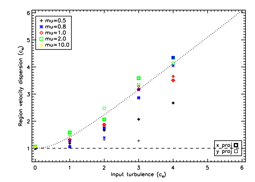
Finally, we created a composite spectrum describing the whole of each simulation (in both projections), and similarly summed all of the ¹³CO spectra within each extinction region. To estimate the velocity dispersion of the entire region, we fit these spectra with a single Gaussian, which provides reasonable agreement. Note that in the simulations with weak magnetic fields, the velocity dispersion measured is nearly identical to what would be expected from the input turbulence level; simulations with stronger magnetic fields tend to have lower measured dispersions due to damping of the turbulence. Figure 8 shows the velocity dispersion found across the simulation as a whole versus the level of input turbulence. In our observations, we only include 8 of the 11 extinction regions identified in KJD06, as the other 3 have poor coverage ($<80\%$) in the ¹³CO map which prevents proper measurement of the dynamics.

Table 4 provides the overall statistics for all of the ‘observed’ dynamic quantities in the simulation – the mean and standard deviation of the velocity dispersion of the LDG material along all lines of sight (corresponding to the ¹³CO observations), the velocity dispersion of the LDG material along lines of sight where dense cores were identified (corresponding to the C¹⁸O observations), the velocity dispersion of the dense cores (corresponding to the N₂H⁺ observations), and the difference in centroid velocity between the core and LOS LDG material. Table 5 shows the number of cores found in each simulation and the percentage of mass found within the cores (core formation efficiency, or CFE). Note that Appendix B includes the analysis of several higher resolution simulations and demonstrates that the resolution does not affect the ‘observable’ dynamic quantities reported here.

5 RESULTS

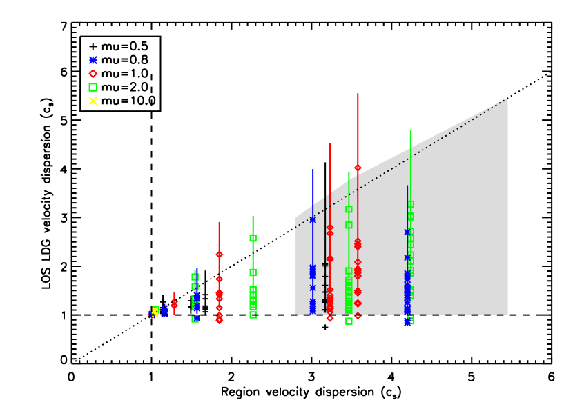
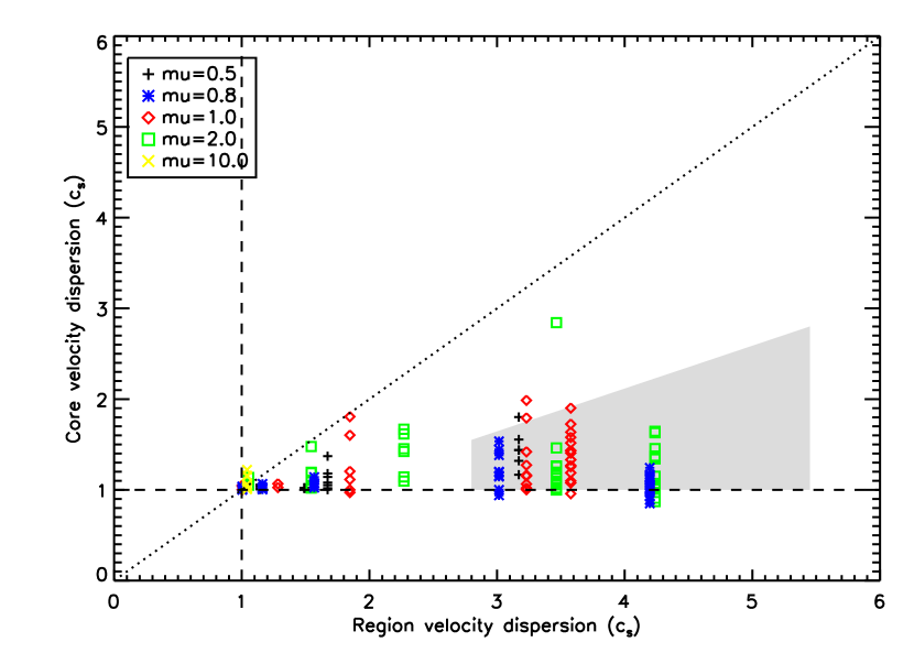
5.1 Internal Velocity Dispersion

5.1.1 Across the Cloud

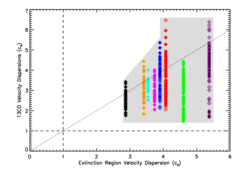
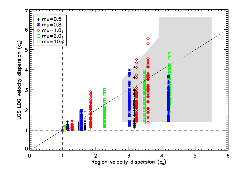
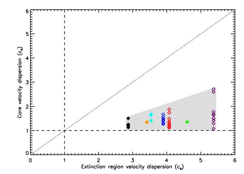
We first examine the behaviour of the larger-scale, less dense material in order to gain perspective on the environments in which the dense cores form. In Figure 9, we show the effective velocity dispersions observed in ¹³CO along two central chords (in right ascension and declination) through each extinction region versus the velocity dispersion observed for the entire extinction region. (Note that the observational results do not change significantly if all lines of sight in the extinction region are used instead.) In Figure 10, we show the corresponding measurements for the simulations – the effective velocity dispersions of LDG along all LOSs compared to the velocity dispersion of the simulated region as a whole. (These values are included in Table 4.) Both Figures 9 and 10 show a range in LDG velocity dispersions along individual LOSs, ranging from small to larger than the mean for the cloud as a whole. Note that while the range in individual LOS LDG velocity dispersions are similar for both the observations and simulations, the extinction regions observed in Perseus tend to have higher velocity dispersions as a whole than within the simulations. Only simulations with the highest input turbulence (Mach number 3 or 4) show regional velocity dispersions similar to the lower end of the range spanned by our ¹³CO observations. Since feedback is not included in the simulations, it may be more appropriate to compare the simulations only with regions in Perseus that do not appear to have formed previous generations of stars; the filled symbols in Figure 9 indicate the extinction regions which appear to have had less recent active star formation (i.e. excluding NGC1333, IC348, and B1). These regions do tend to have slightly lower regional velocity dispersions than their active star-forming counterparts.

5.1.2 LDG Along LOSs Associated with Dense Cores

We next examine the velocity dispersions seen in the LOS LDG material associated with the dense cores. As discussed above, the LOS LDG motion could provide hints for the scale of turbulence in the molecular cloud. There also may be a difference between lines of sight that contain cores and those that do not, if, for example, cores form at stagnation points in the velocity field. Our pointed IRAM C¹⁸O observations are at higher spatial resolution than the ¹³CO map, but still allow LOSs with cores to be compared with the overall distribution of LOS LDG dispersions.

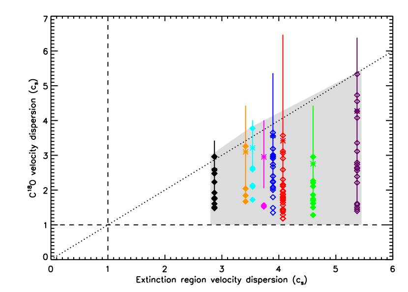
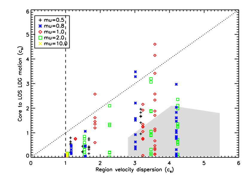
Figures 11 and 12 show the distribution of velocity dispersions measured for LOS LDG material where cores were detected (points) for the observations and simulations (at the higher resolution of the IRAM survey) versus the velocity dispersion of the entire region. Each figure also shows the distribution of LDG velocity dispersions (mean plus and minus the standard deviation) for all line of sight material (at lower resolution / larger beamsize). Note that as in the previous section, the larger-scale LOS LDG linewidths are measured from the FWQM, with only the LOSs along the central right ascension and declination line of the extinction regions included in the observed plot. The dashed lines show the minimum expected observationally, i.e., the thermal width, while the dotted line shows a 1:1 relationship between the velocity dispersion of the larger environment (simulated region or extinction region) and the LOS LDG material. The figures illustrate that the bulk of the LOS LDG material has a similar velocity dispersion to the larger environment, while the LDG along LOSs that contain cores often have much lower velocity dispersions. Note the spectral line-fitting technique and resolution could play a role in this difference – the FWQM measure used for the bulk of the LOS LDG spectra is more sensitive to low levels of extended velocity dispersion than a single (or double) component Gaussian fit which may preferentially probe the local core environment.

5.1.3 Dense Cores

We next turn our attention to the cores. Recall that emission from the dense cores originates from relatively compact regions of overdensity. In some turbulent simulations, dense cores are transient features of overdensity formed by the intersection of two colliding streams of material (Ballesteros-Paredes et al., 2003). In such a case, one might expect to see a large internal velocity dispersion within the core for some fraction of the population – although the centre of the turbulent compression typically has low velocity dispersion, the core as a whole can encompass a sufficiently large region so as to reveal a larger velocity dispersion. Indeed, in turbulent simulations for which the distribution of dense core internal velocity dispersions were calculated (Klessen et al., 2005; Ayliffe et al., 2007; Offner et al., 2008), a small but non-zero population of cores with supersonic internal velocity dispersions is present. In each case, the highest internal velocity dispersions in the simulations were larger than those seen in the observations of KJT07. On the other hand, cores which are bound and evolving more quiescently would be expected to have small internal velocity dispersions. As discussed in §3, previous dense core surveys (e.g., Benson & Myers, 1989; Jijina et al., 1999) found that dense cores have small, thermally dominated internal velocity dispersions, although some turbulent motion may still be present, as discussed in §3.

Figures 13 and 14 show the internal velocity dispersion of the cores with respect to their larger environment (the extinction / simulation region) versus the velocity dispersion of the entire region. The cores have a similar range of velocity dispersions in both the simulations and observations, although as noted previously, the observed cores tend to inhabit large-scale environments with higher turbulent energy.

5.2 Core-to-LOS Motions

A second discriminant between the various simulations as well as the observations is the relative motion of the core and the surrounding LOS LDG material. Observations indicate that cores do not have significant motions within their local environment, with most displaying smaller motions than either the mean velocity dispersion of their local environment or the local sound speed (Walsh et al. 2004, 2007; KJT07). Walsh et al. (2004) have argued that in the turbulent framework of star formation, if cores form via competitive accretion, one might expect to see significant motion between the core and its local environment. Some simulators have since argued that competitive accretion simulations can display similarly small velocity dispersions (Ayliffe et al., 2007). It is unclear, however, whether these simulations are able to simultaneously meet all observational constraints (e.g., both the core to envelope motions and core internal velocity dispersion; see KJT07, ). In any event, the motion between the core and its surrounding material is a useful measure to examine in the context of turbulent models.

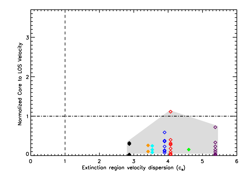
Figures 15 and 16 show the relative motions of cores and their LOS LDG material versus the velocity dispersion of the entire region for the Perseus observations and the simulations respectively. What is striking about the two figures is that observations display a much greater connection between the core and LOS LDG material – the differences in velocity are quite small despite having more non-thermal motion on larger scales. In the simulations, the core-to-LOS LDG motion becomes large even for only moderate large-scale velocity dispersions.

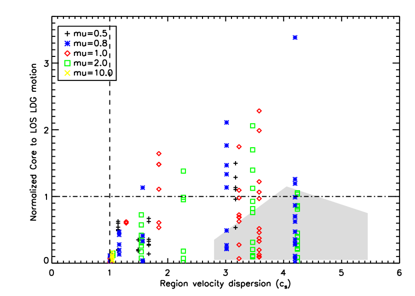
A second way to measure the motion is to compare the core-to-LOS LDG motion to the typical motion found in the LOS LDG material, i.e., the LOS LDG internal velocity dispersion. The difference between the observations and simulations using this measure are even more pronounced. Observations show the cores are quite quiescent within their nearby surroundings, while the simulations show cores often have motions larger than the LOS LDG velocity dispersion. Figures 17 and 18 show the core-to-LOS LDG motion divided by the LOS LDG velocity dispersion versus the velocity dispersion of the region as a whole.

In the simulations with high input Mach numbers, the LOS LDG spectra often had complex structures and most required fits with two Gaussians. In instances of two Gaussian fits, we selected the velocity component with the closest centroid velocity to compare with the core centroid velocity. This was also the procedure used in our IRAM observations in KJT07, although in that work we found fewer spectra that required multiple Gaussian fits than in the turbulent simulations, where LOS LDG material spectra frequently displayed more than two peaks. We visually checked all core and LOS LDG spectra and fits to ensure the Gaussian fits to the more complex structure did not bias the fits to higher velocity differences. We found there are a few cores where somewhat smaller velocity differences would have been obtained had all of the peaks in complex LOS LDG spectrum been used for the spectral fitting, however, there were also several instances where the velocity differences would have been larger had all the peaks been used in the spectral fitting. We therefore conclude that the overall effect on the velocity difference from using only two Gaussian components is negligible. Note that for the observations, the selection of the closest C¹⁸O velocity component did not bias the results to smaller velocity differences (see KJT07 for more details).

5.3 Core to Region Motions

In order to further investigate the large motions between core and associated LOS LDG material in the most turbulent simulations, we examined the motion between the core and the entire region. This provides an indication of whether the cores sit relatively unperturbed within the larger environment while the low density LOS material moves at high velocities, or whether both core and LOS LDG material move at (differing) high velocities.

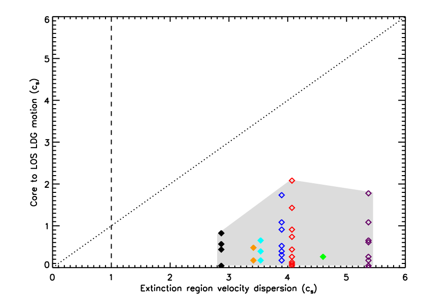
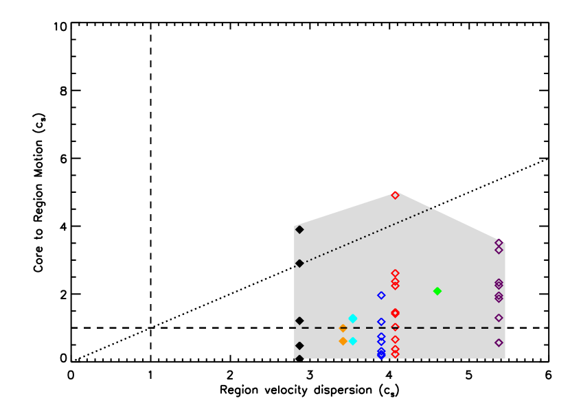
Figure 19 shows the absolute difference in centroid velocity between the observed dense cores and the extinction region as a whole versus the velocity dispersion of the extinction region. While a significant fraction of the cores do display supersonic motions, nearly all have motions that are significantly smaller than the total velocity dispersion observed in the region. The velocity dispersion of each extinction region tends to be similar (within a factor of 1.5) to that required for the region to be in energy equipartition between gravitational and internal kinetic energy (Table 1) . This implies that the dense cores observed tend to move with sub-virial velocities.

Such small velocities are not seen in the simulations, however. Figure 20 shows the absolute difference in centroid velocities between the dense core and the region as a whole versus the velocity dispersion of the region. This indicates that the dense cores can reach quite large velocities with respect to the simulated region as a whole (the centroid velocity of the region is nearly zero as one would expect). Figure 20 shows that the simulated cores often move much faster than the sound speed, and sometimes even in excess of twice that of the velocity dispersion of the region as a whole! In these simulations, the timescale for the formation of the first high column density peak is very short – much less than a crossing time (see Table 3). The short timeframe before dense structure formation allows some of the cores to inherit the kinematics of material at the high end of the velocity tail of the input turbulence. (Note that for every high velocity core, there are several at lower velocties in the same simulation.) The short simulation timescale also originates from the high velocity tail – high velocities lead to strong turbulent compressions which quickly compresses the column density to ten times the mean, at which point the simulation is stopped.

The observations therefore paint a picture of cores moving slowly with respect to their turbulent surroundings, whilst in the simulations, compressed density enhancements can be formed with a much greater velocities than their surroundings.

5.4 Formation Efficiency

The final quantities that can be compared between the simulations and the observations are the number and total mass of the cores formed within each region. Star formation is known to be an inefficient process, with the fraction of mass ending up in stars ranging from a few percent to a few tens of percent in clustered environments (Lada & Lada, 2003). Within the size scale probed by the simulation, the fraction of mass in dense cores is expected to be on the order of 10%, since this is a more clustered environment than the cloud as a whole. Jørgensen et al. (2008) found that protostars make up 17% of the mass within the clustered regions of Perseus and 3% of the mass of the cloud as a whole. Similarly, KJD06 found that dense cores make up roughly 1% of the entire cloud mass in Perseus.

Our observations, unfortunately, do not lend themselves to a straightforward computation of either the number of dense cores or the mass within them. Our IRAM N₂H⁺ survey, which is the basis for the calculations of dense core properties, was based on a target list created using several methods. The majority of targets were based on cores found in the SCUBA dust continuum map of the cloud, while a still significant fraction was based on visual selection of targets from Palomar plates. The SCUBA observations spanned roughly the entire Perseus molecular cloud (to A${}_{V}\sim 5$) so the list of N₂H⁺ dense cores that have an associated SCUBA source should be complete and unbiased. The Palomar plate targets, however, were explicitly drawn from areas with no SCUBA detections. We anticipate that our total list of dense cores detectable in N₂H⁺ is mostly (but not fully) complete, and may have slight biases in certain regions. We therefore provide two estimates of the number of cores observed per extinction region – the first being the number of N₂H⁺ cores associated with a SCUBA source, and the second being the total number of N₂H⁺ cores in our IRAM survey. The latter should provide a closer estimate of the total number, but different regions may have different fractions of cores missed. Table 2 provides both of these numbers for the eight extinction regions analyzed. The table shows that the number of cores varies between a few to nearly thirty, with only a small difference between the two estimates. Regions where star formation appears to have initiated more recently have less than ten cores per region.

The observed total mass of the cores within each extinction region provides a further challenge in calculation, and provides a second motivation for separating dense cores associated with SCUBA sources from the total population. The mass of the dense cores cannot be determined from our N₂H⁺ observations. The SCUBA observations, however, allow the mass to be determined (making assumptions about the dust opacity, temperature, etc) but the Palomar cores do not. We use our estimates of SCUBA masses from our 3″ map analysis (included in Table 6 of KJT07) and assume that the N₂H⁺ cores without an associated SCUBA source each have the median mass of the SCUBA sources (0.8 M_⊙). Since these N₂H⁺ cores were not detected with SCUBA, one might argue they are likely to have smaller masses than those with associated SCUBA sources, thus the reader is urged to treat the total core mass estimates for every extinction region as approximate. The fraction of mass in dense cores within every extinction region is calculated using the mass of the extinction regions found in KJD06. Table 2 shows the fraction of mass (core formation efficiency) found using both the N₂H⁺ SCUBA cores only and all N₂H⁺ cores. The fraction of mass in the dense cores tends to be on the order of a few percent using either measure, somewhat lower than in Lada & Lada (2003), however, that measure includes already-formed stars.

In the simulations, both the number of dense cores and the fraction of mass contained within the dense cores (core formation efficiency) are straightforward to calculate. Table 5 shows these values for the various simulations. As can be seen from the table, the simulations tend to form a small number of cores ($<$10), with the fraction of mass contained within them being of order a few percent. Since the simulations are stopped at a relatively early time-step (when a column density of ten times the mean has been reached), it is possible that further accretion and / or fragmentation could significantly alter these results.

6 DISCUSSION – INTERACTION OF THE MAGNETIC FIELD AND TURBULENCE

We take a step back from the simulations here to discuss some general trends and behaviors which arise from the combination of input turbulence and magnetic field.

The purely isothermal simulation ($M=0,\mu_{0}=10)$ reveals the scales expected from gravitational instability (eqn 7), since the only other physical parameter, the external pressure, provides merely a small perturbation. The simulation thus produces mostly round, dense cores each with approximately a critcal mass, forming out of a regular velocity field and undergoing gravitational collapse after about a sound crossing time of the critical length, or $\sim 12t_{0}$.

When turbulence is added to the isothermal scenario, there is the addition of a non-regular velocity field, with the largest kinematic modes found on the largest spatial scales. These supersonic velocity fields lead to shocks which create significant density enhancements – the ram pressure is $\sim\rho_{0}~{}M^{2}~{}c_{s}^{2}$, which produces compressions of $\sim M^{2}$ in the post-shocked, isothermal gas. The strongest density enhancements originate from the largest turbulent modes, forming long filaments in less than a turbulent crossing time across the region. For highly turbulent simulations, the initial conditions of the highly supersonic velocity field can produce column density enhancements strong enough to stop the simulations extremely quickly. The dense objects formed in these simulations tend to be more elongated than in the isothermal case due to non-uniform compressions, and the sizes of the cores formed are smaller since the Jeans length decreases with the higher density.

When magnetic fields are added without turbulence, the relevant size scale for collapse varies significantly as a function of the initial mass to flux ratio $\mu_{0}$ (CB06). The formed objects are mildly elongated (see BCW09, for a detailed discussion of the shapes), with a smooth velocity field. Strong magnetic fields, however, delay the formation of dense structures and gravitational collapse for an ambipolar-diffusion time, during which the neutrals slip past the load-bearing ions. For the conditions assumed here, the time to runaway collapse of the first core is about a factor of ten longer than in the isothermal nonmagnetic case.

When magnetic fields and turbulence are both present, the situation becomes much more complicated. For strong magnetic fields the magnetic pressure is sufficient to effectively prevent strong compressions even in turbulent velocity fields and evolution occurs only slowly via ambipolar diffusion. (Note that since we are analyzing thin sheet models with the magnetic field initially perpendicular to the sheet, compressions cannot act along the direction of the magnetic field lines.) In these cases, the final outcome will be similar to the case where only the magnetic field was present. For somewhat weaker magnetic fields, the turbulence is able to create significant compressions but the ram pressure is balanced by a post-shock enhanced magnetic field pressure in which the density increases by only $\sim M$ (Stahler & Palla, 2004) rather than by a post-shock thermal pressure at an enhanced density. In these compressed zones, the magnetic field enhancement effectively overwhelms gravity and collapse cannot occur until ambipolar diffusion removes the magnetic support. Given the higher density and shorter length scales involved, the ambipolar diffusion is nevertheless significantly shortened. Finally, when the magnetic fields are insignificant, even in the turbulently compressed regions, the simulation proceeds as in the purely turbulent case. Back of the envelope calculations show that the simulations we analyze fall in the regime of turbulent compression leading to significant magnetic field pressure; none have sufficiently weak fields to fall into the purely turbulent regime.

Will our results and conclusions differ dramatically if we consider three-dimensional simulations within the same physical parameter space? This is not likely, as demonstrated by the recent results of Kudoh & Basu (2008), who performed three-dimensional simulations of strongly and moderately magnetized clouds with initial turbulent fluctuations, including the effect of ambipolar diffusion. Their results are in general agreement with the thin-sheet calculations of Li & Nakamura (2004) and BCDW09. A large parameter study in three-dimensions, however, remains prohibitively expensive computationally. The special feature of our current work is that we are able to sample a large range of parameter space. Nevertheless, we do anticipate performing a similar study with three-dimensional simulations in the future, as broad parameter surveys become available.

Despite the above point, we note that different conclusions may yet be possible if we consider the case of continually driven turbulence or global (non-periodic) cloud models, in either the thin-sheet or three-dimensional cases.

7 CONCLUSIONS

Although the simulations we analyze have a thin sheet geometry, their relative simplicity provide the advantage of taking a relatively short amount of time to run, and hence easily allow a parameter study. While we do not expect the quantities measured here to be identical with a more complex, three-dimensional study, we do expect the trends we observe to be generally valid in the three-dimensional case as well.

From our analysis of the simulations we find the following:

• The large-scale (regional) low density gas velocity dispersions in the simulations tend to be lower than found in our observations. Simulations with strong magnetic fields tend to cause input turbulence to significantly damp by the time the simulation is halted for analysis (column overdensity of $\sim 10$).

• The velocity dispersions of the simulated dense cores tend to be low, in agreement with observations. The low density material along the same line of sight (LOS) tends to have larger velocity dispersion, as is also observed.

• The motion of the simulated core within its local environment (difference in core and LOS low density material centroid velocities) is large in simulations with high turbulence. This contradicts our observations that show cores have little motion with respect to their local environment, even in the clustered environment of Perseus.

It therefore appears that reconciling turbulence on large scales and quiescence on small scales (both within the core and between the core and envelope material) requires additional forces to soften the small-scale dynamics while allowing turbulent motions to remain on the large scales. Magnetic fields are a promising avenue to provide the small-scale damping of motions, however, in the simulations we analyzed, the large-scale turbulent motions also decayed, hence a mechanism would be required to renew large-scale turbulence. In the simulations we analyzed, the input turbulence is neither long-lived nor refreshed through the global evolution of the cloud or the formation of the first protostars, etc. The inclusion of further turbulent input after the start of the simulation thus might allow for supersonic motions to be observed on the large scale while preserving small scale quiescence.

The nature of the simulations themselves are also important to keep in mind – the simulations are done in the thin-sheet approximation and have periodic boundaries in the horizontal directions. This has some limitations, for example, magnetic field lines and turbulent vorticity can become tangled in three-dimensions in a manner that they cannot in thin-sheet models. The periodic boundaries can influence the coupling of turbulence on different scales, and also impose a rather arbitrary largest scale of turbulence in the simulation. We believe that the problem of maintaining very turbulent motions on large scales, while keeping cores relatively quiescent, may not be addressible in any periodic box model, whether thin-sheet or three dimensional, and may require a global approach to cloud modelling.

This study illustrates the power of utilizing kinematic ‘observables’ in simulations to discriminate between simulations with different initial conditions and to compare with observations, rather than limiting the analysis to quantities such as the mass function and star formation efficiency. This is an era where large (degree) -scale surveys are becoming more feasible (the COMPLETE Survey data used in part here will be eclipsed by more than an order of magnitude by the next generation of surveys, including the JCMT Gould’s Belt Legacy Surey (Ward-Thompson et al., 2007b) and the Herschel Gould’s Belt Legacy Survey (André & Saraceno, 2005)). Soon observers will be able to provide information on a statistically significant set of dense cores and their environment over the extent of many molecular clouds, which will provide much-needed information to constrain simulations of star formation. Simulators should start to prepare to take advantage of this vast increase in information when it arrives.

8 ACKNOWLEDGEMENTS

We thank the anonymous referee for the thorough review which improved our paper. HK would also like to acknowledge valuable discussions with people at the CfA, in particular Alyssa Goodman, Charles Lada, and Phil Myers, and Wolf Dapp (UWO) for a careful reading of our manuscript.

For the duration of this research, HK was supported by a Natural Sciences and Engineering Research Council of Canada (NSERC) CGS Award and a National Research Council of Canada (NRC) GSSSP Award. DJ and SB are supported by NSERC Discovery grants.

Appendix A EFFECT OF SCALINGS

The simulations we analyze are scale-free, which leads to the reasonable question of how dependent the results we find above are on the values of the scale factors (temperature, external pressure and mean density) we adopted in order to compare the simulations to observations. In this section, we address this question and demonstrate that a change in the scale factors has a minimal impact on the ‘observables’ derived and hence the results of our analysis. We start with a discussion of our motivation in choosing the values of the scale factors used in the above analysis, which gives a sense of the range that could have been applied. Next we show how modifications to the scale factor would effect our results.

A.1 Physical Motivation For Scalings

Converting the simulations into observable units requires one to assume a temperature, external pressure, and mean density. (Comparison to our observations requires a further assumption of the distance to the Perseus molecular cloud to convert the size observed from angular to physical.)

The temperature is constrained to a fairly small range by observations of star-forming regions, and hence does not tend to play a significant role in comparisons. Our previous observational results assumed that the temperature is 15 K everywhere. Recent ammonia observations have shown that dense cores in Perseus have a mean temperature of $\sim$12 K with a spread of only a few Kelvin (Rosolowsky et al., 2008); as discussed in KJT07, assuming a temperature of 15 K rather than 12 K does not have a large effect on our observational results. For ease of comparison with our previous work, we assume this temperature for the simulations as well.

The mean density, on the other hand, can be considered over a wider range of values, since star formation regions have a hierarchical structure in size and density. The dense cores we observed in our IRAM N₂H⁺ survey require densities of greater than or equal to $\sim 10^{5}$ cm^-3, in order to be observable. Thus the simulation must reach similar peak densities in order to be ‘observable’. Since the simulations are stopped when the maximum column density is ten times the mean column density, the corresponding mean (three-dimensional) density cannot be too low for N₂H⁺ to be detectable. The mean density also cannot be too large, as this would lead to a large fraction of the material in the simulation being at relatively high densities, while observations show that this is not the case (§5.4). Also note that a higher assumed mean density implies a smaller size for the region simulated (eqn 26 of CB06).

While the above physical arguments place some boundaries on the adopted scaling parameters, it is clear that there is an allowable range. A different choice in the adopted scaling parameters would lead to a different set of appropriate scale-free parameters we adopted to ‘observe’ the simulations (e.g., the beamsize in pixels). In order to determine the magnitude of the effect on our results that this would cause, we re-analyze the simulations using different scale-free parameters.

A.2 Beamsize

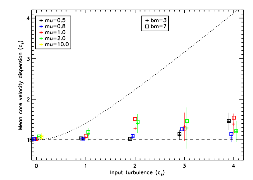
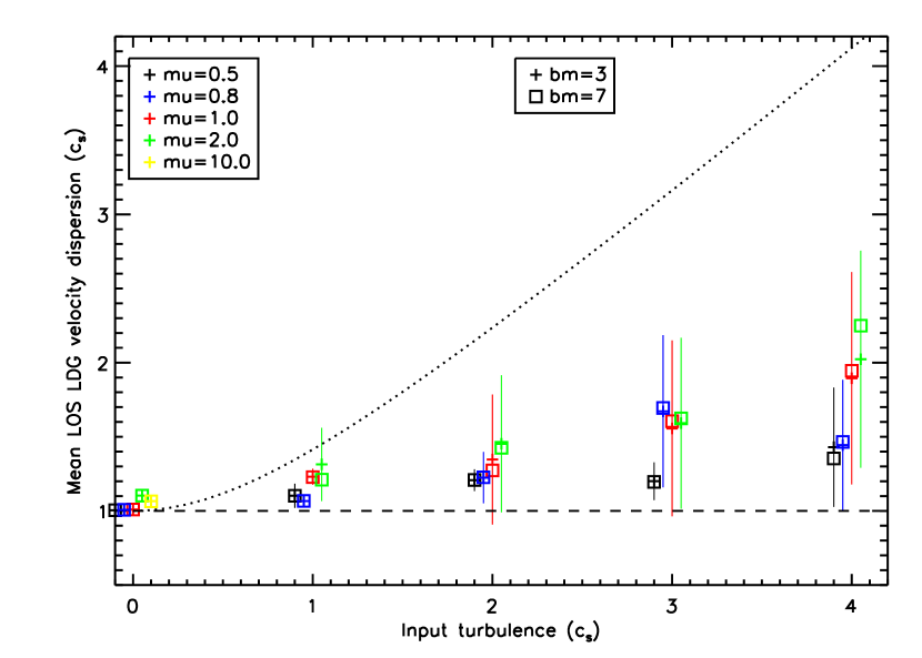
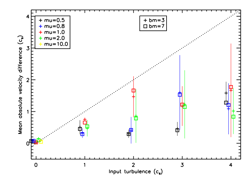
We first re-analyze the simulations using a larger beamsize (in pixels) with everything else identical to our standard method. Assuming a mean density $\sim$5 times higher than our nominal value and keeping the other constants fixed, for example, would shrink the physical size of each pixel and thus the beamsize would change to 7 pixels for N₂H⁺ (and 3 pixels for C¹⁸O). The observable quantities which we are interested in are the velocity dispersion of the core and LOS LDG material and the relative motion of the core and LOS LDG material. It would be difficult to compare these quantities on a core-to-core basis, since different cores could be identified in each (a larger beamsize increases the minimum separation required between cores). Instead, we use the mean and standard deviation of these quantities to represent the full span of values found for each simulation. (We use the absolute value for the relative motion of the core and LOS LDG material.)

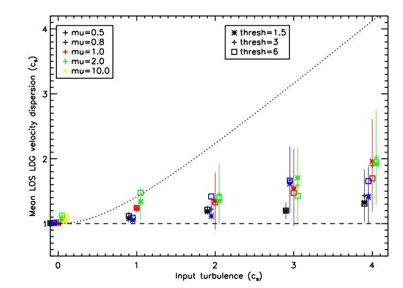
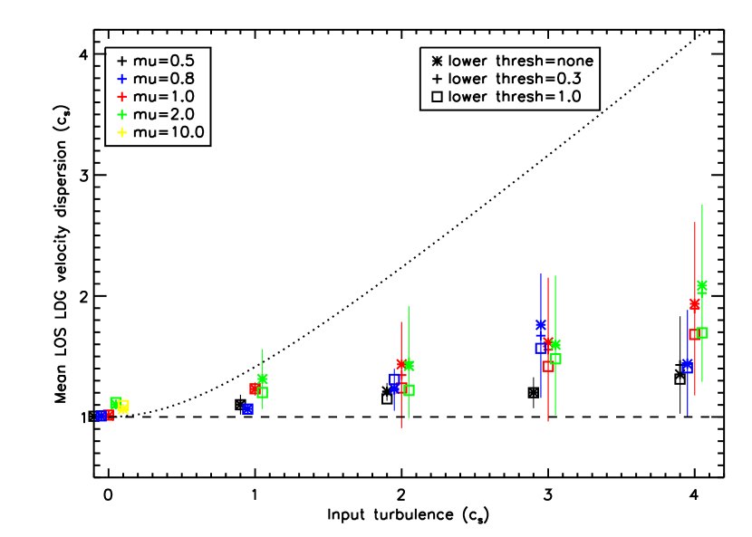
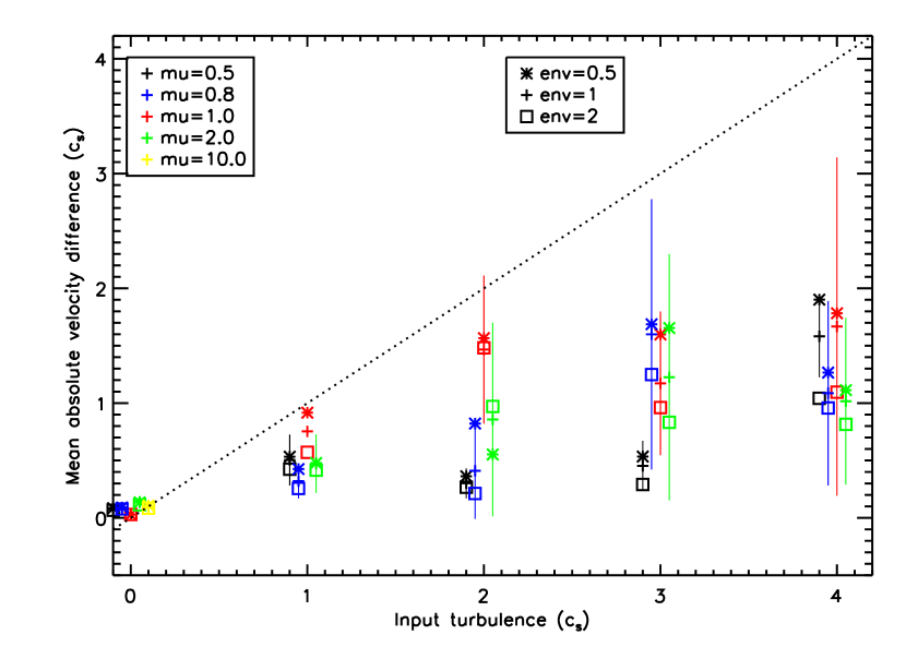
Figures 21, 22, and 23 (left hand panels) show the variation of ‘observables’ (the core velocity dispersion, LOS LDG velocity dispersion, and core to LOS LDG velocity difference) versus the velocity dispersion of the region as a whole for the nominal beamsize (plus signs) and the larger beamsize (squares). In most cases, the larger beamsize has relatively little effect on the ‘observables’.

The highly turbulent simulations tend to display filamentary structure in the 2D column density, which translates to clustered peaks in the 1D projected column density distribution which we use to identify cores. A larger beamsize tends to slightly decrease the number of cores identified, particularly in the highly turbulent simulations. The filamentary structure also leads to a larger amount of higher (column) density material in the core’s vicinity; hence the core velocity dispersion in particular, and the LOS LDG velocity dispersion to a lesser extent tend to increase with an increasing beamsize, while the core-to-LOS LDG motion is less affected.

The fraction of mass in dense cores and number of cores detected (not plotted) show little to no variation with the varying beamsize, with differences in values no more than a few percent of the mass and one or two in number of cores.

A.3 Core Threshold

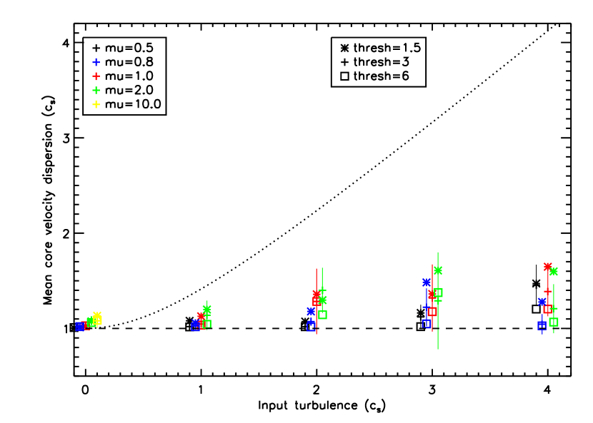
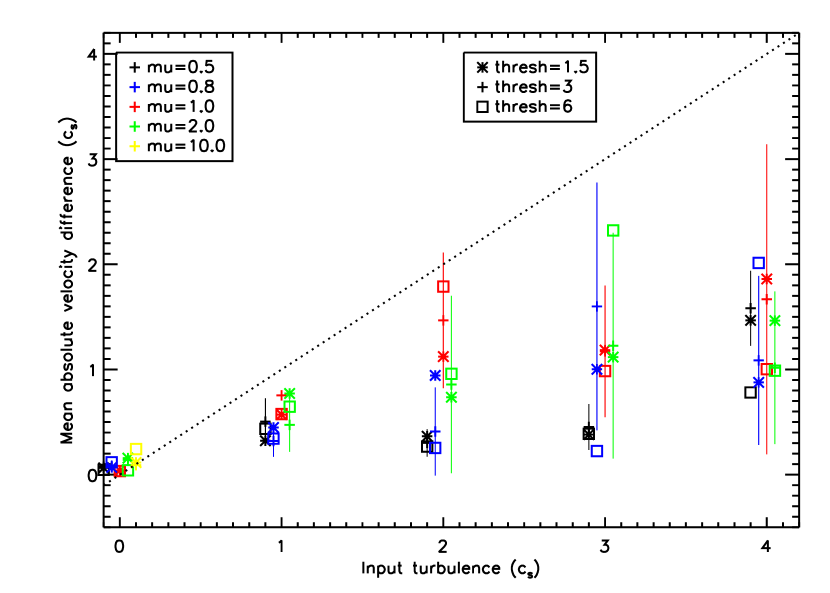
We next re-analyze the data using a higher and lower minimum core column density threshold (relative to the mean). A lower chosen physical mean density, for example, would require a higher minimum core column density relative to the mean in order to keep the same absolute value. The simulations have a relatively small dynamic range (less than two orders of magnitude in column density), so we test a minimum core column density threshold of twice and half our nominal value (i.e., 6 and 1.5 times the mean).

Figures 21, 22, and 23 (right hand panels) show the effect of varying the core identification threshold using the same plotting scheme as the left hand panels described above. As is found for the beamsize, the majority of ‘observables’ do not vary significantly with a different core identification threshold. As is also found for the variation in beamsize, the fraction of mass in the cores varies at most by a few percent and the number of cores varies by at most a few.

The greatest effect of a higher core identification threshold is that fewer cores are identified. As mentioned above, the dynamic range of the simulations is not large (the simulations are stopped when the peak column density exceeds roughly 10 times the mean), hence even the factor of two increase in the minimum core column density can significantly reduce the number of cores identified, in many cases to only one or two cores per simulation. The very small number statistics drawn from this appears to be the largest contributor to the variations seen between the two thresholds.

At the lower core identification threshold, more cores are identified, although usually not substantially more than the nominal case. Here, the main differences originate from a larger fraction of material being included as part of the ‘core’ and a smaller fraction as the ‘LOS LDG’. The amount of material excluded from the LOS LDG is a small fraction of the total, hence the LOS LDG velocity dispersions tend to decrease by only a small amount. This material makes up a larger fraction of the total core mass, hence the increase in core velocity dispersions tend to be somewhat larger. There is no obvious trend in the relative motions determined.

A.4 LOS LDG Upper Threshold

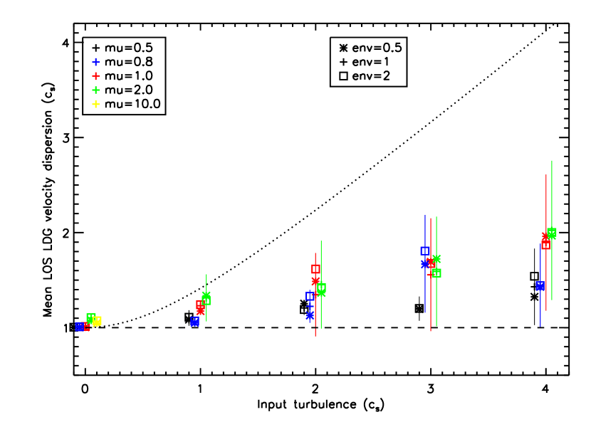
The other physical property which plays an implicit rather than explicit role is a chemical one – the density range in which N₂H⁺ and C¹⁸O are sensitive. The minimum density at which N₂H⁺ is sensitive sets the value for the core identification threshold and folds into the core identification threshold discussed above. The maximum density before C¹⁸O becomes significantly depleted sets the threshold for which material is considered to contribute to our LOS LDG measures. We nominally consider these two values to be identical, so that all of the material in the simulation is traced either by N₂H⁺ or C¹⁸O, but this might not be the case. Here, we consider cases where C¹⁸O is sensitive to half and twice the minimum density for N₂H⁺ emission.

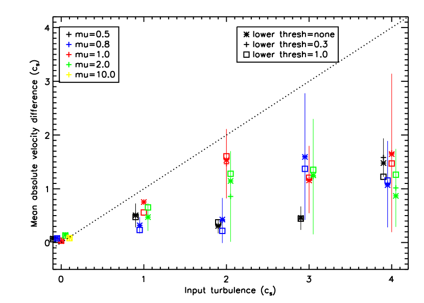
The left hand panels of Figures 24 and 25 show the LOS LDG velocity dispersion (Figure 24) and core to LOS LDG velocity difference (Figure 25) versus the velocity dispersion of the region as a whole for three different maximum C¹⁸O threshold values. (Note the core velocity dispersion remains unchanged, hence is not shown.) The change in LOS LDG column density threshold has little effect on the LOS LDG velocity dispersion (Figure 24), as one would expect given that most of the mass is found at the lower column densities which are included in all cases. There is a slightly larger change in the core-to-LOS LDG motion since the higher column density material tends to have a similar velocity to that of core material. Although the width of the spectral feature is little affected by the inclusion of higher column density material in the LOS LDG spectrum, the position of the peak tends to be pushed towards velocities nearer to that of the core. This is clearly illustrated in Figure 25 which shows the lower LOS LDG column density threshold results in larger relative core-to-LOS LDG motions while a higher threshold leads to smaller relative motions. While the change in the core-to-LOS LDG motion is larger than the change in the LOS LDG velocity dispersion, both changes are relatively small. This result could have been anticipated from the brief discussion in Section 4.3 and Figure 6, where it was demonstrated that the LOS LDG spectra look very similar to the spectrum that would result from contributions due to all of the material along the line of sight, since only a small fraction of the material has high column density.

A.5 LOS LDG Lower Threshold

Like any molecular tracer, C¹⁸O also has a minimum density to which it is sensitive. In our analysis above, we assume that the minimum density reached in the simulation is sufficiently high that C¹⁸O will trace all of of the low density material, but this might not be the case. Here, we consider cases where C¹⁸O is sensitive to only material above one third and one times the mean column density while keeping the maximum column density the same as our standard analysis (three times the mean column density).

The right hand panels of Figures 24 and 25 show the LOS LDG velocity dispersion (Figure 24) and core to LOS LDG velocity difference (Figure 25) versus the velocity dispersion of the region as a whole for three different maximum C¹⁸O threshold values. (Note the core velocity dispersion remains unchanged, hence is not shown.) The change in the minimum LOS LDG column density has little effect on the LOS LDG velocity dispersion, except in a few of the highly turbulent simulations where the LOS LDG velocity dispersion becomes somewhat lower when only material between one and three times the mean column density is considered. Similarly, the change in the core to LOS LDG motion calculated using different minimum LDG column density thresholds is small, with higher thresholds tending to slightly reduce the velocity difference. This illustrates the fact that most of the mass in the simulations is at moderately low column densities and that even using a greatly reduced range of column densities for the LOS LDG calculations has very little effect on our results.

Appendix B RESOLUTION

As discussed in §2.1, the simulations we analyze here have 128 by 128 cells, in order for a large parameter study to be performed. To test whether resolution influenced the results of our calculations, we have also analyzed a subset of four times higher linear resolution models (512 by 512 cells). The results show that the original simulations are sufficient for our purposes. Here, we demonstrate that our results are not affected by the resolution adopted. We analyzed additional simulations with a Mach number of 4 and both weak ($\mu_{0}=2$) and strong ($\mu_{0}=0.5$) magnetic fields. The high Mach number simulations are the most likely to be affected by resolution since stronger turbulence has a greater ability to compress material to smaller scales.

We computed all of the ‘observable’ properties of the two additional simulations and found them to be consistent with their lower-resolution simulation counterparts. Tables 6 and 7 show the mean and standard deviation of the ‘observables’ analyzed in the paper at both the original and high resolution. As can be seen from these tables, there is no obvious change in any of the observables due to the higher resolution used. Note that identical results for the higher resolution simulations are not expected because the initial random distribution of turbulent velocities is different for each simulation run. Initial conditions, and in particular how these influence the time at which the simulation reaches a factor of 10 in column overdensity, have a much larger effect on the results than the change in resolution.

Table 1: Properties of Extinction Regions.

Number	Mass	Radius	$\sigma V_{grav}$	$\sigma V_{CO}$	Coverage	Notes
	(M⊙)	(′)	(km s-1)	(km s-1)	(%)
1	859.6	12.9	0.89	0.62	100	B5
2	1938.9	18.7	1.11	0.91	100	IC348
3	780.6	12.3	0.87	1.03	96	SW of IC348
4	560.5	11.2	0.77	0.94	56	E of B1
5	441.1	9.7	0.73	0.87	100	B1
6	257.6	7.6	0.63	0.87	52	SW of B1
7	973.3	14.8	0.88	1.22	100	NGC1333
8	246.2	7.6	0.62	0.83	100	S of NGC1333
9	240.1	7.5	0.62	0.87	40	L1455
10	173.7	6.4	0.56	0.79	100	L1448
11	107.4	5.2	0.50	0.76	84	S of L1448

Table 2: Observed Core Formation Statistics

Ext #	$\sigma V_{tot}/c_{S}$	$N_{C,SCUBA}$	$N_{C,tot}$	CFEC,SCUBA	CFEC,tot
1	2.9	2	8	0.1	0.7
2	4.1	11	19	0.7	1.0
3	4.6	0	2	0.0	0.2
5	3.9	7	17	3.1	5.0
7	5.4	26	27	5.0	5.1
8	3.7	0	0	0.0	0.0
10	3.5	5	7	8.0	9.0
11	3.4	0	2	0.0	1.6

Table 3: Simulation Timescales.

$M$			Time ($t_{0}$)
($c_{s}$)	$\mu_{0}=0.5$	$\mu_{0}=0.8$	$\mu_{0}=1.0$	$\mu_{0}=2.0$	$\mu_{0}=10$
0	204	167	121	23	12
1	49.6	31.6	4.3	2.5	–
2	28.7	10.8	2.5	1.1	–
3	36.0	0.9	0.8	0.8	–
4	2.1	1.0	0.7	0.5	–

Table 4: Simulation Dynamic Observables

$M$	$\mu_{0}$	Projection	$\sigma V_{LOSLDG,all}$		$\sigma V_{LOSLDG,cores}$		$\sigma V_{core}$		Core to LOS LDG
			mean	stddev	mean	stddev	mean	stddev	mean	stddev
0	0.5	X	1.00	0.00	1.00	0.00	1.00	0.00	0.07	0.05
0	0.5	Y	1.00	0.00	1.00	0.00	1.00	0.01	0.08	0.06
1	0.5	X	1.10	0.10	1.12	0.13	1.03	0.03	0.40	0.34
1	0.5	Y	1.07	0.05	1.09	0.04	1.01	0.00	0.58	0.05
2	0.5	X	1.12	0.06	1.16	0.01	1.02	0.00	0.23	0.01
2	0.5	Y	1.17	0.11	1.29	–	1.02	–	0.45	–
3	0.5	X	1.24	0.19	1.25	0.16	1.17	0.15	0.38	0.05
3	0.5	Y	1.13	0.07	1.13	0.02	1.05	0.03	0.55	0.34
4	0.5	X	2.22	0.43	1.37	0.32	1.34	0.13	1.68	0.22
4	0.5	Y	1.95	0.83	1.54	0.55	1.68	0.17	1.39	0.61
0	1.0	X	1.00	0.00	1.01	0.00	1.02	0.03	0.02	0.01
0	1.0	Y	1.00	0.00	1.01	0.01	1.03	0.03	0.04	0.04
1	1.0	X	1.08	0.07	1.19	–	1.07	–	0.74	–
1	1.0	Y	1.16	0.11	1.27	–	1.03	–	0.76	–
2	1.0	X	1.85	0.54	1.17	0.31	1.23	0.33	1.48	0.13
2	1.0	Y	1.73	0.49	1.49	0.50	1.34	0.42	1.46	1.01
3	1.0	X	2.59	0.97	1.77	0.76	1.16	0.16	1.06	0.69
3	1.0	Y	2.18	0.37	1.31	0.14	1.52	0.45	1.31	0.60
4	1.0	X	3.28	0.97	2.09	0.90	1.48	0.26	1.35	1.02
4	1.0	Y	3.00	0.81	1.70	0.44	1.31	0.25	1.95	1.80
0	2.0	X	1.06	0.04	1.10	–	1.05	–	0.17	–
0	2.0	Y	1.04	0.03	1.10	0.00	1.10	0.05	0.13	0.00
1	2.0	X	1.55	0.22	1.35	0.34	1.23	0.18	0.36	0.23
1	2.0	Y	1.34	0.09	1.27	0.08	1.05	0.04	0.58	0.26
2	2.0	X	1.92	0.73	1.61	0.54	1.32	0.25	0.63	0.99
2	2.0	Y	1.86	0.21	1.22	0.18	1.56	0.15	1.32	0.04
3	2.0	X	3.17	0.52	1.64	0.70	1.14	0.15	1.07	1.03
3	2.0	Y	2.41	0.65	1.50	0.22	1.60	0.84	1.54	1.24
4	2.0	X	3.02	0.70	2.14	1.02	1.52	0.14	1.46	0.90
4	2.0	Y	3.17	0.76	1.96	0.57	1.08	0.17	0.84	0.61
0	10.0	X	1.04	0.02	1.08	0.03	1.10	0.09	0.09	0.04
0	10.0	Y	1.03	0.03	1.05	0.03	1.06	0.07	0.09	0.06
0	0.8	X	1.00	0.00	1.02	–	1.04	–	0.11	–
0	0.8	Y	1.00	0.00	1.00	0.00	1.01	0.01	0.07	0.06
1	0.8	X	1.03	0.01	1.05	0.03	1.02	0.01	0.29	0.21
1	0.8	Y	1.05	0.05	1.08	0.05	1.03	0.03	0.34	0.15
2	0.8	X	1.37	0.24	1.16	0.20	1.09	0.07	0.54	0.73
2	0.8	Y	1.20	0.13	1.29	0.14	1.06	0.03	0.32	0.23
3	0.8	X	2.75	0.45	1.64	0.35	1.11	0.11	1.87	1.25
3	0.8	Y	2.25	0.66	1.72	0.75	1.45	0.08	1.06	1.00
4	0.8	X	2.75	0.44	1.48	0.52	1.05	0.09	0.89	0.99
4	0.8	Y	2.22	0.49	1.41	0.38	1.04	0.13	1.24	0.64

Table 5: Simulation Core Formation Statistics

$M$	$\sigma V_{box}$	$\mu_{0}$	Projection	$N_{C}$	$CFE_{C}$
0	1.0	0.5	X	3	1.1
0	1.0	0.5	Y	0	0.0
1	1.2	0.5	X	3	1.9
1	1.1	0.5	Y	1	0.0
2	1.7	0.5	X	2	0.9
2	1.3	0.5	Y	1	0.2
3	2.1	0.5	X	4	4.0
3	1.3	0.5	Y	2	0.9
4	2.7	0.5	X	4	2.8
4	3.7	0.5	Y	2	1.4
0	1.0	1.0	X	2	0.9
0	1.0	1.0	Y	0	0.0
1	1.3	1.0	X	1	2.8
1	1.2	1.0	Y	0	0.0
2	1.9	1.0	X	2	1.6
2	1.8	1.0	Y	1	0.1
3	3.2	1.0	X	4	2.8
3	3.3	1.0	Y	2	1.6
4	3.5	1.0	X	5	4.9
4	3.6	1.0	Y	4	2.7
0	1.1	2.0	X	1	0.6
0	1.0	2.0	Y	1	0.3
1	1.6	2.0	X	4	2.3
1	1.5	2.0	Y	1	0.4
2	2.1	2.0	X	4	3.0
2	2.5	2.0	Y	1	0.4
3	3.6	2.0	X	6	3.9
3	3.3	2.0	Y	2	0.4
4	4.3	2.0	X	4	1.3
4	4.1	2.0	Y	3	0.5
0	1.0	10.0	X	5	1.6
0	1.0	10.0	Y	1	0.3
0	1.0	0.8	X	1	0.6
0	1.0	0.8	Y	1	0.1
1	1.1	0.8	X	2	1.2
1	1.3	0.8	Y	0	0.0
2	1.7	0.8	X	2	1.8
2	1.4	0.8	Y	0	0.0
3	2.9	0.8	X	4	2.0
3	3.2	0.8	Y	1	0.1
4	4.4	0.8	X	5	2.0
4	4.0	0.8	Y	4	0.6

Table 6: Comparison Between $\mu_{0}=2.0$, Mach 4 Simulations

	N=128		N=512
Quantity	Mean	Std Dev	Mean	Std Dev
Region Velocity Dispersion	4.24	0.14	4.21	0.04
All LOS Vel Disp X (matching 13CO observations)	2.90	0.94	2.66	0.62
All LOS Velocity Dispersion Y Projection	3.28	1.16	2.64	0.65
LOS Vel Disp where Cores (matching C18O observations)	2.02	0.73	1.89	0.67
Core Velocity Dispersion	1.21	0.26	1.26	0.41
Absolute Core-LOS Vel Difference	1.02	0.73	2.04	1.19
Absolute Core-LOS Vel Diff / LOS Vel Disp	0.49	0.34	0.92	0.45
Absolute Core Velocities	2.23	2.07	3.54	2.27
Number of Cores	3.5	0.7	6.5	2.1
Percentage of Mass in Cores	0.9	0.5	0.5	0.6

Table 7: Comparison Between $\mu_{0}=0.5$, Mach 4 Simulations

	N=128		N=512
Quantity	Mean	Std Dev	Mean	Std Dev
Region Velocity Dispersion	3.17	0.71	3.90	0.73
All LOS Vel Disp X (matching 13CO observations)	2.27	0.57	2.85	1.11
All LOS Velocity Dispersion Y Projection	1.96	0.79	2.16	0.92
LOS Vel Disp where Cores (matching C18O observations)	1.43	0.40	1.53	0.33
Core Velocity Dispersion	1.45	0.22	1.28	0.21
Absolute Core-LOS Vel Difference	1.58	0.36	1.90	1.32
Absolute Core-LOS Vel Diff / LOS Vel Disp	1.09	0.33	0.91	0.27
Absolute Core Velocities	1.91	1.24	2.01	1.53
Number of Cores	2.5	1.4	3.0	0.0
Percentage of Mass in Cores	2.1	1.0	1.4	1.0

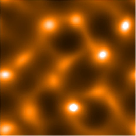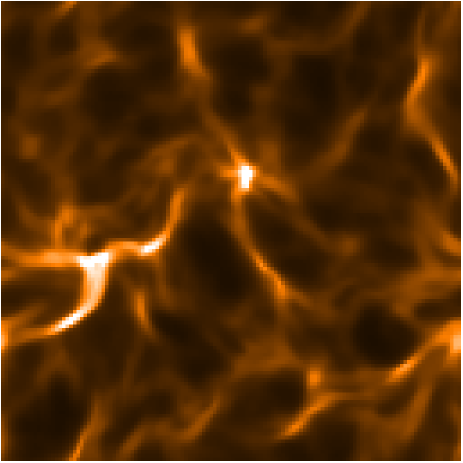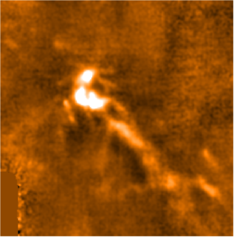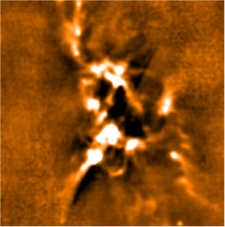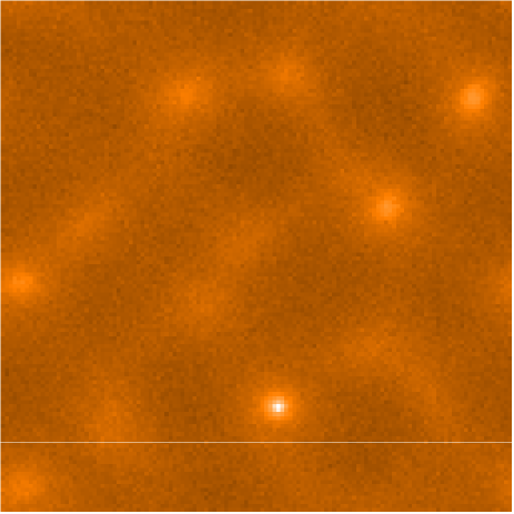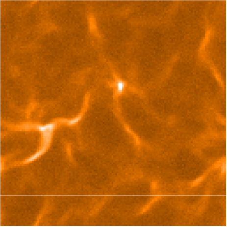Figure 1: The final column density in two simulations – with $\mu_{0}=0.5,M=0$ (left) and $\mu_{0}=1.0,M=3$ (right). The scale, in units of the initial column density, is shown in the bar. Under the scalings we applied, a value of 1 corresponds to 3.5$\times 10^{21}$ cm^-2.

Figure 2: SCUBA submillimetre maps of two well-known star forming regions – B1 and NGC1333. Each image spans 21′ ($\sim$1.5 pc) and the scale bar is in units of Jy bm^-1.

Figure 3: The same simulations shown in Figure 1, with the column density converted to equivalent SCUBA flux. White noise has been added at approximately the same level as the noise in the SCUBA observations. The linear size and scale bar are the same as in Figure 2.

Figure 4: Projected 1D column density distribution (in the x direction) for the simulations shown in Figure 1 ($\mu_{0}=0.5$, $M=0$ on the left and $\mu_{0}=1.0$, $M=3$ on the right). Using our assumed scalings, a 1D column density value of 100 corresponds to $3.5\times 10^{23}$ cm^-1. Cores are identified as peaks above a specified threshold and separated by at least three pixels corresponding to roughly 29″or one IRAM N₂H⁺ beam. The dashed horizontal line indicates the mean projected column density while the dotted horizontal line indicates the threshold for core identification. The solid horizontal lines indicate the extent of each core identified while the solid and dotted vertical lines indicate the core centres and width respectively.

Figure 5: Two examples of spectra calculated for the core and LOS LDG material. The solid lines show the calculated (‘observed’) spectra while the dashed and dotted lines show the model (Gaussian) spectral fit. The top panels show the core spectra while the bottom panels show the LOS LDG material spectra. The left figure shows an example from a non-turbulent simulation with a subcritical mass to magnetic flux ratio ($\mu_{0}=0.5$, $M=0$) where the spectra are well-described by a single Gaussian. The right figure shows an example from a highly turbulent simulation with a critical mass to flux ratio ($\mu_{0}=1$, $M=3$) where the LOS LDG spectrum is less well-fit by even a two Gaussians.

Figure 6: The spectrum calculated for a core identified in a simulation with a subcritical mass to magnetic flux ratio ($\mu_{0}$=0.8) and high input turbulence ($M$=3). This core was found to have supersonic motion between the core and LOS LDG material. The top panel shows the normalized spectrum of the core, with the best fit Gaussian shown by the dashed line (the fit parameters are given in the legend). The middle panel shows the normalized spectrum for the LOS LDG material around the core, with the two Gaussian fits indicated by the dashed lines. The lowest panel shows the normalized spectrum that would have been calculated for the LOS LDG material had all of the material along the LOS been used (rather than excluding that above the core detection threshold), as well as the core spectrum multiplied by a factor of five for visibility. There is little difference between this spectrum and the one used in our analysis (middle panel), indicating that our analysis is little effected by the inclusion of the core material in the LOS LDG spectrum (as also discussed in §4.3).

Figure 7: Calculated ¹³CO spectra for one of the LOS’s in the most turbulent simulation, with the weakest magnetic field ($\mu$=2) and highest input turbulence ($M=4$). The spectrum’s amplitude has been normalized to the maximum intensity. The dotted horizontal lines indicate the extent of the spectrum at half- and quarter- maximum intensity. Note how it is necessary to measure the width well below the half-maximum mark in order to be sensitive to low-lying large scale modes.

Figure 8: The velocity dispersion of the material in the entire simulated region measured at the end of the simulation versus the input level of turbulence. The dashed line indicates a thermal velocity dispersion while the dotted line shows the relationship for a velocity dispersion equal to the input turbulence. Squares and plusses show the results for the x and y projections of the simulations respectively. The simulations with strong magnetic fields show much smaller velocity dispersions than would be expected from the original input turbulence.

Figure 9: The velocity dispersion of low density material (¹³CO ) measured along the central chord through each extinction region versus the velocity dispersion seen across the region as a whole. The filled symbols indicate regions where star formation is more recent, while the shading indicates the region spanned by these observations.

Figure 10: The velocity dispersion of low density material measured along all lines of sight in the simulation versus the velocity dispersion in the region as a whole. The shading indicates the region spanned by the observations (see Figure 9).

Figure 11: The velocity dispersion of low density material (C¹⁸O) versus the velocity disperison measured in the larger extinction region (diamonds). The solid vertical lines indicate the range of velocity dispersions through the central chord of each extinction region, while the asterisk indicates the mean velocity dispersion. The dotted line indicates a 1-1 relationship while the dashed lines indicate thermal objects. The filled symbols indicate regions where star formation is more recent. The shaded region represents roughly the area spanned by our observations.

Figure 12: The velocity dispersion of low density material in the simulations versus the total velocity dispersion observed in the region (plus signs). The solid vertical lines indicate the full range of velocity dispersions that are seen along all lines of sight in the region within a ‘beamsize’ matching that of the ¹³CO observations. The shaded region represents roughly the area spanned by our observations (see Figure 11).

Figure 13: The internal velocity dispersion of the cores versus the velocity dispersion of their large-scale environment. The filled symbols indicate regions where star formation is more recent. The shaded region represents roughly the area spanned by our observations.

Figure 14: The internal velocity dispersion of the cores versus the velocity dispersion of their large-scale environment for the simulations. The shaded region represents roughly the area spanned by our observations (see Figure 13).

Figure 15: The observed relative motions of the core and its surrounding LOS LDG material versus the velocity dispersion of the extinction region. The filled symbols indicate regions where star formation is more recent. The shaded region represents roughly the area spanned by our observations.

Figure 16: The relative motions of the core and its surrounding LOS LDG material in the simulations versus the velocity dispersion of the region. The shaded region represents roughly the area spanned by our observations (see Figure 15).

Figure 17: The ratio of observed core to LOS LDG motion and LOS LDG velocity dispersion versus the velocity dispersion of the extinction region. The dash-dot line indicates the point at which cores move faster than the velocity dispersion of the LOS LDG with respect to their local environment (see §5.2). The filled symbols indicate regions where star formation is more recent. The shaded region represents roughly the area spanned by observations.

Figure 18: The ratio of core to LOS LDG motion and LOS LDG velocity dispersion in the simulation versus the velocity dispersion of the entire region. The dash-dot line indicates the line at which cores move faster than the velocity dispersion of the LOS LDG with respect to their local environment (see §5.2). The shaded region represents roughly the area spanned by our observations (see Figure 17).

Figure 19: The motion of the observed N₂H⁺ cores in Perseus within their parent extinction regions versus the velocity dispersion of the extinction regions they inhabit (as measured in ¹³CO ). The dotted line indicates a 1-1 relation. The filled symbols indicate regions where star formation is more recent. The shaded region represents roughly the area spanned by our observations.

Figure 20: The difference between core and region centroid velocity versus the velocity dispersion of the region for the simulations. The dotted line indicates a 1-1 relation. The shaded region represents roughly the area spanned by our observations (see Figure 19).

Figure 21: The variation in core velocity dispersion for cores identified with a differing beamsize (left) and minimum core column density threshold (right) versus the input turbulence. The plus signs and vertical lines indicate the mean and standard deviation of the velocity dispersion found for each simulation using our nominal values. The squares and asterisks indicate the mean found for the simulations with a differing beamsize (left) or core threshold (right). Note the data points have been slightly offset from the input turbulence to allow better visibility.

Figure 22: The variation in LOS LDG velocity dispersion for cores identified with a differing beamsize (left) and minimum core colum density threshold (right) versus the input turbulence. See Figure 21 for the plotting conventions used.

Figure 23: The variation in core to LOS LDG velocity difference for cores identified with differing beamsize (left) and minimum core column density threshold (right) versus the input turbulence. See Figure 21 for the plotting conventions used.

Figure 24: The variation in LOS LDG velocity dispersion for a differing LDG column density range. The left hand panel shows the effect of changing the maximum LDG column density threshold while the right hand panel shows the effect of changing the minimum LDG column density threshold. See Figure 21 for the plotting conventions used.

Figure 25: The variation in absolute core to LOS LDG velocity difference for a differing LDG column density range. The left hand panel shows the effect of changing the maximum LDG column density threshold while the right hand panel shows the effect of changing the minimum LDG column density threshold. See Figure 21 for the plotting conventions used.

References

- André, Ward-Thompson, & Barsony (1993) André, P., Ward-Thompson, D., & Barsony, M. 1993, ApJ, 406, 122
- André & Saraceno (2005) André, P. & Saraceno, P. 2005, Proceedings of the dusty and molecular universe: a prelude to Herschel and ALMA, A. Wilson (eds), ESA Publications, Noordwijk, Netherlands, p179-184
- Ayliffe et al. (2007) Ayliffe, B. A., Langdon, J. C., Cohl, H. S., & Bate, M.R. 2007, MNRAS, 374, 1198
- Ballesteros-Paredes et al. (2003) Ballesteros-Paredes, J. Klessen, R. S. & Vázquez-Semadeni, E. 2003, ApJ, 592, 188
- Basu & Ciolek (2004) Basu, S. & Ciolek, G. E. 2004, ApJ, 607, 39L
- Basu, Ciolek & Wurster (2009) Basu, S., Ciolek, G. E., & Wurster, J. 2009, NewA, 14, 221
- Basu, Ciolek, Dapp & Wurster (2009) Basu, S., Ciolek, G. E., Dapp, W. B. & Wurster, J. NewA, 14, 483
- Benson & Myers (1989) Benson, P. J. & Myers, P. C. 1989, ApJS, 71, 89
- Bonnell, Larson, & Zinnecker (2007) Bonnell, I. A., Larson, R. B., Zinnecker, H. 2007, Protostars and Planets V, B. Reipurth, D. Jewitt, & K. Keil (eds), University of Arizona Press, Tuscon, p149-164
- Burkert & Hartmann (2004) Burkert, A. & Hartmann, L. 2004, ApJ, 616, 288
- ernis (1993) ernis, K. 1993, BaltA, 2, 214
- Ciolek & Basu (2006) Ciolek, G. E. & Basu, S. 2006, ApJ, 652, 442
- Di Francesco et al. (2007) Di Francesco, J., Evans, N. J. II, Caselli, P., Myers, P. C., Shirley, Y., Aikawa, Y., Tafalla, M. 2007, Protostars and Planets V, B. Reipurth, D. Jewitt, & K. Keil (eds), University of Arizona Press, Tuscon, p17-32
- Elmegreen (2007) Elmegreen, B. G. 2007, ApJ, 668, 1064
- Gammie & Ostriker (1996) Gammie, C. F. & Ostriker, E. C. 1996, ApJ, 466, 814
- Hatchell et al. (2005) Hatchell, J., Richer, J. S., Fuller, G. A., Qualtrough, C. J., Ladd, E. F., & Chandler, C. J. 2005, A&A, 440, 151
- Henriksen et al. (1997) Henriksen, R., André, P., & Bontemps, S. 1997, A&A, 323, 549
- Jijina et al. (1999) Jijina, J., Myers, P. C., Adams, F. C. 1999, ApJS, 125, 161
- Johnstone, Di Francesco & Kirk (2004) Johnstone, D., Di Francesco, J., & Kirk, H. 2004, ApJ, 611, 45L
- Jørgensen et al. (2008) Jørgensen, J. K., Johnstone, D., Kirk, H., Myers, P. C., Allen, L., Shirley, Y. 2008, ApJ, 683, 822
- Jørgensen et al. (2007) Jørgensen, J. K., Johstone, D., Kirk, H., & Myers, P. C. 2007, ApJ, 656, 293
- Kirk, Johnstone & Di Francesco (2006) Kirk, H., Johnstone, D. & Di Francesco, J. 2006, ApJ, 646, 1009
- Kirk, Johnstone & Tafalla (2007) Kirk, H., Johnstone, D. & Tafalla, M. 2007, ApJ, 668, 1042
- Klessen et al. (2005) Klessen, R. S., Ballesteros-Paredes, J., Vázquez-Semadeni, E., Duran-Rojás, C. 2005, ApJ, 620, 786
- Kudoh & Basu (2008) Kudoh, T., Basu, S. 2008, ApJ, 679, L97
- Lada (1987) Lada, C. J. 1987, Proceedings of the Symposium, Tokyo, Japan, Dordrecht, D. Reidel Publishing Co., p1-17
- Lada & Lada (2003) Lada, C. J. & Lada, E. A. 2003, ARA&A, 41, 57
- Larson (1981) Larson, R. B. 1981, MNRAS, 194, 809
- Li & Nakamura (2004) Li, Z.-Y., & Nakamura, F. 2004, ApJ, 609, L83
- Lombardi & Alves (2001) Lombardi, M. & Alves, J. 2001, A&A, 337, 1023
- MacLow & Klessen (2004) MacLow, M-M. & Klessen, R. 2004, RvMP, 76, 125
- Offner et al. (2008) Offner, S. S. R., Klein, R. I., & McKee, C. F. 2008, AJ, 136, 404
- Onishi et al. (1998) Onishi, T., Mizuno, A., Kawamura, H. O., & Fukui, Y. 1998, ApJ, 502, 296
- Rosolowsky et al. (2008) Rosolowsky, E. W., Pineda, J. E., Foster, J. B., Borkin, M. A., Kauffmann, J., Caselli, P., Myers, P. C., Goodman, A. A. 2008, ApJS, 175, 509
- Ridge et al. (2006) Ridge, N. A., Di Francesco, J., Kirk, H., Li, D., Goodman, A. A., Arce, H. G., Borkin, M. A., Caselli, P., Foster, J. B., Heyer, M. H., Johnstone, D., Kosslyn, D. A., Lombardi, M., Pineda, J. E., Schnee, S. L., & Tafalla, M. 2006, AJ, 131, 2921
- Shu et al. (1994) Shu, F., Najita, J.,Ostriker, E., Wilkin, F., Ruden, S., & Lizano, S. 1994, ApJ, 429, 781
- Stahler & Palla (2004) Stahler, S. W. & Palla, F. 2004, The Formation of Stars (Wiley-Vch)
- Tafalla et al. (2002) Tafalla, M., Myers, P. C., Caselli, P., Walmsley, C. M., Comito, C. 2002, ApJ, 569, 815
- Terebey et al. (1984) Tereby, S., Shu, F. H., & Cassen, P. 1984, ApJ, 286, 529
- Ungerechts et al. (1997) Ungerechts, H., Bergin, E. A., Goldsmith, P. F., Irvine, W. M., Schloerb, F. P. & Snell, R. L. 1997, ApJ, 482, 245
- Walsh et al. (2004) Walsh, A. J., Myers, P. C. & Burton, M. G. 2004, ApJ, 614, 194
- Walsh et al. (2007) Walsh, A. J., Myers, P. C., Di Francesco, J., Mohanty, S., Bourke, T. L., Gutermuth, R., & Wilner, D. 2007, ApJ, 655, 958
- Ward-Thompson et al. (2007) Ward-Thompson, D., André, P., Crutcher, R., Johnstone, D., Onishi, T., & Wilson, C. 2007, Protostars and Planets V, B. Reipurth, D. Jewitt, & K. Keil (eds), University of Arizona Press, Tuscon, p33-46
- Ward-Thompson et al. (2007b) Ward-Thompson, D., et al. 2007, PASP, 119, 855