Accurate image reconstruction from few-views and limited-angle data in divergent-beam CT

Abstract

In practical applications of tomographic imaging, there are often challenges for image reconstruction due to under-sampling and insufficient data. In computed tomography (CT), for example, image reconstruction from few views would enable rapid scanning with a reduced x-ray dose delivered to the patient. Limited-angle problems are also of practical significance in CT. In this work, we develop and investigate an iterative image reconstruction algorithm based on the minimization of the image total variation (TV) that applies to divergent-beam CT. Numerical demonstrations of our TV algorithm are performed with various insufficient data problems in fan-beam CT. The TV algorithm can be generalized to cone-beam CT as well as other tomographic imaging modalities.

I Introduction

In various forms of tomography, one of the main issues for image reconstruction centers on data sufficiency and on how to estimate a tomographic image when the projection data are not theoretically sufficient for exact image reconstruction. Insufficient data problems occur quite frequently because of practical constraints due to the imaging hardware, scanning geometry, or ionizing radiation exposure. The insufficient data problem can take many forms, but the forms that we shall consider in this work relate to divergent-beam x-ray computed tomography (CT). One aspect of the insufficient data problem derives from sparse samples; namely, we will consider image reconstruction from projection data at few views. We will also consider two other imperfect scanning data situations: limited angular range and gaps in the projection data caused by bad detector bins. In each of these three examples, the projection data are not sufficient for exact reconstruction of tomographic images and application of standard analytic algorithms such as filtered back-projection (FBP) will lead to conspicuous artifacts in reconstructed images.

There have been a number of algorithms proposed to overcome data insufficiency in tomographic imaging, and there are essentially two types of approaches. First, one can interpolate or extrapolate the missing data regions from the measured data set, followed by analytic reconstruction. Such approaches may be useful for a specific scanning configuration, imaging a particular object. It is, however, difficult to make general conclusions on the utility of such an approach. Second, one can employ an iterative algorithm to solve the data model for images from the available measurements. Numerous iterative algorithms have been used for tomographic image reconstruction with varying degrees of success. These algorithms differ in the constraints that they impose on the image function, the cost function that they seek to minimize, and the actual implementation of the iterative scheme. This article follows the second approach.

Two widely used iterative algorithms for tomographic imaging are the algebraic reconstruction technique (ART) (see e.g. Chap. 11 in Ref. Herman (1980) and Sec. 5.3.1 in Ref. Natterer and Wübbeling (2001)) and the expectation-maximization (EM) algorithm (see e.g. Sec. 5.3.2 in Ref. Natterer and Wübbeling (2001) and Sec. 15.4.6 in Ref. Barrett and Myers (2004)). For the case where the data are consistent yet are not sufficient to determine a unique solution to the imaging model, the ART algorithm finds the image that is consistent with the data and minimizes the sum-of-squares of the image pixel values. The EM algorithm applies to positive integral equations, which is appropriate for the CT-imaging model, and seeks to minimize the Kullback-Liebler distance between the measured data and the projection of the estimated image. Part of the success of the EM algorithm derives from the fact that the positivity constraint is built in to the algorithm, and that it is relatively robust against data inconsistencies introduced by signal noise.

For certain imaging problems, an accurate iterative scheme can be derived for the imperfect sampling problem by making a strong assumption on the image function. For example, in the reconstruction of blood vessels from few-view projections, one can assume that the 3D blood-vessel structure is sparse. It is possible to design an effective iterative algorithm that seeks a solution from sparse projection data. This can be accomplished by minimizing the $\ell_{1}$-norm of the image constrained by the fact that the image yields the measured projection data Li et al. (2002). The $\ell_{1}$-norm of the image is simply the sum of the absolute values of the image pixel values, and its minimization subject to linear constraints leads to sparse solutions Li et al. (2002); Daubechies et al. (2004).

In medical and other tomographic imaging applications, images are generally extended distributions, violating the prerequisite of employing the $\ell_{1}$-based algorithms. There is, however, a similar sparseness property that does describe a wide class of tomographic images. Often times in medical and other applications, tomographic images are relatively constant over extended volumes, for example within an organ. Rapid variation in the image may only occur at boundaries of internal structures. Thus an image itself might not be sparse, but the image formed by taking the magnitude of its gradient could be approximately sparse Candes et al. (2004).

Figure 1: Left: Shepp-Logan phantom shown in a gray scale window of [0.87,1.15]. Right: Magnitude of the image gradient of the Shepp-Logan phantom. Note the sparseness of the gradient image.

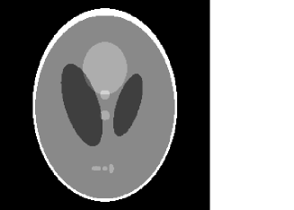
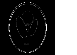
We demonstrate this point with the widely used Shepp-Logan phantom in Fig. 1. If the pixel values are labeled by $f_{s,t}$, the image gradient magnitude is:

$$|\vec{\nabla}f_{s,t}|=\sqrt{(f_{s,t}-f_{s-1,t})^{2}+(f_{s,t}-f_{s,t-1})^{2}}.$$ (1)

We refer to this quantity as the gradient image. The number of non-zero pixels in this 256x256 image is 32,668 , while the number of non-zero pixels in its gradient image is only 2,183.

To develop an iterative algorithm that takes advantage of this sparseness, the objective function to be minimized is the $\ell_{1}$-norm of the gradient image, otherwise known as the total variation (TV) of the image:

$$||f_{s,t}||_{TV}=\sum_{s,t}|\vec{\nabla}f_{s,t}|=\sum_{s,t}\sqrt{(f_{s,t}-f_{s-1,t})^{2}+(f_{s,t}-f_{s,t-1})^{2}}.$$ (2)

TV has been utilized in image processing for denoising of images while preserving edges Rudin et al. (1992); Vogel and Oman (1996), and TV has been suggested as a regularization function in Bayesian reconstruction, implemented in an EM algorithm Panin et al. (1999); Persson et al. (2001a, b). The use of the image TV here is different in that we seek an algorithm that is an implementation of an optimization program, which yields possibly the exact image for sparse data problems under the condition of exact data consistency.

Recently, a TV-based algorithm for recovering an image from sparse samples of its Fourier transform (FT) was developed Candes et al. (2004); Candes and Tao (2004). In that work the authors investigated the optimization program of minimizing the image TV under the constraint that the FT of the image matches the known FT samples. They showed that this optimization program satisfies an “exact reconstruction principle” (ERP) for sparse data: if the number of FT samples is twice the number of non-zero pixels in the gradient image, then this optimization program can yield a unique solution, which is in fact the true image for almost every image function. The algorithm for FT inversion from sparse samples was applied to image reconstruction from 2D parallel-beam data at few-views. The use of the FT-domain TV algorithm (FT-TV) to address the 2D parallel-beam problem was possible because of the central slice theorem, which links the problem to FT inversion.

The FT-TV algorithm, however, cannot be applied to image reconstruction for divergent-beam CT, i.e. fan-beam and cone-beam CT, because there is no central slice theorem to bring the projection data into the image’s Fourier space. The ERP of the FT-TV algorithm may extend to inversion of other linear systems from sparse data Candes and Tao (2004). To our knowledge, no TV-based algorithm that exploits the ERP and that is specific to tomographic image reconstruction from divergent-beam projections has been developed previously.

In this work, we investigate and develop a TV algorithm for image reconstruction from divergent-beam projections applicable to both fan-beam and cone-beam CT imaging. We present a TV iterative algorithm that can reconstruct accurate images from sparse or insufficient data problems that may occur due to practical issues of CT scanning. The sparse data problem that we consider here is reconstruction from few-view projections; whereas the insufficient data problems that we investigate are reconstructions from data acquired over a limited angular range or with a detector containing gaps due to bad detector bins. Much research has been done on image reconstruction algorithms for the few-view problem, see e.g. Refs. Li et al. (2002); Wu et al. (2003); Kolehmainen et al. (2003), and for the limited angular range problem, see e.g. Refs. Persson et al. (2001b); Delaney and Bresler (1998); Rantala et al. (2006). Comparison with these algorithms is a topic for future work, but we do present comparisons with the basic EM and ART algorithms. We point out that the comparison with EM and ART are only meant to reveal the ill-posedness of the imaging problems considered here. In Sec. II, we describe our TV iterative algorithm for tomographic image reconstruction from divergent-beam projection data. In Sec. III, we demonstrate and validate the proposed TV algorithm for image reconstruction in various sparse or insufficient data problems. In Sec. IV, we re-examine some of the examples of Sec. III under non-ideal conditions such as data inconsistency due to noise. Although the numerical results involve only fan-beam CT, the same algorithm can readily be applied to image reconstruction in cone-beam CT.

II Method

In this section, we describe our TV algorithm for image reconstruction in divergent-beam CT. The image function is represented in its discrete form as a vector $\vec{f}$ of length $N_{\text{image}}$ with individual elements $f_{j}$, $j=1,2,\dots,N_{\text{image}}$. When it is necessary to refer to pixels in the context of a 2D image we use the double subscript form $f_{s,t}$, where

$$j=(s-1)W+t;\;\;\;\;\;s=1,2,\dots,H;\;\;\;\;t=1,2,\dots,W;$$ (3)

and integers $W$ and $H$ are, respectively, the width and height of the 2D image array, which has a total number of pixels $N_{\text{image}}=W\times H$. The projection-data vector $\vec{g}$ has length $N_{\text{data}}$ with individual measurements referred to as $g_{i}$, $i=1,2,\dots,N_{\text{data}}$.

The general theoretical setting for the TV algorithm discussed here involves inversion of a discrete-to-discrete linear transform,

$$\vec{g}={\cal M}\vec{f},$$ (4)

where the system matrix ${\cal M}$ is composed of $N_{\text{data}}$ row vectors $\vec{M}_{i}$ that yield each data point, $g_{i}=\vec{M}_{i}\cdot\vec{f}$. The individual elements of the system matrix are $M_{ij}$. We seek to obtain an image represented by the finite vector $\vec{f}$ from knowledge of the data vector $\vec{g}$ and the system matrix ${\cal M}$. Mathematically, the problems we consider here involve insufficient data; namely the number of data samples $N_{\text{data}}$ is not enough to uniquely determine the $N_{\text{image}}$ values of the image vector $\vec{f}$ by directly inverting Eq. (4). The overall strategy is to incorporate the assumption of gradient image sparseness on the image function $\vec{f}$ to arrive at a solution from knowledge of the data $\vec{g}$.

To solve the linear system represented in Eq. (4) we develop a TV algorithm that implements the following optimization program Candes et al. (2005): Find $\vec{f}$ that

$$\min\|\vec{f}\|_{TV}\;\;\;\text{such that}\;\;\;{\cal M}\vec{f}=\vec{g},\;\;\;f_{j}\geq 0.$$ (5)

In the algorithm, the minimization of the image TV is performed by the gradient descent method, and the constraints imposed by the known projection data are incorporated by projection on convex sets (POCS) (see e.g. Sec. 15.4.5 of Ref. Barrett and Myers (2004)). We use POCS for enforcing the projection data constraint, because, even in the case of sparse sampling, the size of the projection data sets can be large, and POCS can efficiently handle large data sets. In the following we define the system matrix used for modeling the divergent-beam projections, and describe the TV algorithm for implementing the program in Eq. (5). We conjecture that the linear system matrices corresponding to the various scanning configurations studied in Secs. III and IV, below, support an ERP for insufficient data, and we demonstrate this possibility with numerical examples.

II.1 System matrix for the divergent-beam configuration

Figure 2: Fan-beam CT configuration used in the simulations presented in this work. The 256x256 image array is 20x20 cm², and the detector is composed of 512 bins. The center of rotation for the source-detector gantry coincides with the center of the image array.

In divergent-beam CT, the x-ray source is a single spot for each projection view. The projection data are captured on a 1D or 2D detector array for the fan-beam or cone-beam system. For illustration and introduction of the configuration used in the Secs. III and IV, we focus on the fan-beam configuration shown in Fig. 2. The detector is modeled as a straight-line array of 512 detector bins, which is large enough so that the field-of-view is the circle inscribed in the 256x256 imaging array. The CT measurements can be related to the path integral of the x-ray attenuation coefficient along the rays defined by the source spot and individual detector bins. In the discrete setting, these ray integrals can be written as weighted sums over the pixels traversed by the source-bin ray as

$$d_{i}=\sum_{j=1}^{N_{\text{image}}}M_{ij}f_{j},\;\;\;\;\;\text{where}\;\;\;\;\;i=1,2,\dots,N_{\text{data}}.$$ (6)

To model the fan-beam projection of the discrete image array, we employ the ray-driven projection model where the system matrix weights $M_{ij}$ are computed by calculating the intersection length of the $i$th ray through the $j$th pixel. The ray-driven system matrix is illustrated for a 5x5 image array in Fig. 3. There are other ways to model the discrete projection such as pixel-driven and distance-driven models De Man and Basu (2004), which provide alternative definitions of pixel weights. Even though the system matrix discussed here is for the fan-beam configuration, extension to cone-beam 3D imaging is straight-forward.

Figure 3: The ray passing through this 5x5 image array illustrates an individual row vector of the system matrix $\vec{M}_{i}$. In this case the data point $d_{i}$ is calculated as $d_{i}=\sum_{j=1}^{25}M_{ij}f_{j}$, where $M_{ij}$ is the length of the $i$th ray traversing the $j$th pixel. The illustrated system matrix has non-zero entries only on image pixels $f_{1}$, $f_{6}$, $f_{7}$, $f_{8}$, $f_{9}$, $f_{14}$, and $f_{15}$ .

An interesting difference, between the TV algorithm presented here and the FT-TV algorithm of Ref. Candes et al. (2004), is the construction of the system matrix. In Ref. Candes et al. (2004), the 2D parallel-beam data are processed by taking a 1D FT along the detector coordinate, and the system matrix is the discrete 2D FT. In this work the system matrix represents directly the discrete ray integration of the image, and there is no transformation of the projection data. Thus, even in the limit that the focal length of the fan-beam tends to infinity, our TV algorithm does not yield the FT-TV algorithm.

II.2 Computation of TV gradient and realization of data constraint

The TV algorithm minimizes the TV of the image estimate, which can be accomplished by use of the gradient descent method Candes et al. (2004) and other optimization methods. Performing the gradient descent requires the expression for the gradient of the image TV. This gradient can also be thought of as an image, where each pixel value is the partial derivative of the image TV with respect to that pixel. Taking the derivative of $\left\|\vec{f}\right\|_{TV}$ with respect to each pixel value results in a singular expression. We thus use the following approximate derivative,

$$v_{s,t}=\frac{\partial\left\|\vec{f}\right\|_{TV}}{\partial f_{s,t}}\approx\frac{2\left(f_{s,t}-f_{s-1,t}\right)+2\left(f_{s,t}-f_{s,t-1}\right)}{\sqrt{\epsilon+\left(f_{s,t}-f_{s-1,t}\right)^{2}+\left(f_{s,t}-f_{s,t-1}\right)^{2}}}\\ -\frac{2\left(f_{s+1,t}-f_{s,t}\right)}{\sqrt{\epsilon+\left(f_{s+1,t}-f_{s,t}\right)^{2}+\left(f_{s+1,t}-f_{s+1,t-1}\right)^{2}}}\\ -\frac{2\left(f_{s,t+1}-f_{s,t}\right)}{\sqrt{\epsilon+\left(f_{s,t+1}-f_{s,t}\right)^{2}+\left(f_{s,t+1}-f_{s-1,t+1}\right)^{2}}},$$ (7)

where $\epsilon$ is a small positive number; for the results below we used $\epsilon=10^{-8}$. Note that this expression is valid for non-border pixels. We refer to the resulting gradient vector as $\vec{v}$, and just as with the image vector, its individual elements can be denoted by either a single index $v_{j}$ or pixel indexes $v_{s,t}$. In the actual algorithm, we employ the normalized TV gradient $\hat{v}$.

We use the POCS method to realize the linear system constraints in Eq. (5). Each measured point $g_{i}$ of the data vector specifies a hyperplane in the $N_{\text{image}}$-dimensional space of all possible solutions $\vec{f}$. The basic POCS method projects the current estimate of $\vec{f}$ onto the hyperplanes, which are convex sets, corresponding to each data point in sequential order. By repeating this process the image estimate moves toward the intersection of all of these hyperplanes, which is the sub-space of valid solutions to the linear system. In our POCS implementation, we will also include the positivity constraint.

II.3 TV algorithm for divergent-beam CT

Having specified the system matrix, TV gradient, and data constraints, we now describe the iterative steps of the TV algorithm, which implements the optimization program described in Eq. (5) for image reconstruction from divergent-beam data. Each iteration consists of two phases: POCS and gradient descent. The POCS phase is further broken down into two steps that enforce data consistency and positivity. As a result, the steps comprising each loop are: the DATA-step, which enforces consistency with the projection data; the POS-step, which ensures a non-negative image; and the GRAD-step, which reduces the TV of the image estimate. The iteration performed in the algorithm has two levels: the overall iteration number is labeled by $n$, and the sub-iterations in the DATA- and GRAD-steps are labeled by $m$. The image vector during the iterations of the DATA-step is $\vec{f}^{(TV-DATA)}[n,m]$, indicating the $m$th DATA-step sub-iteration within the $n$th iteration. We use $\vec{f}^{(TV-POS)}[n]$ to denote the image estimate after projection onto the non-negative half-plane. Finally, $\vec{f}^{(TV-GRAD)}[n,m]$ represents the $m$th gradient descent step within the $n$th iteration. The steps of the algorithm are:
(A) Initialization:

$$n=1\;\;\;\text{and}\;\;\;\vec{f}^{(TV-DATA)}[n,1]=0;$$ (8)

(B) Data projection iteration, for $m=2,\dots,N_{\text{data}}$:

$$\vec{f}^{(TV-DATA)}[n,m]=\vec{f}^{(TV-DATA)}[n,m-1]-\vec{M}_{m-1}\frac{g_{m-1}-\vec{M}_{m-1}\cdot\vec{f}^{(TV-DATA)}[n,m-1]}{\vec{M}_{m-1}\cdot\vec{M}_{m-1}};$$ (9)

(C) Positivity constraint:

$$(f_{j})^{(TV-POS)}[n]=\begin{cases}(f_{j})^{(TV-DATA)}[n,N_{\text{data}}]&(f_{j})^{(TV-DATA)}[n,N_{\text{data}}]\geq 0\\ 0&(f_{j})^{(TV-DATA)}[n,N_{\text{data}}]<0\end{cases};$$ (10)

(D) TV gradient descent initialization:

$$\vec{f}^{(TV-GRAD)}[n,1]=\vec{f}^{(TV-POS)}[n];$$

$$d_{A}(n)=\left\|\vec{f}^{(TV-DATA)}[n,1]-\vec{f}^{(TV-POS)}[n]\right\|_{2};$$ (11)

(D^′) TV gradient descent, for $m=2,\dots,N_{\text{grad}}$:

$$\vec{v}_{s,t}[n,m-1]=\left.\frac{\partial\|\vec{f}\|_{TV}}{\partial f_{s,t}}\right|_{f_{s,t}=f^{(TV-GRAD)}_{s,t}[n,m-1]};\;\;\;\;\;\hat{v}[n,m-1]=\frac{\vec{v}[n,m-1]}{\left|\vec{v}[n,m-1]\right|};$$

$$\vec{f}^{(TV-GRAD)}[n,m]=\vec{f}^{(TV-GRAD)}[n,m-1]-a{d_{A}(n)}\hat{v}[n,m-1];$$ (12)

(E) Initialize next loop:

$$\vec{f}^{(TV-DATA)}[n+1,1]=\vec{f}^{(TV-GRAD)}[n,N_{\text{grad}}];$$ (13)

Increment $n$ and return to step (B). In the text, when we refer to the iteration number of the TV algorithm, we mean the iteration number of the outer loop indicated by the index $n$. The iteration is stopped when there is no appreciable change in the intermediate images after the POCS steps; namely the difference between $\vec{f}^{(TV-POS)}[n]$ and $\vec{f}^{(TV-POS)}[n-1]$ is “small”.

The distance $d_{A}(n)$ provides a measure for the difference between the image estimate before the DATA-step and the estimate after the enforcement of positivity. The gradient descent procedure is controlled by specifying the parameter $a$, the fraction of the distance $d_{A}(n)$ along which the image is incremented, and $N_{grad}$ the total number of gradient descent steps that are performed. The algorithm relies on the balance between the POCS phase (DATA- and POS-steps) and the gradient descent. By scaling the size of the gradient descent step with $d_{A}(n)$, the relative importance of the POCS and gradient descent stages of the algorithm maintains this balance. As long as the total change in the image due to the gradient descent does not exceed the change in the image due to POCS the overall iteration steps will steer the image estimates closer to the solution space of the imaging linear system.

If the step size of the gradient descent is too strong the image becomes uniform and inconsistent with the projection data. On the other hand, if the step size of the gradient descent is too small, the algorithm reduces to standard ART with a positivity constraint included. For the results shown in this article we selected $a=0.2$, and $N_{grad}=20$. These values strikes a good balance between the POCS steps and the TV-gradient descent, and they seem to work well for a wide range of reconstruction problems, including those addressed in Secs. III and IV below. The algorithm appears to be robust in that changes to the parameters only appear to alter the convergence rate and not the final image. Further investigation of the algorithm parameters may improve the convergence speed.

III Numerical Results: ideal conditions

For the results in this section, we demonstrate and validate our TV algorithm under “ideal” conditions. The true image solution is taken to be the Shepp-Logan image shown in Fig. 1 discretized on a 256x256 pixel grid. This phantom is often used in evaluating tomographic reconstruction algorithms. As also shown in Fig. 1, its gradient image is sparse with only 2,183 non-zero pixels. This number is roughly only 6.7% of the 32,668 non-zero pixels of the Shepp-Logan image itself. Taking the result for Fourier inversion Candes et al. (2004) as a rule of thumb for the current problem, one might expect that a minimum of twice as many non-zero, independent projection measurements are needed for obtaining the image. Thus we suppose that a minimum of 4,366 measurements are required for the ERP. We first demonstrate the image recovery from sparse data with the few-view example shown below. Subsequently, we show the utility of the TV algorithm for other insufficient data problems where there are plenty of projection ray measurements, but the angular or projection coverage is less than the minimum for analytic reconstruction. The insufficient data problems demonstrated below are the limited scanning angle problem, and the “bad bins” problem where there is a gap on the detector for all available projection views.

For the numerical experiments presented here, the simulated fan-beam configuration are variations on the configuration shown in Fig. 2. In the first set of experiments the data used are ideal in the sense that they are the exact line integrals, up to round-off error in the computer, of the discrete 256x256 Shepp-Logan image. The data are, however, severely under-determined so that there would be no chance of directly solving the linear equation, in Eq. (4). The detector modeled has 512 bins, and the total number of measured rays is 512 multiplied by the number of view angles. But the important number is actually the total number of non-zero measurements, and this is stated with each example discussed below.

In order to illustrate the degree of ill-posedness for each numerical example, we compare the proposed TV algorithm with standard EM and ART algorithms, which have been widely applied to solving the under-determined or unstable linear systems in tomographic imaging. A unique feature of EM is that the positivity constraint is built-in to the algorithm, and for CT imaging applications the object function is positive. The EM implementation used here is basic, specified by the following update equation:

$$f_{j}^{\text{(EM)}}[n]=f_{j}^{\text{(EM)}}[n-1]\frac{\sum_{i}{\left(M^{T}\right)_{ji}}\frac{g_{i}}{\sum_{j}{M_{ij}}f_{j}^{\text{(EM)}}[n-1]}}{\sum_{i}{\left(M^{T}\right)_{ji}}}.$$ (14)

In our studies, we used no regularization during the iterations.

The ART algorithm is identical to the TV algorithm discussed in Sec. II.3 except that step (D), the minimization of the image TV, is not performed. The steps for the ART algorithm are:
(A) Initialization

$$n=1;\;\;\;\;\;\vec{f}^{(ART-DATA)}[n,1]=0;$$ (15)

(B) Data-projection iteration, for $m=2,\dots,N_{\text{data}}$:

$$\vec{f}^{(ART-DATA)}[n,m]=\vec{f}^{(ART-DATA)}[n,m-1]-\vec{M}_{i}\frac{g_{i}-\vec{M}_{i}\cdot\vec{f}^{(ART-DATA)}[n,m-1]}{\vec{M}_{i}\cdot\vec{M}_{i}};$$ (16)

(C) Positivity constraint:

$$(f_{j})^{(ART-POS)}[n]=\begin{cases}(f_{j})^{(ART-DATA)}[n,N_{\text{data}}]&(f_{j})^{(ART-DATA)}[n,N_{\text{data}}]\geq 0\\ 0&(f_{j})^{(ART-DATA)}[n,N_{\text{data}}]<0\end{cases};$$ (17)

(D) Initialization next loop:

$$\vec{f}^{(ART-DATA)}[n+1,1]=\vec{f}^{(ART-POS)}[n];$$ (18)

Increment $n$ and return to step (B). Again, no explicit regularization was performed during the ART iterations. For both EM and ART algorithms the iteration was stopped when there was no appreciable change in the image.

No explicit regularization for the EM and ART algorithms was used for two reasons. First, we wish to demonstrate only the degree of ill-posedness of the linear systems corresponding to the various scanning configurations investigated below. And this is effectively demonstrated by using well-known algorithms such as EM and ART. Second, we are comparing the TV algorithm with the EM and ART algorithms on how well they solve the linear system corresponding to sparse sampling or insufficient projection data. The data used for the bulk of the examples are ideal (up to machine precision), and any explicit regularization during the EM or ART iterations would introduce inconsistency between the reconstructed image and the projection data.

III.1 Few-view results

The first case is a reconstruction problem from few-view projections in fan-beam CT. Using the Shepp-Logan phantom shown in Fig. 4A, we generated projection data at 20 view angles specified by:

$$\theta_{i}=\begin{cases}18^{\circ}*(i-1)&1\leq i\leq 10\\ 18^{\circ}*(i-0.5)&10<i\leq 20.\end{cases}$$ (19)

Though sparse, the angles cover 360^∘ about the object. The shift in the second half of the angular measurements helps to reduce redundancy in the scanned data. The total number of measurement rays is $512\times 20=10,240$, but only 8,236 of these projection elements are non-zero. This number is larger than the twice the support of the gradient image, but it is well below the support of the Shepp-Logan phantom itself. In addition, the angular direction is severely undersampled.

Figure 4: Upper row: The true image and images reconstructed by use of the TV, EM, and ART algorithms from 20-view projection data. The display gray scale is [0.85,1.15]. Middle row: Image profiles along the centers of the images in the horizontal and vertical directions obtained with the TV algorithm (thick line). Lower row: Image profiles along the centers of the images in the horizontal and vertical directions obtained with the EM (dashed lines) and ART (dotted lines) algorithms. The corresponding true profiles are plotted as the thin lines in the middle and lower rows.

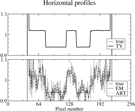
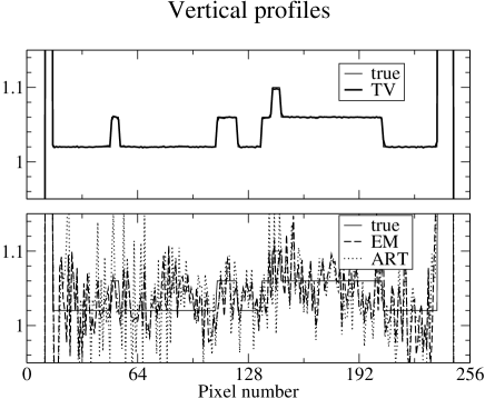
From the projection data generated at the 20 views, we reconstructed images, as shown in row one of Fig. 4, by use of the TV, EM, and ART algorithms. The number of iterations for each algorithm was 200. For a quantitative comparison, we also compare the image profiles along the central lines of the images in the horizontal and vertical directions. The results in Fig. 4 indicate that the TV reconstruction is visually indistinguishable from the true image, suggesting that the system matrix corresponding to sparse fan-beam data may have the ERP even though the column vectors of the system matrix do not form an ortho-normal basis. The EM and ART results show considerable artifacts.

Figure 5: Images for the random ellipses (upper row), the random spots (middle row), and lines (lower row) phantoms. The true and gradient images of these phantoms are displayed in columns one and two, respectively. Images reconstructed from 20-view projections by use of the TV algorithm are displayed in column three. The gray scales for the images are [0.95, 1.15] for row one and [0.9, 1.1] for rows two and three.

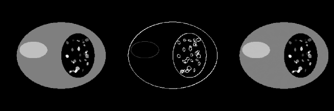
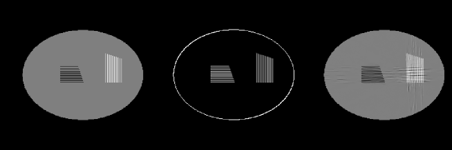
In an attempt to demonstrate the wide applicability of the TV algorithm, we have also applied it – without changing any parameters in the algorithm – to three additional phantoms, as shown in the first column of Fig. 5. The properties of these phantoms are as follows. The “random ellipse” phantom consists of 10 randomly selected ellipses on a uniform circular background with a value of 1.0. The values of each of the ellipses was randomly selected in the range of [1.01, 1.10]. The “random spots” phantom is similar in that 30 randomly selected small ellipses within the value range of [0.9, 1.1] are placed in an air cavity. The background ellipse has a value of 1.0 and and additional ellipse with a value of 1.05 is placed on the left of the phantom. The spots and the air gap are meant to resemble, roughly, the lung. The “lines” phantom consists of 2 groups of 10 lines at values of 0.9 and 1.1 on a background ellipse of value 1.0. As with the other phantoms, the gradient image of the lines phantom has sparse structures as shown in the second column of Fig. 5. But the lines phantom is designed in such a way as to provide a stiff challenge for the TV algorithm. It is known for the FT-inversion problem that certain regular structures in the image may be difficult to reconstruct by use of the FT-TV algorithm because of the small support of such images in Fourier space Candes et al. (2004). We expect that such images also pose a challenge for the TV algorithm developed in this work.

Using these phantoms, we generated fan-beam projection data at 20 views (uniformly distributed over $2\pi$, specified by Eq. (19)). We show in column three of Fig. 5 the TV reconstructions for the random ellipses (upper row), the random spots (middle row), and lines (lower row) phantoms. The reconstructions for the random ellipses and random spots phantoms are visually indistinguishable from their corresponding truth. As expected the lines phantom proves to be challenging. Although the reconstruction for the lines phantom does show some artifacts, it is still impressive. A quick glance at the EM and ART results in Fig. 4 will remind the reader how unstable image reconstruction is for this few-view scanning configuration.

III.2 Limited-angle problems

An important application of the TV algorithm may be for reconstruction problems where there are insufficient data in the corresponding continuous case. For example, the scanning angle may be less than 180^∘ plus the fan angle in fan-beam CT, or there may be gaps on the detector for each projection when the data are known to be bad for certain detector bins. For continuous functions of compact support it is well-known that data in a scanning range of 180^∘ plus the fan-angle is sufficient for stable image reconstruction in fan-beam CT. For the fan-beam configuration described above, 180^∘ plus the fan angle is 209^∘. For scanning angular ranges less than 209^∘, the corresponding discrete linear system is likely to be generally be ill-posed.

Figure 6: Upper row: The true image and images reconstructed by use of the TV, EM, and ART algorithms from data over 180^∘. The display gray scale is [0.85,1.15]. Middle row: Image profiles along the centers of the images in the horizontal and vertical directions obtained with the TV algorithm (thick line). Lower row: Image profiles along the centers of the images in the horizontal and vertical directions obtained with the EM (dashed lines) and ART (dotted lines) algorithms. The corresponding true profiles are plotted as the thin lines in the middle and lower rows.

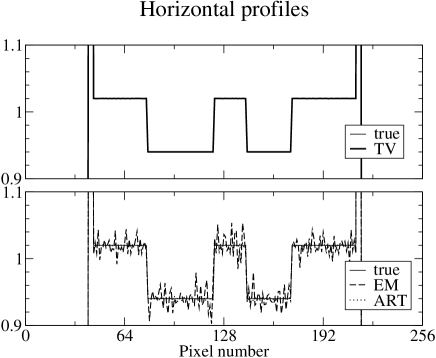
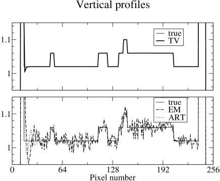
In the first limited-angle problem, we reduce the scanning angular range from 209^∘ to 180^∘ and generate projection data at 128 uniformly distributed views from the Shepp-Logan phantom. Again, the detector at each view has 512 bins. For this scan, the number of non-zero data points is 52,730 , which is even more than the number of non-zero pixels in the Shepp-Logan phantom itself.

We display in the upper row of Fig. 6 images reconstructed from this set of data by use of the TV, EM, and ART algorithms. The profiles of these images along the central horizontal and vertical rows are displayed in the middle and lower rows. The number of iterations for each of the TV, EM, and ART reconstructions is 1000. The images in row one of Fig. 6 show that the TV reconstruction is virtually indistinguishable from the true phantom and that the images obtained by use of the EM and ART algorithms are also reasonably accurate with only small distortion near the bottom of the images. This distortion of the EM and ART images is understandable because the 180^∘ scan covered the top half of the phantom. The high iteration numbers were used for achieving convergence in the bottom half of the image. Additionally, the EM image shows a high frequency artifact not seen in the TV or ART images, because the back-projector in each case is ray-driven, which is known to yield such Moire patterns in EM images De Man and Basu (2004). But, as explained above, we are comparing the reconstruction algorithms on their ability to solve the linear system corresponding to the imaging model, and we therefore use the ray-driven backprojection because it represents exactly the system-matrix adjoint.

Figure 7: Upper row: The true image and images reconstructed by use of the TV, EM, and ART algorithms from data over 90^∘. The display gray scale is [0.85,1.15]. Middle row: Image profiles along the centers of the images in the horizontal and vertical directions obtained with the TV algorithm (thick line). Lower row: Image profiles along the centers of the images in the horizontal and vertical directions obtained with the EM (dashed lines) and ART (dotted lines) algorithms. The corresponding true profiles are plotted as the thin lines in the middle and lower rows.

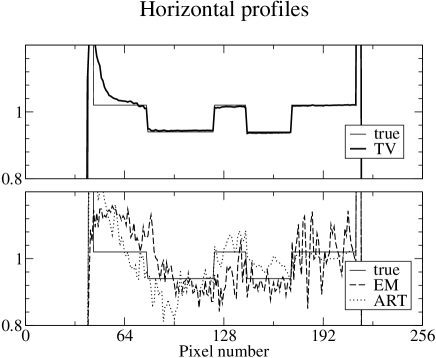
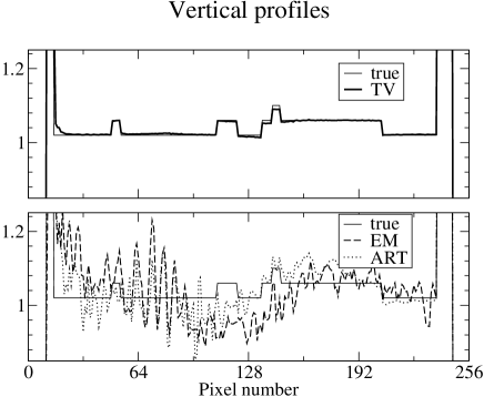
We explore further reduction in the scanning angle by taking 64 angular samples uniformly distributed over an angular range of only 90^∘, covering the first quadrant of the Shepp-Logan phantom in Fig. 7. We display in row one of Fig. 7 images reconstructed by use of the TV, EM, and ART algorithms. The number of iterations for the TV, EM, and ART reconstructions is 10,000. In this case, there were 26,420 non-zero projection measurements, which would seem to be sufficient for the TV algorithm considering the sparseness of the phantom’s image gradient. But the instability of the corresponding linear system appears to be too strong for accurate image reconstruction as can be seen in the reconstructions shown in the upper row of Fig. 7. In the middle row of Fig. 7, we show the profiles along central lines in the horizontal and vertical directions of the TV image. The corresponding true profiles are also displayed as the thin lines. The TV image contains a deviation from the true phantom on the left-hand edge, which is evident in the shown horizontal profile. On the other hand, the EM and ART reconstructions are highly distorted. We have studied in row three of Fig. 7 the profiles along central lines in the horizontal and vertical directions of the EM and ART images. Distortions in these images are clearly shown in these profile plots. We have also studied the image error as a function of iteration number in an effort to determine whether or not the TV algorithm will converge to the true image. For the previous cases the image error was tending to zero, but for this 90^∘ scan the image error appears to converge to a small but finite positive number. The system matrix corresponding to the 90^∘ scan appears to violate somewhat the ERP.

III.3 Projection data with “bad” detector bins

Another reconstruction problem of practical interest is how to handle the situation where data from a set of bins on the detector are corrupted. Such a problem could occur if there is a hardware failure or if the photon count is very low so that signal noise dominates. For fan-beam CT, if a full scan is performed over 360^∘, one may fill the gaps in the detector bins by using redundant data at conjugate views. For a short-scan, however, this approach may not be possible. Specifically, consider projection data displayed in Fig. 8; the angular range scanned is the minimum for exact reconstruction, namely, 180^∘ plus the fan angle, which in this case is a total of $209^{\circ}$. The projection data at each view, however, has a gap. Because the scanning angle is over the minimum range, there may not be redundant information to fill in the gap left by the “bad” detector bins. Direct application of analytic algorithms such as fan-beam FBP will yield conspicuous artifacts, as the implicit assumption is that the missing values are zero, which is highly inconsistent with the rest of the data function.

Figure 8: Intensity plot of the “bad bins” projection data function. The angular range covers 209^∘, which is the short-scan angle for the current fan-beam configuration. However, data at 30 of the 512 detector bins are missing.

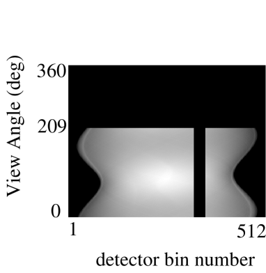
We apply the TV algorithm to reconstructing images from data shown in Fig. 8, which are generated at 150 views uniformly distributed over 209^∘. The detector at each view contains 512 bins, of which the data of 30 bins have been discarded as shown in Fig. 8. Again, in this case there may be enough data to determine the image, because the number of non-zero projection measurements is 58,430. The question is whether or not the corresponding linear system is stable enough that the solution can be found.

Figure 9: Upper row: The true image and images reconstructed by use of the TV, EM, and ART algorithms from data containing bad detector bins. The display gray scale is [0.85,1.15]. Middle row: Image profiles along the centers of the images in the horizontal and vertical directions obtained with the TV algorithm (thick line). Lower row: Image profiles along the centers of the images in the horizontal and vertical directions obtained with the EM (dashed lines) and ART (dotted lines) algorithms. The corresponding true profiles are plotted as the thin lines in the middle and lower rows.

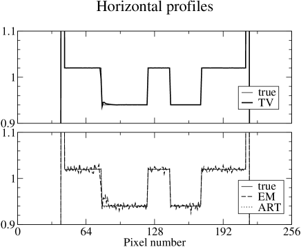
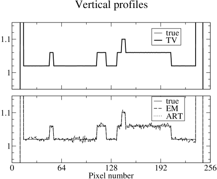
We display in Fig. 9 images reconstructed by use of the TV, EM, and ART algorithms. Once again, the TV image is visually indistinguishable from the true image, and both EM and ART algorithms yield in this case quite accurate images. In this study, the TV algorithm appears to be more robust than the EM and ART algorithms, because the TV image is obtained with only a 100 iterations while both the EM and ART algorithms required 10000 iterations to achieve the image accuracy shown in Fig. 9. We note that the previous FT-TV algorithm cannot address the bad bins problem directly even in the parallel-beam case, because it is not possible to perform the FT of the detector data at each view when there is a gap.

III.4 Few-view projection data with bad bins

The previously discussed insufficient data problems can be combined. For example, we consider the few-view problem discussed in Sec. III.1 with each projection view containing bad bins, as in the previous section. For this experiment we take projections at 20 views uniformly covering the short-scan angular range with the same detector gap as shown in Fig. 8. Thus the difference between this study and the one of Sec. III.3 is that the angular spacing between projections here is roughly 10^∘ instead of the 1.4^∘ spacing in the previous section. The few-view-projection data are sparse, and only 7735 measured data points are non-zero.

Figure 10: Upper row: The true image and images reconstructed by use of the TV, EM, and ART algorithms from 20-view data containing bad detector bins. The display gray scale is [0.85,1.15]. Middle row: Image profiles along the centers of the images in the horizontal and vertical directions obtained with the TV algorithm (thick line). Lower row: Image profiles along the centers of the images in the horizontal and vertical directions obtained with the EM (dashed lines) and ART (dotted lines) algorithms. The corresponding true profiles are plotted as the thin lines in the middle and lower rows.

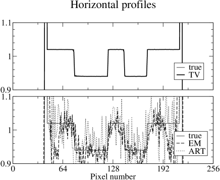
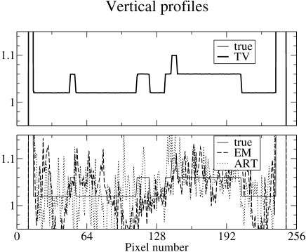
We show in Fig. 10 images reconstructed by use of the TV, EM, and ART algorithms. The TV image is once again visually indistinguishable from the true phantom. Thus, it appears that the system matrix corresponding to this scanning configuration fulfills the ERP. The EM and ART reconstructions show similar artifacts as were seen in the few-view results shown in Sec. III.1. In addition, there appears to be additional artifacts from the missing detector bins.

The proposed TV algorithm can address a host of other sparse data problems. The key points for the success of the algorithm – under ideal conditions described above – are that the support of the data function be at least twice the support of the gradient of the true image and that the corresponding linear system is not too ill-conditioned as was seen for the 90^∘-scan case.

IV Numerical Results: complicating factors

The results of the previous section assumed the ideal situation of perfect consistency among the measured projection rays and a sufficiently sparse gradient image. We show below how the TV, EM, and ART algorithms compare when these conditions are not strictly held, by adding a varying background, to violate gradient sparseness, or by adding signal noise, to violate data consistency.

IV.1 Violation of gradient sparseness

In many applications the gradient images may be sparse only in an approximate sense. Even though it is a good approximation to assume that images will be constant over many regions, there will also be situations in which the images will have some level of variation within the regions. An important question is whether or not a low amplitude violation of gradient sparseness leads to only small deviations in images reconstructed by use of the TV algorithm. We investigate this issue by repeating the few-view and bad-bin studies described in Secs. III.1 and III.3, but adding a wavy background to the Shepp-Logan phantom.

Figure 11: Upper row: The true image with a wavy background and images reconstructed by use of the TV, EM, and ART algorithms from 20-view data. The display gray scale is [0.85,1.15]. Middle row: Image profiles along the centers of the images in the horizontal and vertical directions obtained with the TV algorithm (thick line). Lower row: Image profiles along the centers of the images in the horizontal and vertical directions obtained with the EM (dashed lines) and ART (dotted lines) algorithms. The corresponding true profiles are plotted as the thin lines in the middle and lower rows.

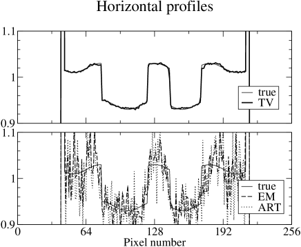
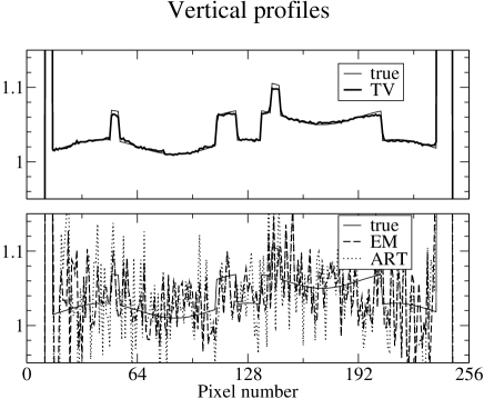
Using the Shepp-Logan phantom with a wavy background in Fig. 11, we generated projection data at 20 views specified by Eq. (19). The amplitude of the wavy background is 1% of the gray matter attenuation coefficient. Any negative values in the phantom are thresholded to zero, so as to allow the applicability of the EM algorithm. With the wavy background the number of non-zero pixels in the gradient image jumps to 51,958 , but the majority of these non-zero values are small compared to the gradients at the boundaries of the different tissues. As was the case with the previous few-view study, the number of measurements is 10,240, which is less than twice the number of non-zero pixels in the gradient image, violating the sparseness condition.

In Fig. 11, we show the images reconstructed by use of the TV, EM, and ART algorithms from the 20-view data. The iteration numbers for obtaining these results were 200, 1000, and 500 for the TV, EM, and ART algorithms, respectively. The images in Fig. 11 indicate that the TV reconstruction is visually almost indistinguishable from the true image and that the EM and ART algorithms have difficulty with this data set. Upon further inspection of the image profiles, it can be seen that the TV algorithm does not yield an exact reconstruction. The small violation, however, of the gradient image sparseness does not appear to lead to large errors in the reconstructed image. We point out once again that this example does not constitute a mathematical proof, but it is suggestive of the conclusion that small violations in the gradient sparseness yields only small errors in the reconstructed image.

Figure 12: Upper row: The true image with a wavy background and images reconstructed by use of the TV, EM, and ART algorithms from bad detector bin data. The display gray scale is [0.85,1.15]. Middle row: Image profiles along the centers of the images in the horizontal and vertical directions obtained with the TV algorithm (thick line). Lower row: Image profiles along the centers of the images in the horizontal and vertical directions obtained with the EM (dashed lines) and ART (dotted lines) algorithms. The corresponding true profiles are plotted as the thin lines in the middle and lower rows.

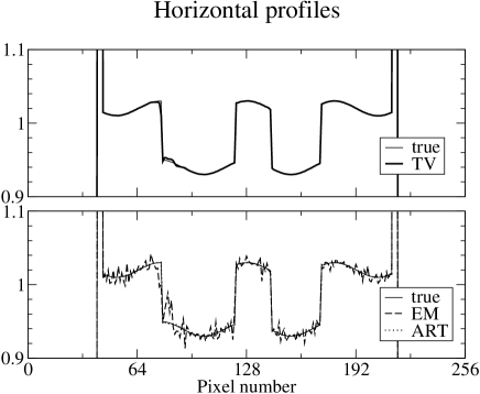
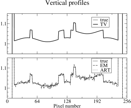
We also reexamined image reconstruction from data containing bad-bins of Sec. III.3 with the $1\%$ low amplitude wavy background added to the original image. In this case, the number of projection data is 58,430, which is not twice the number of non-zero pixels in the image but it is a comparable number. We display in Fig. 12 images reconstructed by use of the TV, EM, and ART algorithms. It can be observed that the TV image is visually indistinguishable from the true image. We also note that, as before, the ART and EM reconstructions are close to the original image in this case. The number of iterations for the TV algorithm is 100, which is much less than the 10,000 iterations used for both EM and ART algorithms.

IV.2 Reconstruction from noisy data

Another omni-present physical factor that contributes to data inconsistency is signal noise in the projection measurements. It is of practical significance to evaluate the performance of the TV algorithm in the presence of data noise. While a thorough evaluation of the noise properties of the TV algorithm is beyond the scope of this work, we present preliminary results indicating that the TV algorithm appears to be effective on sparse data problems even when the data contain inconsistencies due to signal noise. For the noise studies, we again take the few-view and bad-bin cases in Secs. III.1 and III.3. In each case, Gaussian noise is introduced in the projection data at the level of 0.1$\%$ of the ideal measurement values.

The total variation algorithm has an interesting and practical feature with respect to data sets that contain inconsistencies. Even though TV minimization is part of a larger algorithm that implements the program in Eq. (5), the gradient descent phase happens to also regularize the image. This feature of the TV algorithm is particularly useful in the present case of data inconsistencies. As a result, for this section we present two images from the TV algorithm: $f^{(TV-GRAD)}[n,N_{\text{grad}}]$, the image after the completion of the gradient descent phase, and $f^{(TV-POS)}[n]$, the image after the completion of the POCS phase. The former image is labeled TV1 and the latter TV2. The TV1 image is seen to be a regularized version of the TV2 image.

Figure 13: Images reconstructed from 20-view noisy data by use of the TV algorithm after the gradient descent phase (TV1) and after the projection phase (TV2) and by use of the EM and ART algorithms.

For the few-view study, we show in Fig. 13 images reconstructed by use of the TV (labeled TV1 and TV2), EM, and ART algorithms. The iteration numbers for the TV, EM and ART images are 200, 200, and 100, respectively. In the studies with consistent data above, the differences between the TV1 and TV2 images were numerically negligible. With inconsistencies resulting from data noise, however, there is a marked difference. The image $f^{(TV-GRAD)}[n,N_{\text{grad}}]$ after the gradient descent phase is clearly a regularized version of the image $f^{(TV-POS)}[n]$ obtained after the data projection and positivity constraint. Depending on the task, either image may prove useful for a particular imaging application. For the few-view study, both images $f^{(TV-GRAD)}[n,N_{\text{grad}}]$ and $f^{(TV-POS)}[n]$ obtained with the TV algorithm appear to have less artifacts than the EM and ART reconstructions in Fig. 13. We point out again that no explicit regularization is performed with EM or ART in the studies here and below aside from the fact that we truncate the iteration numbers at 200 and 100 in the EM and ART algorithms, respectively.

Figure 14: Images reconstructed from bad-bin noisy data by use of the TV algorithm after the gradient descent phase (TV1) and after the projection phase (TV2) and by use of the EM and ART algorithms.

For the bad bin case, we generated noisy data by adding Gaussian noise, at the level of 0.1% of the individual true data values, to the noiseless data described in Sec. III.3. In Fig. 14, we show images reconstructed by use of the TV algorithm (TV1) and (TV2), the EM, and the ART algorithm. The iteration numbers for the TV, EM, and ART images are 200, 200, and 100, respectively. Again, we show two TV images in Fig. 13: TV1 and TV2. The results of this study suggests that the TV and EM algorithms can still effectively correct for the effect of the missing detector bins. The ART algorithm, which showed very mild streaking in Fig. 9 under the ideal condition, displays significant streaking due to the combination of signal noise and bad detector bins.

V Discussion and Conclusion

In this article, we have developed a TV algorithm for accurate image reconstruction in divergent-beam CT under a number of imperfect sampling situations. We have evaluated and demonstrated the performance of the TV algorithm in addressing a number of challenging reconstruction problems, including the few-view, limited-angle, and bad-bin problems. As results in these numerical studies indicate, the proposed TV algorithm can yield accurate reconstructions in these difficult cases, which are of practical significance. The effectiveness of the TV algorithm relies on the fact that the object being imaged has a relatively sparse gradient image. It should be pointed out that we did not provide a theoretical proof of the ERP conjecture for the various scanning configurations studied here; however, we speculate based on the numerical examples that this principle may apply to many insufficient data problems in divergent-beam CT. In future work we will compare the TV algorithm with state-of-the-art implementations of EM and ART, and compare with algorithms that have been designed to handle few-view Li et al. (2002); Wu et al. (2003); Kolehmainen et al. (2003) and limited angular range Persson et al. (2001b); Delaney and Bresler (1998); Rantala et al. (2006) problems. The TV algorithm described above applies equally to cone-beam CT, even though our examples were limited to fan-beam CT. The TV algorithm may also prove useful for other tomographic imaging modalities.

There are numerous aspects of the TV algorithm that may make it relevant and useful for medical and industrial CT imaging. The assumption of a sparse gradient image is quite reasonable for many object functions in medical and industrial applications, because often sought-after quantities such as x-ray attenuation coefficient are relatively constant over extended areas or volumes. We showed example reconstructions from data containing two of the most likely imperfections. First, one can expect that the sparseness of the image gradient will hold only approximately, and second, there will always be some level of inconsistency among the projection data due to signal noise. Our numerical studies with respect to these complicating factors appear to show that the TV algorithm can effectively reconstruct quantitatively accurate images from imperfectly sampled data. We are currently investigating the application of the TV algorithm to 3D cone-beam CT where there are a host of imperfect sampling situations that have practical significance. We will also investigate and develop refinements to the TV algorithm that optimize its performance.