The Young Stellar Population of IC 1613

Abstract

Context. Determining the parameters of massive stars is crucial to understand many processes in galaxies and the Universe, since these objects are important sources of ionization, chemical enrichment and momentum. 10m class telescopes enable us to perform detailed quantitative spectroscopic analyses of massive stars in other galaxies, sampling areas of different metallicity. Relating the stars to their environment is crucial to understand the physical processes ruling their formation and evolution.

Aims. In preparation for the new instrumentation coming up on the GTC, our goal is to build a list of massive star candidates in the metal-poor irregular galaxy IC 1613. The catalogue must have very high astrometric accuracy, apt for the current generation of multi-object spectrographs. A census of OB associations in this galaxy is also needed, to provide important additional information about age and environment of the candidate OB stars.

Methods. From INT-WFC observations, we have built an astrometric and photometric catalogue of stars in IC 1613. Candidate blue massive stars are preselected from their colors. A friends-of-friends algorithm is developed to find their clustering in the galaxy. While a common physical origin for all the members of the associations cannot be ensured, this is a necessary first step to place candidate OB stars in a population context.

Results. We have produced a deep catalogue of targets in IC 1613 that covers a large field of view. To achieve high astrometric accuracy a new astrometric procedure is developed for the INT-WFC data. We have also built a catalogue of OB associations in IC 1613. We have found that they concentrate in the central regions, specially in the H ii bubbles. The study of extinction confirms that it is patchy, with local values of color-excess above the foreground value.

Conclusions.

1 INTRODUCTION

Massive stars are powerful agents of galactic evolution because of their stellar winds and UV radiation. However, these two properties depend strongly on the chemical composition of the object, making studies of massive stars in Local Group galaxies of non-solar metallicity compelling. Very metal-poor irregulars have an interesting add-on, local cosmology. By studying their massive stars and OB associations we can learn how star formation and evolution works at low metallicity, and infer a template for the deeper Universe.

To exploit the improved capabilities that will be available with the Gran Telescopio Canarias (GTC), we are building a list of candidate blue massive stars in galaxies of the Local Group. Spectroscopic observations of massive stars outside the Milky Way and the Magellanic Clouds require multi-object configurations since exposure times are long. Targets are often selected based on their magnitude (favouring the brightest candidates) or because of their location, constrained by the multi-object spectrograph used for the observations (see for instance Bresolin et al. (2007); Castro et al. (2008)). However, more interesting candidates can be found if the target selection criteria are not only based on photometry or location but also on the nurturing population. Moreover, OB associations are an ideal test bench to study the evolution of massive stars because of their expected small age spread and homogeneous chemical composition (see e.g. Simón-Díaz 2009, in prep.).

In this work we study the magellanic irregular IC 1613 (Im BV, Fisher & Tully (1975)), because of its proximity (distance modulus DM=24.27 Dolphin et al. (2001)), low stellar density and highly resolved population, very low foreground reddening (E(B-V)=0.02 Lee et al. (1993), 0.03 Sandage (1971) ) and most importantly its low metallicity. The study of the emission line spectra of some H ii regions yielded 0.04 to 0.08 Z_⊙ (Talent, 1980; Davidson & Kinman, 1982; Dodorico & Dopita, 1983; Peimbert et al., 1988; Kingsburgh & Barlow, 1995), and the stellar abundances of B supergiants range from $12+\log O/H=$ 7.80 to 8.00 (Bresolin et al., 2007).

The stellar component of IC 1613 is known to extend little farther than 16$\arcmin$.5 from its centre (Bernard et al., 2007). The optically brightest part is well separated into 2 sides by a central strip of H i, usually referred to as ’the bar’. The bar is the NE ridge of a hole of the H i distribution where the SW side of the galaxy is enclosed (Silich et al., 2006). Star formation is ongoing at the two sides of the bar and at the SW part of the H i cavity, but it is more intense on the NE lobe of the galaxy where spectacular giant H ii shells blown by OB associations (Meaburn et al., 1988; Valdez-Gutiérrez et al., 2001) are seen. The galaxy has one of the few known WO of the Local Group (WO3 Kingsburgh & Barlow (1995), discovered by Dodorico & Rosa (1982)) and a supernova remnant discovered by Dodorico et al. (1980).

Sandage (1971) presented the first catalogue of targets in IC 1613, based on Baade’s work on photographic plates. Subsequent photometric studies with ever improved detectors analysed also the galaxy’s population from color-magnitude diagrams (Hodge, 1978, 1980; Freedman, 1988; Hodge et al., 1991; Tikhonov & Galazutdinova, 2002; Bernard et al., 2007; Battinelli et al., 2007, among others). The DM is well known from numerous studies of Cepheids and RR Lyrae (see for instance Udalski et al. (2001)). The youngest stars (age $\sim$ 10 Myr) are patchily arranged on the uniform underlying distribution of red stars (Freedman, 1988; Battinelli et al., 2007). In the bubble region, the young population can be split into 2 age groups of 5-20 Myr and 200-300 Myr (Georgiev et al., 1999). The red supergiant stars in the region are massive (20-25$\rm M_{\odot}$) and belong to the younger age group (Borissova et al., 2000).

Spectral types have been determined for the brightest stars of the galaxy and some blue stars in the active bubble region. The earliest known star is an O3-O4V (Bresolin et al., 2007). Inside the H ii super-bubbles, one Of star and three O giants were found by Lozinskaya et al. (2002), but a larger population of O stars is expected: to reproduce the observed far infrared emission by dust, it must absorb the equivalent UV emission of about 9 O6-type stars (Meaburn et al., 1988). Recent quantitative spectroscopic analyses produced the stellar parameters of a sample of B supergiants (Bresolin et al., 2007). The upper main sequence seems to be well populated but the census of early-type massive stars is not yet complete.

The ultimate goal of our project is to provide a comprehensive characterization of the massive stellar population of IC 1613. In preparation, this paper presents a deep photometric catalogue (down to V$\sim$25) that extends well beyond the visually brightest centre of the galaxy, covering a total field of view of $\rm 34\arcmin\times 34\arcmin$. The catalogue is provided with a very accurate astrometric calibration, suitable for follow-up multi-object spectroscopy with fiber-based instruments. To understand the population of blue massive stars, we have built a new list of OB associations using our automatic friends-of-friends code (after Battinelli, 1991). The improvement with respect to previous similar works is the input photometric catalogue, that provides a better coverage of the galaxy, reaches a fainter V-magnitude than previous ground-based works and has an improved astrometric solution.

The observational dataset and the reduction process are described in Section 2. The astrometric solution is provided in Section 3. Our code for automatic search of OB associations is described in Section 4, and its application to our IC 1613 catalogue of candidate OB stars in Section 5. The resulting list of OB associations is presented in Section 6. In Section 7 we discussed how a different input catalogue of stars may alter the results. A comparison with previous catalogues is provided in Section 8. Finally, we present our conclusions in Section 9.

2 OBSERVATIONS AND REDUCTION PROCESS

The observations were carried out on the 2.5m Isaac Newton Telescope (INT) using the Wide Field Camera (WFC). The WFC consists of 4 chips (each one is a thinned EEV CCD, with $\rm 2048\times 4096$ pixels) that together cover a field of $\rm 34\arcmin\times 34\arcmin$ and has a pixel scale of 0.33″/pixel. The log of the observations is provided in Table 1. They were structured in 3 sets that included 300s exposures taken with filters BVRI, and 600s exposures with filter U. Each set differs from the other on the pointing coordinates: second and third are offset by $\rm\pm$ 30″  in declination so no star was lost because of the inter-chip gaps or CCD deffects. An additional short exposure of 60s was taken for all the filters in the first set, to properly acquire bright sources.

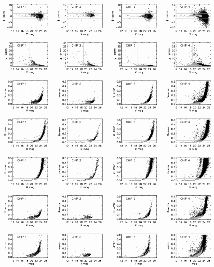
Figure 1: Photometric accuracy and goodness of DAOPHOT fit-to-PSF parameters of targets in our IC 1613 catalogue (black dots) as a function of magnitude. Sources registered at different chips of the WFC are plotted in different columns. The catalogue’s faint limit is V=25. V-magnitude errors for $\rm V\leq 23$ stars are smaller than 0.1. Grey dots are the input set of targets for the search of OB associations. The horizontal lines in the UBV-errors, #- and $\rm\chi$-parm. plots represent the quality requirements explained in Sect. 5.1.1.

The S/N achieved for an apparent magnitude of V=23 is: 21 / 52 / 37 / 27 / 14 for UBVRI respectively. As we show in the next Section, the maximum V-magnitude error for a V=23 star is 0.1. The average full-width half-maximum (FWHM) of point sources is 3.5 / 3.2 / 2.8 / 2.6/ 2.6 pixels for UBVRI i.e., 0.86″-1.16″. At the distance of IC 1613, 1″  is equivalent to 3.5 pc.

Table 1: Log of INT-WFC observations of IC 1613

RA	DEC	T $\rm{}_{exp}\left[\times 100s\right]$					Date
(J2000.0)	(J2000.0)	U	B	V	R	I
01:04:48.4	02:07:10	0.6	0.6	0.6	0.6	0.6	2006/07/30
01:04:48.4	02:07:10	6	3	3	3	3	2006/07/30
01:04:50.4	02:07:40	6	3	3	3	3	2006/07/30
01:04:46.0	02:06:35	6	3	3	3	3	2006/07/30

Complementary VLT-VIMOS images were used for inspection purposes. The observations are the pre-imaging part of programme 078.D-0767, Principal Investigator A. Herrero.

2.1 Photometric Reduction

The photometric reduction was kindly performed by P. Stetson. The data were first corrected for non-linearity, following the prescriptions given in the web page of the WFC. Standard IRAF routines were then used for bias and flat field correction (Valdes, 1997). No defringing mask was applied to the I band images since no reliable map could be obtained from this dataset.

The source extraction was performed on the four chips independently. The DAOPHOT/ALLFRAME software package (Stetson, 1987, 1994) was used according to the following protocol. A first search for stellar sources and aperture photometry was performed on each individual exposure. To build the list of stars suitable to model the point-spread function (PSF), bright and isolated stars with small photometric errors and good shape parameter ( sharpness, hereafter #-parm. ) were selected from the catalogue of extracted sources. An average of 100 to 200 stars were picked per chip, spread throughout its surface to properly model the PSF spatial variations.

Allframe then requires two input files: a list of stars and the geometric transformation needed to match different frames. The latter was estimated using daomatch/daomaster. A new input list of stars was extracted from the median-stacked image (built from all exposures and all filters). Allframe was run once again. Adopting the more accurate stellar centroid and magnitude determinations by allframe enables (i) a better model of the PSF, (ii) a refinement of the geometrical transformation, and (iii) a better median image.

As a by-product, allframe creates individual residual images after source extraction. Visual inspection of the median stack of these, revealed that many stars were missed in the first search, especially in the central region of the galaxy where crowding is quite severe. A second search of stars was performed and the new targets were added to the input list of stars of allframe, which was run a second time with updated PSF and geometrical transformation. This loop (allframe – inspection of the median of the subtracted images – update of input list) was iterated a third and a fourth time for chip 4, that contains the bulk of IC 1613.

Finally, the photometric calibration was performed using local standards from P. Stetson’s catalogue .

The resulting catalogue has almost 85,000 targets. It will be publicly available on-line, with an accurate astrometric calibration for the target coordinates (see Sect. 3). The photometric depth and typical accuracy of the catalogue can be seen in Fig. 1.

The expected foreground contamination in the central $\rm 15\arcmin\times 15\arcmin$ of IC 1613 is $\sim$400 stars with $\rm V\in[16,24]$ and B-V$<$0.8 (Ratnatunga & Bahcall (1985) from the Milky Way model of Bahcall & Soneira (1980)). This region, covered mainly by Chip 4 and marginally with Chips 1 and 3, contains approximately 23,500 objects of our catalogue with the same magnitude and color-range. Foreground contamination is therefore expected to be negligible in the centre of the galaxy. Chip 2 covers the outskirts. It is the least populated and contains only 235 entries in the listed magnitude and color range. Even though a large population of RGB stars is expected in this location (Battinelli et al., 2007), Chip 2 is likely dominated by foreground stars.

3 ASTROMETRIC CALIBRATION FOR WFC IMAGES

The importance of an accurate astrometric solution for any kind of source catalogue is often underestimated. Firstly, it is essential for cross-identification with other existing and future databases, allowing the combined use of complementary data. Secondly, it enables follow-up observations with instruments demanding high position-accuracy, such as multi-object spectrographs. Additionally, instruments with a large field of view (such as the INT-WFC) suffer from large geometric distortions. Our astrometric calibration ensures that the instrumental defects on the target positions are totally removed.

Figure 2: Stacked position residuals of the complete INT-WFC mosaic. The arrows represent the difference between the positions listed by 2MASS and our catalogue, for the reference stars. The scale vector of 1″size is plotted on the lower right corner. A radial correction plus a global cubic polynomial solution has been applied to our catalogue. The positional differences vary as a function of the mosaic coordinates x and y. The fixed pattern shows that instrumental distortions have not been completely removed.

Typically, the transformation from instrumental coordinates into celestial coordinates is accomplished by describing the instrument focal plane with a polynomial model. An existing reference catalogue is used to determine the parameters of the model, i.e. the coefficients of the polynomial. A significant overlap of stars between the observations and the reference catalogue is needed in each exposure, to ensure that the model is well constrained. The solution is then applied to all (x,y) detections, yielding celestial coordinates for all observed objects and not only for the reference stars.

The routine we used for astrometric calibration is fully automatic and does not require a previous manual cross-identification of the observed stars in the reference catalogue. The programme first makes a preliminar cross-identification matching geometrical patterns of both input lists of stars (the measures and the reference one) in the frame’s coordinate system. A linear transformation is calculated and applied to all stars. A new cross-identification is made, this time only searching for positional matches with a tolerance of $0\aas@@fstack{\prime\prime}5$. This way, a more complete list of common stars is achieved. They are used as reference stars to calculate the final solution, a full cubic polynomial transformation. A more detailed description of the procedure is provided in Cabrera-Lavers et al. (2006).

In this work, the reference positions were taken from the 2MASS Catalogue (Cutri et al., 2003) whose reference system is already on the International Celestial Reference System (ICRS). The 2MASS Catalogue does provide a dense reference list of targets with precise positions. Proper motion correction was not necessary since our observations and 2MASS’ are contemporary. Since 2MASS is an infrared survey, we cross-correlated our catalogue’s R magnitude with the J magnitude of 2MASS. The starting point was the instrumental (x,y) positions derived from the PSF fitting described in Section 2.1.

3.1 Mosaic System and Distortion Removal

Figure 3: Stacked position residuals as a function of the chip coordinates (x,y) after radial correction. The $0\aas@@fstack{\prime\prime}1$ size vector is plotted on the lower right corner of the panels. Only a linear characterization of the detector is calculated and applied. The fixed pattern shows that an additional correction is still needed, and that the correction is different for each CCD. Similar plots for Chip 1 and Chip 2 present different distortions.

Detectors with field curvature introduce geometric distortion into the images. The image will experience magnification to a factor that depends on the distance to the optical axis. The resulting radial displacement is usually proportional to $r^{3}$, although perfect azimuthal symmetry is not always seen. This effect must be corrected prior to any celestial coordinate calculation.

It is often found in the literature that the radial distortion of the INT-WFC is removed by following the instructions given in the instrument web page. It suggests performing a radial correction with origin in the optical center of the mosaic (i.e., the composition of the four chips) to calculate a polynomial solution afterwards.

We first transformed the instrumental (x,y) coordinates of all targets on all CCD into global mosaic system $\rm(x_{m},y_{m})$ coordinates with origin in the optical center, using the linear equations:

$$\left\{\begin{array}[]{l}\displaystyle x_{m}=a*x+b*y+c\\ \displaystyle y_{m}=d*x+e*y+f\end{array}\right.$$ (1)

where the $a\,b\,c\,d\,e\,f$ coefficients for each CCD were taken from the technical reports on the WFC.

The radial correction to the coordinates $\rm(x_{m},y_{m})$ is defined as follows:

$$\Delta x=R\ x_{m}\ (x_{m}^{2}+y_{m}^{2})\\ \Delta y=R\ y_{m}\ (x_{m}^{2}+y_{m}^{2})$$ (2)

where R=$\rm-5.30\times 10^{-10}\,pixel^{-2}$ is the distortion coefficient.

After the radial correction was applied, we used a general cubic polynomial solution to describe the detector, as explained in the previous Section. We chose a third-degree polynomial so additional distortions could be accounted for.

Figure 4: Difference between our catalogue and 2MASS positions for the reference stars, as a function of R-magnitude. Upper panel: difference in right ascension. Lower panel: declination differences. The dark line represents the standard deviation.

The residuals of the reference stars are the difference between the transformed instrumental positions and the reference catalogue coordinates. In Figure 2 we have plotted the vector field of residuals as a function of position in the focal plane. A fixed pattern geometric distortion is still present in the INT-WFC system. After several failed tests, we concluded that the combination of a global mosaic radial correction and a subsequent general polynomial solution cannot fully correct the distortion caused by this telescope-camera combination.

The reason why our characterization failed is that each chip demands a different correction. Figure 3 shows that after correcting for radial distortion systematic errors remain in the relative positions (as expected) but each CCD presents a very different pattern of distortion. Hence, for a more accurate calibration we deviated from the generally adopted strategy: after correcting for radial distortion, we estimated an individual fourth-degree polynomial solution for each chip as opposed to calculating a global solution for the whole mosaic system.

3.2 Results and Error Estimate

We estimate the uncertainty of our calibration by comparing our final catalogue with a high precision one: 2MASS. We plot the difference between our positions and 2MASS’ in Figure 4, as a function of the R-magnitude of the targets. The difference between both catalogues is larger in fainter objects but the average is zero, as expected. The standard deviation of the difference is a more meaningful parameter. If the complete catalogue is considered, the standard deviation is ($\sigma_{\alpha cos\delta},\sigma_{\delta})$ = (0$\aas@@fstack{\prime\prime}$19, 0$\aas@@fstack{\prime\prime}$16). Note that the standard deviation is larger (0$\aas@@fstack{\prime\prime}$5) when a global solution for the whole mosaic is calculated. The number of reference stars in each CCD is 140, 123, 138 and 206 stars, respectively.

Let us also remark the lack of any magnitude trend of the differences: the standard deviation increases for faint objects, but the average is always $\sim$0. This fact evidences that the positions obtained are free of any obvious “magnitude equation”, the undesired correlation between the target position relative to the image center and the magnitude of the target. We also investigated the dependence of position difference versus color, and no systematic difference was found.

4 AUTOMATIC SEARCH OF OB ASSOCIATIONS

Catalogues of extragalactic OB associations meant as clustering of bright blue stars over a haze of field stars can already be found in the first extragalactic photographic jobs. However, marking OB associations ’by eye’ is a subjective procedure; the results, namely the sizes of the found associations, depended on a number of factors: distance to the galaxy, plate scale, exposure time and selection criteria (see discussion of Hodge (1986)).

The advent of CCDs combined to target extraction routines (such as DAOPHOT) has given rise to the automatic search of OB associations. The algorithms usually follow two main philosophies: (i) search for statistically significant peaks (over 2 or 3 $\sigma$) in maps of stellar density (Kontizas et al., 1996; Gouliermis et al., 2003) or (ii) the Path Linkage Criterion Method (Battinelli, 1991) also known as friends-of-friends algorithm. The use of pattern recognition (Feitzinger & Braunsfurth, 1984) is less common.

We have developed an algorithm based on the friends-of-friends method: two stars belong to the same association if the distance of one star to the next is less than a given amount. The input entries to the code are a list of points with spatial coordinates and two free parameters, the search distance ($\rm D_{S}$) and the minimum number of members ($\rm N_{min}$) for a group to be considered an association.

Given an OB star, the programme looks for other OB targets within the search distance and registers them as members of the same association. The search is repeated for all the new OB members until no star is found within $\rm D_{S}$  from any of the peripheral stars. In the process, non-OB stars are also included in the association if they are less than $\rm D_{S}$  away from an OB member. Groups with less than $\rm N_{min}$  OB members are discarded.

The one case the algorithm would not detect is a chain of stars each closer to the next less than $\rm D_{S}$  forming a ring of radius larger than $\rm D_{S}$. The code would walk the ring and miss the central targets. At the moment, this has to be checked visually.

There is no physical constraint for the parameters $\rm D_{S}$  and $\rm N_{min}$. In fact, friends-of-friends users do not agree on how to decide their values. $\rm N_{min}$  is more problematic, since the expected population of an association depends on the mass of its parent cloud and the IMF. Borissova et al. (2004) decided $\rm N_{min}$  upon evaluating the chances that an association is actually an accidental group of stars. Other works consider that an OB association is valid if its stellar surface density ($\Sigma$) is statistically above the mean, and choose $\rm D_{S}$  and $\rm N_{min}$  on these grounds. Ivanov (1996) uses $\rm D_{S}$  that maximizes the mean normalized fluctuation of $\Sigma$. Wilson (1991) sets $\rm D_{S}=1/\sqrt{(}\pi\times\Sigma)$ and $\rm N_{min}$  by comparison of the resulting associations to a random area of the galaxy. Georgiev et al. (1999) find $\rm D_{S}$  and $\rm N_{min}$  from the Fourier transform of the surface stellar density.

In this work we infer $\rm N_{min}$  from Milky Way associations, by counting the members observable if they were located at the distance of the studied galaxy (see Sect. 5.2). For $\rm D_{S}$, we follow Battinelli (1991) and Battinelli & Demers (1992) and set this parameter to the abscissa of the maximum of the function $f_{N_{min}}(D_{S})$, the number of associations that the algorithm finds with at least $\rm N_{min}$  stars when run with search distance $\rm D_{S}$. At larger $\rm D_{S}$  associations tend to merge into a single larger system. On the other hand, if $\rm D_{S}$  is small then the associations separate into their individual components (isolated stars or binaries). We adopt this criterion because it is reproducible, but we stress that it does not guarantee that the groups found in this way correspond to physical associations. Note that the visual identifications of OB associations already encountered this problem, and deciding whether a star clustering is only one association, or it can be split into two or more smaller ones was quite arbitrary (Hodge, 1978). Hodge (1986) already pointed out that additional information is required to make sure that we are dealing with physical groups. In fact, the same problem is found when defining OB associations in the Milky Way.

Bastian et al. (2007, 2009) have recently shown that there is a correlation of the typical size of the associations found by friends-of-friends algorithms and the $\rm D_{S}$  value used. These results stress the fact that the OB associations identified this way are not necessarily bound physical entities. Nonetheless, enclosing OB stars in groups is a useful and necessary first step to study the youngest galactic population. Further work studying the color-magnitude diagrams of the associations found in this work (Garcia et al., in prep.) will allow us to progress towards the identification of the real associations.

5 OB ASSOCIATIONS IN IC 1613

The catalogue of OB associations was made in 3 steps. We firstly built an input catalogue of candidate OB stars (Sect. 5.1). Values for the two free parameters of the code, $\rm D_{S}$  and $\rm N_{min}$, were decided afterwards (Sect. 5.2). Finally, the code was run to produce the list of associations, which we inspected individually (Sect. 5.3).

5.1 Input Catalogue of Stars

Table 2: Photometric-quality requirements for stars to enter the algorithm.

V-mag	$\rm\#$-parm.		$\rm\chi$-parm.		error(U, B, V)
	MIN	MAX	MIN	MAX	MAX
$\leq$ 19.0	-2	2	0.5	30	0.05
$>$ 19.0	-2	2	0.5	4	0.05

The starting point is the deep photometric catalogue described in Sect. 2. We kept only stars with exceptional photometric quality, setting hard constraints on the errors of U, B and V magnitudes. The reason is that we built the list of likely OB stars in IC 1613 based only on their reddening-free Q color (see below), a linear combination of U, B and V. If allowed errors in these magnitudes were as large as 0.1, the resulting Q error would be 0.2 and could lead to target mis-classification. We required errors smaller than 0.05 magnitudes. Note that by setting hard constraints on UBV, we do not include the red population with faint U magnitudes (and large U-errors).

We set looser constraints on the DAOPHOT parameters that describe the goodness of the PSF extraction of each target. We allowed for a #-parm. interval (roundness of the PSF) of $\rm[-2,2]$. The $\chi$ parameter (quality of the PSF fit, hereafter $\chi$-parm.) increases with magnitude and tight constraints on this parameter may leave out the brightest stars. In fact, two trends of the $\chi$-parm. are seen in Fig. 1, corresponding to the long and the short exposures. DSS, GALEX and/or VIMOS images reveal that most of the faint targets with $\rm\chi>5$ are background galaxies or blends. A very small fraction corresponds to stars that saturate. We will allow for $\rm\chi\leq 4$ for faint stars, and $\rm\chi\leq 30$ for bright targets.

The photometric qualification criteria are summarised in Table 2. Fig. 1 shows the typical photometric errors of the complete catalogue (black), with the targets that comply with the photometric requirements marked in grey. From a total of 84,771 targets in the initial catalogue, we keep 3,960.

5.1.1 Candidate OB Stars

Candidate blue massive stars were chosen from their Q color, the reddening-free parameter $Q=(U-B)-0.72\times(B-V)$. Q increases monotonically towards later spectral types in the interval $\rm Q\in[-1.0,-0.4]$, corresponding to O3-A0 supergiants and O3-B5 dwarfs (see for instance the calibration of Fitzgerald (1970)). We defined the locus of O and B stars in the U-B vs Q  diagram (Fig. 5) using the colors of stars with spectral types determined by Bresolin et al. (2007). While Q is an indicator of spectral type, U-B holds the information of whether the star is reddened or not. Most O and B supergiants are found in unreddened boxes with $\rm Q\leq-0.4$. IC 1613’s known WO is found in the diagram as an outlier in the lower-left corner.

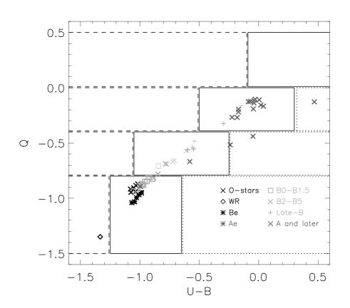
Figure 5: Locus of O and B stars in the U-B vs Q diagram. For each Q-interval delimited by a horizontal band, the central box corresponds to unreddened or moderately reddened objects. The symbols represent stars of different spectral type (from Bresolin et al. (2007)) as detailed in the legend. Most O stars and B supergiants are found in the central unreddened box of the two bottom strips.

Q was the only selection criteria to find OB stars. We allowed for wide ranges of U-B and B-V to account for reddening since we suspect that IC 1613’s internal extinction is not negligible, particularly for OB associations, and that the dust content may be significant in the bar (see full discussion in Sect. 5.1.2).

The allowed V interval is $\rm V\in[16,24]$. This range ensures that all the interesting targets for our spectroscopic studies are included: O3 I/B0 V types, with $\rm M_{V}$=-6.5/-3.8 (Massey, 1998). At the adopted distance modulus DM=24.27, the observed magnitudes will be V=17.8/20.5. We allow for extra 1.5 magnitudes in the bright interval limit, not to leave out exceptional cases such as hypergiants. The limit for faint stars is also extended to allow for reddening and include dwarfs of later B-types.

Table 3 summarizes the photometric properties of candidate OB stars. The photometric constraints set on non-OB stars are listed in Table 4. This is not an attempt to determine the exact spectral sub-types of OB stars from Q. The degeneracy of blue massive star colors at optical wavelengths may be broken in the future with improved photometric capabilities combined with new statistical techniques (Maíz-Apellániz, 2004), but the required accuracy (one thousandth of a magnitude) is not feasible to date.

Table 3: Photometric constraints for OB stars

Parameter	MIN	MAX
V	16	24
Q-parm	-2.0	-0.4
U-B	-2.0	2.0
B-V	-0.5	2.0

Table 4: Photometric constraints for non-OB stars

Parameter	MIN	MAX
V	16	24
Q-parm	-0.4	1.0
U-B	-2.0	2.0
B-V	-0.5	2.0

We note here that the use of the Q parameter has two caveats. (i) It is reddening-independent as long as the reddening law is standard. (ii) Beyond very early spectral types the univocal behaviour of Q cannot be ensured. At Q$\sim$-0.4, it varies rapidly with spectral type and luminosity class. The inherent scatter of the calibration of Q with spectral type may take mid/late B dwarfs and late-B/early-A supergiants to values larger than -0.4. This is the case for the three “late-B” stars in the Q$>$-0.4 box of Fig. 5. Late stars around G-type are close to a local minimum of the Q vs spectral type relationship, at Q$\sim$-0.37. The scatter of the calibration or specific stellar properties (UV excess from stellar activity, for instance) may bring the stars to the boxes of the early types. Finally, Bresolin et al. (2007)’s A8 (A2 Ia) is also in the Q$<$-0.4 locus of B stars. The authors found $\rm H_{\alpha}$ and $\rm H_{\beta}$ P Cygni profiles, and their published spectra shows that the Balmer lines in the blue and near-UV are unusually weak. Clearly, this star is peculiar and hence not expected to follow the general trend.

Table 5: Brightest candidate OB-stars: magnitude and colors. Column ’ASSOC’ indicates the association the stars belong to as found in this work (-1 means they are isolated). We also provide identification numers and spectral types from Bresolin et al. (2007), when available.

ID	RA$\rm[deg]$	DEC$\rm[deg]$	V	B-V	U-B	Q	ASSOC	Bresolin et al. (2007)
	(J2000.0)	(J2000.0)						ID	SpType
39916	16.194780	2.166142	16.43	0.54	-0.05	-0.44	-1	C12	G2
59802	16.246347	2.154164	16.44	0.12	-0.58	-0.67	127	A8	A2 Ia
83197	16.369705	2.083662	16.67	0.19	-0.51	-0.64	-1	-	-
52033	16.224657	2.119503	17.24	0.63	-0.02	-0.47	-1	-	-
62390	16.253813	2.178189	17.42	-0.14	-0.98	-0.88	137	A10	B1 Ia
69336	16.276543	2.158706	17.69	-0.15	-0.98	-0.87	185	B3	B0 Ia
15779	16.124454	2.051565	17.76	0.64	-0.10	-0.56	-1	-	-
42294	16.200409	2.079537	17.95	0.65	0.01	-0.46	60	-	-
65875	16.264278	2.162671	18.06	0.01	-0.55	-0.55	161	A11	B9 Ia
1705	16.023046	2.209241	18.13	0.44	-0.16	-0.48	-1	-	-
60449	16.248133	2.154477	18.23	-0.13	-0.97	-0.88	127	B4	B1.5 Ia
56665	16.237545	2.084683	18.24	0.37	-0.41	-0.68	114	-	-
23263	16.151031	2.190748	18.24	0.39	-0.24	-0.52	-1	C5	A V
58040	16.241360	2.096872	18.39	-0.09	-0.88	-0.82	120	A7	B2 Iab
27381	16.163216	2.146994	18.42	-0.07	-0.88	-0.83	-1	-	-
68599	16.273815	2.096740	18.54	-0.09	-0.85	-0.78	-1	B13	B5 Iab
65133	16.261927	2.083119	18.56	-0.05	-0.70	-0.66	163	-	-
52841	16.226801	2.136780	18.62	-0.07	-0.72	-0.67	105	A5	B3 Ib
34964	16.182615	2.112548	18.62	-0.13	-1.04	-0.94	43	B11	O9.5 I
18570	16.135248	2.158957	18.68	-0.13	-0.94	-0.85	21	C6	B1 Ia

We find that the candidate OB stars concentrate in Chip 4, mostly on the NE lobe of the galaxy where the giant bubbles are seen, but also in the opposite direction, in the SW side of the giant H i cavity where part of the galaxy is enclosed. This is in agreement with previous results (see Sect. 1). Despite our large allowance for V, U-B and B-V to include the most reddened targets, we find very few blue stars in the bar.

The 20 brightest blue stars from our catalogue of OB candidates are listed in Table 5. Spectral types are known for 12 of them. This subset includes an A dwarf and a G2 star (the two “A and later” stars with Q$\rm\lesssim$-0.4 in Fig. 5), which are foreground objects according to Bresolin et al. (2007). It is remarkable that only one red star has entered Table 5, supporting our color selection criteria. Despite its red intrinsic colors the G2 star is in the limit of the accepted Q interval, justifying the need of hard constraints on the photometric errors of stars. The remaining 10 targets (3 of them brighter than V$<$17.8) are O, B and A supergiants, with high chances of been IC 1613 members. Table 5 supports our selection method and also indicates that the foreground contamination is small.

5.1.2 Variable Extinction and Extinction Map

The foreground extinction towards IC 1613 is remarkably low (E(B-V)$\sim$0.2, see Sect. 1). In the past it was argued that the internal reddening was also negligible since background galaxies can be seen through IC 1613 (Hodge, 1978; Freedman, 1988; Krienke & Hodge, 2000), although Hodge (1978) already marked the position of $\sim$10 possible dust clouds in the galaxy.

More recent papers yield higher values of extinction in the lines of sight of individual objects. Humphreys (1980) derived E(B-V)=0.05-0.10 towards early type members, and $\sim$0.2 towards M-supergiants. The cepheid studies of the OGLE (Willick & Batra, 2001) and Araucaria (Pietrzyński et al., 2006) projects yield average extinction values towards their targets of $<$E(B-V)$>$= 0.085 $\pm$0.052 and 0.090$\pm$0.019, with extinction law similar to the MW. Tautvaišienė et al. (2007)’s study of three M-supergiants yields three different values E(B-V)=0.04, 0.06 and 0.03. In the bubble region, Georgiev et al. (1999) report E(B-V)=0.06 and Lozinskaya et al. (2002) finds E(B-V)  in the range of 0.18-0.4 towards 9 OBA stars, considerably larger. The extinction towards the WO is 0.1 (Lee et al., 2003), but reddening is suspected to be high and anomalous towards Wolf-Rayets. Detections of the molecular cloud, neutral hydrogen and dust by IRAS and Spitzer in the bubble region (Meaburn et al., 1988; Jackson et al., 2006) are further evidence of extinction in the area.

Figure 6: Extinction distribution towards the blue massive star candidates of IC 1613. Foreground reddening has not been corrected. Most of the stars have E(B-V)  in the range 0.05-0.25 and the peak of the distribution is located at 0.10-0.15, significantly higher than the published foreground extinction.

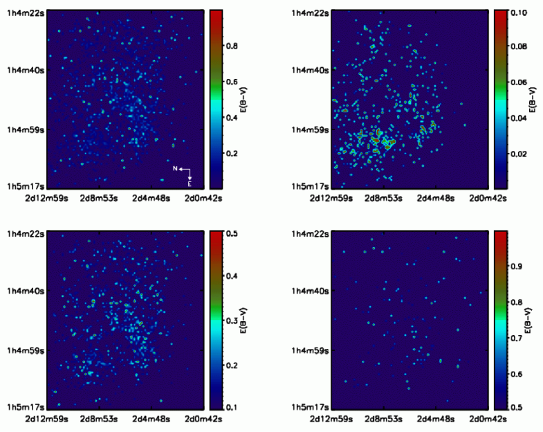
Figure 7: Extinction maps. Only the portion of IC 1613 containing OB associations is shown (same as in Fig. 9). Different panels consider different E(B-V)  ranges. Clock-wise starting from top-left: (1) complete range 0.-1.0, (2) the traditionally considered range for this galaxy 0.-0.1, (3) intermediate E(B-V)  range 0.1-0.5, and (4) large extinction 0.5-1.0.

We therefore suspect that internal reddening is highly variable and far from negligible. To prove it, we have estimated the color excess in the lines of sight of our candidate OB stars in IC 1613. Intrinsic colors were calculated from Q, thanks to its univocal relation with spectral type (hence $\rm(B-V)_{0}$) that holds for the early-type stars. This relation was parameterized for low-metallicity stars by Massey et al. (2000):

$$(B-V)_{0}=-0.005+0.317\times Q$$ (3)

using Kurucz’ ATLAS9 Z=0.08Z_⊙ models. (No such relationship exists for metallicity as low as IC 1613’s, as far as we know). This is an approximation, since equation 3 does not hold if the reddening law deviates from the standard behaviour. Another limitation of equation 3 is that it is independent of luminosity class. Although convenient for fast calculations, it will yield $\rm(B-V)_{0}$ slightly bluer than the actual intrinsic colors of supergiants and slightly redder for dwarfs. The effect will have a maximum for B-type stars. For instance, the comparison of the E(B-V)  provided by Bresolin et al. (2007) for seven early-B supergiants (0.06 on average) with the values derived from equation 3 (0.15 on average), hints that the latter overestimates extinction for these stars. However, we expect that statistically these effects will compensate in the large stellar population of the galaxy.

The distribution of the extinction towards the blue objects of IC 1613 is shown in Fig. 6. It peaks in the E(B-V)  interval 0.10-0.15. Most of the stars have color excess ranging 0.05 to 0.25, higher than the foreground extinction provided in the literature. For a few objects we obtain E(B-V)$>$1. Most of them (more than 90%) are background galaxies for which equation 3 does not apply, and have been discarded. The negative values of E(B-V)  in Fig. 6 are due to a combination of factors, mainly the intrinsic scatter of the calibration of the Q parameter with $\rm(B-V)_{0}$, but also local changes in the slope of the reddening law or photometric errors.

The spatial distribution of E(B-V)  is shown in Fig. 7. The different panels are the extinction maps for 4 different extinction intervals: the complete range (0.-1.0), the traditionally considered range for this galaxy (0.-0.1), intermediate interval (0.1-0.5), and large extinction (0.5-1.0). Starting from the pixel map of the INT-WFC Chip 4 image, stars were distributed into boxes of $\rm 25\times 25$ pixels. Each box was assigned the average extinction of the enclosed stars with E(B-V)  in the studied range. Empty boxes (i.e., bins with no stars with E(B-V)  in the considered interval) where assigned the minimum of the interval. In the 0.-1.0 and 0.-0.1 panels, empty boxes are assigned the minimum positive value found in the sample E(B-V)=0.0002.

Boxes with E(B-V)  in the range 0.-0.1 trace well the star forming regions of the galaxy, which is also the preferred location of OB star candidates. A concentration of E(B-V)$\sim$0.1 points is seen at the bubbles and at the SE edge of the galaxy. Points with larger extinction values (0.1$<$E(B-V)$<$0.5) also trace the star forming regions, with a slight concentration towards the bar area and the SW part of the H i cavity. Larger E(B-V)  values are distributed almost randomly throughout the galaxy. These results support that extinction is not uniform, with rapid spatial variations.

5.2 Free Parameters of the Code

We followed the procedure described in Sect. 4 to determine $\rm D_{S}$  and $\rm N_{min}$.

We used Humphreys (1978)’s catalogue of Galactic OB associations to estimate $\rm N_{min}$. We removed all luminosity class-V stars with spectral type later than B5. ( According to the V-magnitude limits of Table 3 the catalogue of OB candidates would include spectral types down to B8 V, but the Q constraints set the cut at B5 V). 25 out of 78 associations (i.e., $\sim$30%) are left with 3 or less OB members. Since projection effects may be at work, we consider that 2 members are too few for an extragalactic OB association. We therefore set the minimum number of stars to 3, at the risk of neglecting the less massive associations. We expect that we will be able to spot out false OB associations through inspection of the images, and the color-color and color-magnitude diagrams.

We ran the code for different search radii in order to assess $f_{N_{min}}(D_{S})$ (see Fig. 8), and set $\rm D_{S}$  to the abscissa of the maximum. Besides $\rm N_{min}$=3, we tested three additional values: $\rm N_{min}$=4, 5 and 6. The bump of $f_{N_{min}}(D_{S})$ flattens as $\rm N_{min}$  increases, but, in the four cases there is a local maximum at $\rm D_{S}$=6-7″. This local maximum is preserved up to $\rm N_{min}$=10 (not shown in Fig. 8).

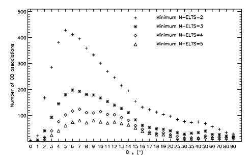
Figure 8: Number of OB associations found as a function of $\rm D_{S}$  and $\rm N_{min}$, $f_{N_{min}}(D_{S})$. Note the irregular scale on the x-axis. Different symbols represent the results for different values of $\rm N_{min}$  as indicated in the legend. There is a local maximum around $\rm D_{S}$=6″. The slight increase at $\rm D_{S}$=50″  is caused by stars in the galactic outskirts, far away between them, that cluster because of the large $\rm D_{S}$  admitted value.

We therefore set $\rm D_{S}=6\arcsec\;and\;N_{min}=3$.

$\rm D_{S}$=6″  is similar to the values derived by Borissova et al. (IC 1613, 6.6″) and Pietrzynski et al. (NGC 300, 7.7″), and much larger than those adopted by Bresolin et al. (1996, 1998, 0.83 to 3.9″  in different spiral galaxies at $\sim$10 Mpc). Since Borissova et al., Pietrzynski et al. and this work have used 2m-class ground-based telescopes with comparable instrumentation whereas Bresolin et al. used HST-WFPC2 data, it is tempting to interpret the differences in terms of the superior plate scale of the WFPC2 (0.1″/px) breaking the OB associations into smaller pieces. However, the physical values of $\rm D_{S}$  vary between the 21 and 23 pc obtained by Borissova et al. and ourselves for IC 1613 and the 35-84 pc obtained for spiral galaxies by Bresolin et al. and Pietrzynski et al. Therefore, the smaller angular value of $\rm D_{S}$  obtained by Bresolin et al. is a consequence of the longer distances towards their sample galaxies (hence smaller angular diameter of associations). Whether the smaller physical values found for IC 1613 are due to inherent differences of star forming regions of irregular galaxies versus spirals, the distance to the galaxies or to poor statistics must be clarified in future works. In the light of Bastian et al. (2007)’s results we also anticipate that the different $\rm D_{S}$  values used will result in different typical sizes for the associations, but we leave the discussion on whether or not there exists a universal length-scale of OB associations for a subsequent paper.

5.3 Final OB Association List

We ran our automatic search algorithm on the catalogue of candidate OB stars one last time with $\rm D_{S}=6\arcsec\;and\;N_{min}=3$, and produced the list of OB associations presented in Sect. 6. All stellar groups provided by the code were accepted as valid associations, as long as they have at least 3 valid members (i.e., not background galaxies, blends or bright red objects with Q$\sim$-0.4). Each association was studied thoroughly using images, color-color (B-V vs U-B  and U-B vs Q) and color-magnitude (B-V vs V  and Q vs V) diagrams to discard fake detections. The analysis of these diagrams will be presented in a second paper.

We examined high resolution images of IC 1613 from the HST archive and VLT-VIMOS using the Aladin software (Bonnarel et al., 2000) to discard non-valid association members, find neighboring associations and/or nearby objects that did not enter the input catalogue because of the quality of their detection (poorer than the requirements of Table 2).

We also cross-matched our catalogue with published spectral classification for IC 1613 targets. The known spectral types of association members are provided in Sect. 6.1.

The code finds 198 groups. 5 of these groups are galaxies. After visual inspection, 29 associations were discarded because they did not reach the minimum number of valid members and 47 were marked dubious because we could not assure that they had at least $\rm N_{min}$  isolated blue stars. The remaining 117 groups ($\sim$60%) are bona-fide OB associations.

6 CATALOGUE OF OB ASSOCIATIONS

The list of OB associations built with our code is presented in Table LABEL:T:ASSprop. Their positions are marked on the galaxy in Fig. 9. Zooms into different galactic sectors are provided in Appendix A.3.

The associations with more than 10 OB members are listed in Table 6, as illustration of the complete catalogue. The content of different columns is: (1) OB association identification number. (2) and (3) Right Ascension (RA) and Declination (DEC) of the centre determined from the average of the positions of the OB members, equinox J2000.0 (4) Number of OB members ($\rm N_{OB}$) of the association. (5) Total number of members registered ($\rm N_{TOT}$); note that our photometric selection criteria is biased against red objects because we demand high accuracy in U magnitudes. (6) Quadrant allocation in Fig. 9. (7) Notes: ’Gal’ – the association is actually a galaxy; ’d’ – association discarded because it does not have enough valid members (i.e. visual inspection reveals that some are blends or gas knots); ’?’ – dubious association (associations with a small number of members, with a significant fraction under suspicion of being blends or not blue stars); ’n’ – an entry in Sect. 6.1.

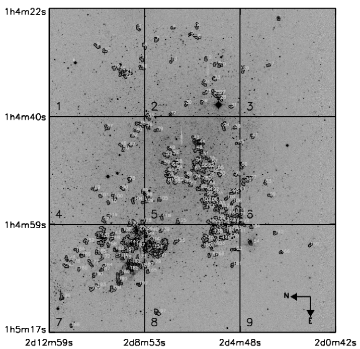
Figure 9: INT-WFC U-band image of IC 1613 (only the portion of Chip 4 that contains the associations is shown). The positions of the associations found in this work are marked in black. The grid divides the image in 9 portions. A zoom into each quadrant is provided in Appendix A.3. Note how the OB associations cluster in sectors 5, 7 and 8.

The code also provides us with a list of the OB members of each association and also the less massive population. Defining OB associations by their members, rather than by hand-drawn lines on photographic plates, allows a direct comparison of results between different works and with observations. The member listings will be available on-line; an example is provided in Table LABEL:T:OBass.

Table 6: OB associations with more than 10 OB-candidate members.

ID	RA $[\deg]$	DEC $[\deg]$	NOB	NTOT	Quad	Notes
	(J2000.0)	(J2000.0)
(1)	(2)	(3)	(4)	(5)	(6)	(7)
151	16.260516	2.140498	99	103	7,8	n
147	16.257084	2.158485	53	58	7	n
127	16.248152	2.153727	49	54	4,7	n
137	16.253227	2.178541	46	48	7	n
135	16.249324	2.097876	31	37	8	-
175	16.270523	2.157452	28	30	7	n
114	16.235155	2.082594	22	23	5,6	n
103	16.229149	2.096880	19	23	5	n
21	16.135528	2.161271	17	18	1	n
185	16.276164	2.158762	17	17	7	n
56	16.203010	2.107146	16	19	5	-
44	16.186156	2.108783	16	17	5	-
88	16.217727	2.107367	16	17	5	-
122	16.242760	2.079217	15	19	5,6,8,9	n
106	16.227180	2.101775	14	18	5	n
123	16.241480	2.089006	14	15	5,8	-
132	16.248173	2.090002	13	14	8	-
191	16.283802	2.166530	13	13	7	n
76	16.213125	2.076123	12	13	6	-
154	16.256969	2.072318	11	12	9	n
161	16.262861	2.161338	11	12	7	n

6.1 Comments on Individual Associations

Assoc. #10: an A3 II (Bresolin et al. (2007)’s C3) is located 6$\arcsec$.2 away from one association member.

Assoc. #16: Part of the association shows radial distribution around one red and two blue central stars, that were not included in the OB catalogue because of their photometric errors.

Assoc. #21: The brightest blue star is a B1 Ia whose spectrum displays strong $\rm H_{\alpha}$  wind emission (Bresolin et al. (2007), id: C6).

Assocs. #27 and #28: their members are horizontally aligned in our images (they have very similar RA), perpendicularly to a spike of a nearby saturating bright star. The brightest stars of both associations fall right on the spike, and we discard them because their photometry may be altered.

Assoc. #43: The brightest star is Bresolin et al. (2007)’s B11, an O9.5 I.

Assoc. #48: Blue stars 7$\arcsec$ away in the SE direction could connect this association with #51.

Assoc. #53: Bresolin et al. (2007)’s C16, an A5 Ib, is included as a red member.

Assoc. #54: A bright blue nearby (8$\arcsec$  away) star is missed for the association.

Assoc. #61: Its brightest member is Bresolin et al. (2007)’s B8 (B8 Ib).

Assoc. #69: The brightest star is Bresolin et al. (2007)’s B10 (B8 Iab).

Assoc. #75 includes an A5 II (Bresolin et al. (2007)’s A2). A nearby red star (not listed under the association) could be a red supergiant (RSG).

Assoc. #83’s brightest blue member has very blue Q. It is a Be star (Bresolin et al. (2007)’s B19); its emission lines may explain its bluer color. Additional faint blue stars are found nearby (at $\sim$ 7″-9″).

Assoc. #85: An additional blue star is only 7″  away.

Assoc. #86: Its brightest member looks triple in the WFPC2 images. A nearby bright red star could be an RSG star of this association.

Assoc. #96: Bresolin et al. (2007)’s A3 (A7-F0 Ib) is only 7″away.

Assoc. #97: Bresolin et al. (2007)’s A4 (B9 II) is only 9″away.

Assoc. #98: An additional blue target 9″  away is missed for the association.

Assoc. #99: A member with very blue Q has the same position in the U-B vs Q diagram as IC 1613’s WO. However, this object may be blended with the brightest association member.

Assoc. #103: Bresolin et al. (2007)’s A4 star, a B9 II, is included in the association. Because of its late spectral type, this object’s Q color is slightly beyond our Q constraint for blue stars (i.e., Q$>$-0.4).

Assoc. #104 contains Bresolin et al. (2007)’s C17 star, an early-A II. The target enters the catalogue as a red star (Q $>$-0.4).

Assoc. #105 contains Bresolin et al. (2007)’s A5 star (B3 Ib). (This association was discarded because it only has 2 valid members).

Assoc. #106: The brightest star is Bresolin et al. (2007)’s A4b star (B5 Ib).

Assoc. #114 is a round association located at the outer part of the galaxy. The brightest blue star (V$\sim$18.5) could be blended with the next two brightest stars of the association, although targets are well resolved in VLT-VIMOS images.

Assoc. #116: A B0 Iab star (Bresolin et al. (2007)’s B14) is close to the association.

Assoc. #117: The position of the red member in the color-magnitude diagrams matches that of an RSG. Close to association #114, together they could form a ring.

Assoc. #120: The brightest member is Bresolin et al. (2007)’s A7, B2 Iab.

Assoc. #122: The brightest blue member is Bresolin et al. (2007)’s B16, B1.5 Iab.

Assoc. #124’s brightest member is an A0 III (Bresolin et al. (2007), id: B15).

Assoc. #125 : Its brightest member could be contaminated by a nearby red star, although its normal colors suggest otherwise.

Assoc. #126: The brightest star has very blue Q and its colors deviate from the reddening law, but visual inspection reveals that it is a normal isolated star. This star is $\rm[AM85]3$, with spectral type OB+em (Azzopardi et al., 1988). The nebular emission could explain its anomalously blue Q.

Assoc. #127 delineates the bright part of one of the bubbles of the NE lobe. #127 may form a single giant association with #147. Spectral types are known for three stars in the association: the brightest blue stars have types A2 Ia and B1.5 Ia (Bresolin et al. (2007)’s id’s are A8 and B4). Skiff (2007) assigns A0 Ia(e) to the former and additionally lists an RSG, $\rm[S71]$V32 with type M1 Ia (not included in our catalogue because of the hard constraints on blue photometric errors). The A-supergiant has been suggested being a foreground star (Sandage & Katem, 1976), but Bresolin et al. (2007) found its radial velocity in agreement with IC 1613, and report P Cygni profiles of $\rm H_{\gamma}$ and $\rm H_{\beta}$ (see Sect. 5.1.1). Spectroscopy of higher resolution than Bresolin et al. (2007)’s VLT-FORS2 data is needed to determine whether this object is an LBV-candidate.

Assoc. #128: The brightest star is a Be (Bresolin et al. (2007)’s B5), and this may explain its very blue Q color.

Assoc. #134: A possible additional member, bright and blue, is only 7″away.

Assoc. #136 marks a bubble rim.

Assoc. #137 is formed by several arc-like structures that possibly trace the edges of several bubbles. Four members at the West could form a separate association. The brightest member is a B supergiant: B1 Ia (Bresolin et al. (2007)’s A10), B2/3 Ie (Skiff, 2007), B2-3 I (Humphreys, 1980). The second brightest star is Bresolin et al. (2007)’s A9 (B5 Iab).

Assoc. #140: A nearby blue star ($\sim$7″  away) is not included in the association.

Assoc. #144: The brightest member ionizes its surrounding nebula.

Assoc. #146: The brightest member is a Be (Bresolin et al. (2007), id: B12).

Assoc. #147 is dominated by 2 clumps, each in the intersection of 2 bubbles, plus 2 arc-like structures that trace the rim of one bubble each. Some detections are actually nebular knots (discarded). The association has 5 bright members ($\rm V\in[19,20]$), four of them in the largest clump of stars. Lozinskaya et al. (2002) obtained low resolution spectra ($\rm\Delta\lambda=$8Å) of the stars in the main clump, with a 6m telescope (note that this area is hardly resolved, even in the VLT-VIMOS images). The group includes an Of star, two O giants and two OB candidates. The association has an additional OB member, far from the regions of crowding (OB+em?, Azzopardi et al. (1988)).

Assoc. #148: A nearby blue star, potential member of the association, is 7.5″away.

Assoc. #149 is in the bubble region, between the large associations #137 and #147, but no nebulosity is seen nearby.

Assoc. #151 is the association with more OB members of our catalogue. It is arc-shaped and part of it follows one bubble. IC 1613’s known supernova remnant (SNR) is included in the association. Our catalogue yields 5 detections for the SNR, which we discard. We note here one apparently isolated target whose position in the Q vs U-B and B-V vs U-B color-color diagrams is the same as for the WO star. Several obscured clouds fall within the limits of the association.

The age of the SNR is yet undecided since it shows both young and old signatures. While it was originally believed to be about 2E4 years old (Dodorico & Dopita, 1983; Peimbert et al., 1988) X-ray observations suggest an age of 3E3 years (Jones et al., 1998). The emission lines from the knots resemble those from the Crab Nebula and Cygnus Loop filaments, indicating that this is a young SNR (Armandroff & Massey, 1991). It has been suggested that the SN exploded inside a large cavity surrounded by a dense H i cloud. The remnant would have just encountered the dense material, producing shocks and hence the peculiar features (Lozinskaya et al., 1998, 2003).

Spectral types are known for three stars in this association. The two brightest blue stars are an O9 I and a B1 Ia, Bresolin et al. (2007)’s B7 and B6. The authors report strong $\rm H_{\alpha}$  wind emission in the spectrum of B6. The association contains a red supergiant, Sandage & Katem (1976)’s variable star $\rm[S71]$V38 (M0 Ia, Skiff (2007)). The RSG is only 6.7″  away from association #150.

Assoc. #154 encloses IC 1613’s known WO star. The object has very blue Q and U-B colors (V=19.86, Q=-1.35, B-V=0.02, U-B=-1.33). The WO is located on the edge of the giant H i shell that contains the SW side of the galaxy, and ionizes an asymmetric bipolar H ii region (Afanas’ev et al., 2000; Lozinskaya et al., 2001). These authors find at least two extra sources in $\rm H_{\alpha}$ and HeII 4686 narrow-band filters that are compact knots of gas. Some entries of our OB candidate list are also knots of the nebula ionized by the WR. They are characterized by very blue Q and red B-V. However, U, B and R VLT-VIMOS images suggest that two of the detections (besides the WO) are in fact stars. One of them has very blue Q, and the other one, very embedded in the WO nebula, has red Q. These stars might be members of a cluster hidden behind the WO, proposed by Lozinskaya et al. (2001). The bipolar shell’s dynamical age is 0.3-1E6 years (Afanas’ev et al., 2000), consistent with the duration of the WR stage.

Assoc. #157: VLT-VIMOS images reveal that the brightest star is triple, and unresolved in our catalogue. One member has similar colors to the brightest star in #158, which has been found to be an LBV-candidate.

Assoc. #158 is located in the void of the bubble region, like #149. One of the members has very red B-V and blue Q. Medium resolution spectroscopy soon to be published (Herrero et al. 2009, in prep.) has revealed P Cygni profiles of the Balmer series and of iron, rendering the target an LBV-candidate.

Assoc. #161 traces two bubble rims, sharing one of them with association #147. The brightest target is Bresolin et al. (2007)’s A11 (B9 Ia).

Assoc. #162’s brightest star is in the intersection with one of the bubble rims followed by #161. Its spectral type is O5-O6 V (Bresolin et al. (2007)’s B2), and it is likely ionizing its surrounding nebula.

Assoc. #175: The association is spatially divided into two parts, one at the centre of a bubble, and the other in the intersection of such bubble and another that encloses association #185. One apparently isolated member has very blue Q ($\sim$-1.4), and its position in the Q vs U-B and B-V vs U-B diagrams is similar to the WO.

Assoc. #176: Two out of its three members are in the centre of a small bubble.

Assoc. #179’s brightest star is Bresolin et al. (2007)’s A12, a B1.5 Iab.

Assoc. #184 is found in the SW outskirts of the galaxy. The stars are distributed in a ring shape, around a central red star.

Assoc. #185: Members are located on the rim of one bubble, but they may also be creating the bubble where part of association #175 is located at the SW. The association has a high stellar density and all members may experience blends. The brightest star is an early B-supergiant (B0 Ia Bresolin et al. (2007)’s B3; B:I: Sandage & Katem (1976)’s B42) although Lozinskaya et al. (2002) classified it as an O supergiant. The study of the latter in this region (see comment on association #147 for a description of their analysis) found 3 more OB stars: O III, B8 II and one with uncertain type O8 III or O4 V . A faint member (V$\sim$22) with extremely blue Q and U-B, sits in the same position in the U-B vs Q  diagram as the WO.

Assoc. #187’s brightest member is Bresolin et al. (2007)’s A13 a very early O dwarf (O3-4 V((f))), which is remarkable for a modest association of only 3 members.

Assoc. #189 is located on the rim of a bubble. The spatial distribution suggests that the H ii shell could have been blown either by association #185 or by a nearby isolated star.

Assoc. #191 is linear in shape and located in the bubble region, close to association #189. The brightest star is a late-O giant (O9 III, Bresolin et al. (2007)’s A15).

Assoc. #196’s brightest star is a Be, Bresolin et al. (2007)’s A17. Their target A16 (early-B Ib) is only 6.1″  away.

7 THE EFFECT OF THE V-FAINT LIMIT ON THE FINAL CATALOGUE OF ASSOCIATIONS

The selection criteria for OB stars were flexible in magnitude and colors to admit very extincted stars, since we suspected that internal reddening was significant. However, after inspecting the associations we have found that the redder faint stars are not reddened blue stars, but mostly non-stellar objects or blends. We consequently wonder how allowing such a large range of V-magnitudes and colors has distorted the resulting catalogue of associations. Fainter stars are more abundant, hence closer to each other, and may shift the value of $\rm D_{S}$  to shorter distances. By setting $\rm D_{S}$  to a short value, we may be missing looser groups of bright OB candidates.

We ran the OB association search programme on a subset of the initial sample: bright stars with V$<$21. The resulting list of associations (hereafter catalogue-B) is compared with our results (catalogue-A) in Fig. 10.

As expected we obtained a longer $\rm D_{S}$=11$\arcsec$ for the less dense group of bright stars. There is good agreement of both catalogues on the bubble NE region of the galaxy. The associations in catalogue-B are usually larger and enclose several associations of catalogue-A. However, the SW side of the galaxy in the H i cavity is apparently dominated by fainter stars, and by limiting ourselves to the brightest ones we would have missed a large number of associations. On the other hand, by enlarging $\rm D_{S}$  to 11″  we would include three more associations. Whether they are real OB associations can only be decided after closer inspection of their stellar content.

We conclude that the criteria used to build catalogue-A favoured the identification of OB associations, although some extra work was needed afterwards to discard fake identifications.

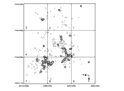
Figure 10: Comparison of the results presented in this paper (catalogue-A, grey shadows) and the results of the OB association search algorithm run on the same sample of stars but V$<$21 (catalogue-B, black). The associations found in both cases agree on the bubble region, but the SW side of the galaxy is dominated by associations with fainter stars. Catalogue-A misses 3 associations of bright stars.

8 COMPARISON WITH PREVIOUS CATALOGUES

Four catalogues of OB associations in IC 1613 have been published to date. The first one was made from visual inspection of plates and published by Hodge (1978). More recent works by Ivanov (1996) (catalogue not public), Georgiev et al. (1999) and Borissova et al. (2004) have used an automatic procedure very similar to ours. Our work has produced the most numerous catalogue: a total of 163 stellar groups, almost triplicating the 60 associations found by Borissova et al. Hodge (1978) listed 20 associations and Ivanov (1996) only found 6. Georgiev et al. (1999) studied a smaller field.

Direct comparison of our results with the seminal work of Hodge (1978) can only be done qualitatively, since his catalogue is marked on low resolution photographic plates of the galaxy. The associations we have found follow the same distribution as Hodge (1978)’s, but our code breaks them into many smaller ones. Georgiev et al. (1999) observed the same effect in their results for the bubble area of the galaxy, and pointed out that their associations are the bright cores of Hodge’s. We also find new associations both at the core of IC 1613 and the periphery. Both facts are explained by the higher sensitivity and finer spatial resolution of this work.

The associations found by Georgiev et al. (1999) are provided on detector coordinates or plotted over a poor quality image, and since the same team studied a wider field in Borissova et al. (2004) we preferred the latter for comparison. We use the coordinates and radius of the associations in their Table 1 to compare with ours (see Fig. 11). We noted a discrepancy between the centres provided in their list and the position of some associations they marked over a picture of IC 1613 in their Fig. 1. By providing electronically the list of OB members of each association, we expect to minimize these kind of inconsistencies and to make direct inter-comparisons easier.

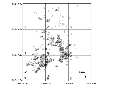
Figure 11: Comparison of the associations found in this work (grey), with those of Borissova et al. (2004) (black). The quadrants mark the same positions as in Fig. 9. The overall distribution of the associations in both catalogues agrees. Considering the associations in the H i cavity, our results separate Borissova et al. (2004) groups at the SE into many pieces. At the NW end, Borissova et al. (2004) find 4 associations (G51,G56,G57,G58) that do not have a counterpart in our catalogue. Other unmatched associations are their G26 and G55.

The overall distribution of our catalogue and Borissova et al. (2004)’s associations agrees. The data they used have a plate scale similar to ours but again, our catalogue separates most of their associations into two or more, especially in the SW part of the galaxy enclosed in the H i cavity (see Fig. 11). Our catalogue has additional associations in the outer reaches of IC 1613, as expected because of our extended field of view, but also in the overlapping areas. The likely reason why these associations were not registered by Borissova et al. is that they do not reach the minimum number of elements considered in their work ($\rm N_{min}$=4). In other cases the members are faint, beyond Borissova et al.’s limiting V-magnitude. These authors found 3 associations (G26, G51, G55) far from any of ours (see Fig. 11); we do find OB stars on those locations, but they are separated more than $\rm D_{S}$  and hence not included in our catalogue. There is also a mismatch between associations G57-G58 and the centre of our counterparts.

The different number of associations found by Hodge (1978), Borissova et al. (2004) and ourselves may be better explained in light of the experiment described in Sect. 7. Hodge only considered stars with V$<$21 to find associations, and Borissova et al. have completeness problems for fainter magnitudes. Catalogue-B consists of 31 associations of average diameter similar to the mean size of the associations of Borissova et al. (2004), decreasing the discrepancies. However, catalogue-B still does not include Borissova et al. (2004)’s associations without counterpart in catalogue-A.

9 SUMMARY AND FUTURE WORK

This paper presents a deep multi-band photometric catalogue of IC 1613 with high astrometric accuracy. Using the univocal relation between the reddening-free Q parameter and OB spectral types, we have built a list of candidate young massive stars. With a friends-of-friends algorithm developed by our group, we have studied how they cluster into associations. A total of 163 associations were found (after discarding 5 galaxies and 29 cases with less than $\rm N_{min}$  valid members), ranging from small groups of 3 stars to large complexes of more than 20 members in the centre of H ii shells. 24 associations have 10 or more OB candidates. Our findings are dependent on the choice of the two free parameters of the friends-of-friends algorithm: the search distance (6″) and the minimum number of OB stars defining an association (3).

The resulting set of candidate OB stars is ready to be observed with multi-object spectrographs. To achieve the required astrometric precision, a new solution for the WFC at the INT was developed.

The photometric analysis leaves an interesting by-product, an extinction map of IC 1613. Most of the OB stars exhibit a color excess larger than the foreground value. Extinction is not uniform and does not have a smooth distribution. The points of enhanced reddening are spread throughout the galaxy and show a slightly higher concentration at the edge of the H i cavity that contains the SW side of the galaxy.

The positive confrontation of our list of candidate OB stars with published spectral types, endorse our target selection criteria based mainly on Q and secondarily on U-B colors. Four stars are found in the same position of the U-B vs Q diagram as the known Wolf-Rayet star of the galaxy.

This article is the first effort towards a comprehensive description of the massive stellar population of IC 1613, as a proxy for the low-metallicity early-Universe. The next step is the characterization of the physical properties of the associations presented here, especially mass and age. The study of the color-magnitude and color-color diagrams of the catalogue associations and their comparison with theoretical isochrones will be presented in part-II. It will provide interesting clues about star formation processes of massive stars and their IMF in low metallicity environments.

Appendix A CATALOGUE OF OB ASSOCIATIONS

A.1 Complete Catalogue

The output list of OB associations provided by our code is presented in Table LABEL:T:ASSprop.

The content of different columns is: (1) OB association identification number. (2) and (3) Right Ascension (RA) and Declination (DEC) of the centre determined from the average of the positions of the OB members, equinox J2000.0. (4) Number of OB members ($\rm N_{OB}$) of the association. (5) Total number of members ($\rm N_{TOT}$); this figure may not be representative since our photometric selection criteria is biased against red objects by demanding high U-magnitude accuracy. (6) Quadrant allocation in Fig. 9. (7) Notes: ’Gal’ – the association is actually a galaxy; ’d’ – association discarded because it does not have enough valid members (i.e. visual inspection reveals that some are blends or gas knots); ’?’ – dubious association (associations with a small number of members, with a significant fraction under suspicion of being blends or not blue stars); ’n’ – an entry in Sect. 6.1.

A.2 Member Listing Example: Association # 16

Our code provides us with a list of the OB candidate members of each association and also the red population. Defining OB associations by their members, rather than by hand-drawn lines on photographic plates, allows a direct comparison of results between different works and with observations. The member listings of all the associations of our catalogue will be available on-line.

As an example, we list the members of association #16 in Table LABEL:T:OBass. The content of different columns is: (1) Star identification number in our catalogue. (2) and (3) Right Ascension and Declination, equinox J2000.0. (4), (6), (8), (10) and (12) magnitudes. (5), (7), (9), (11) and (13) error of magnitude measurements. (14) and (15) DAOPHOT’s $\chi$ and # parameters. (16) Identification number in the 2MASS catalogue.

A.3 Finding Charts of the Associations

The positions of the associations were marked on the galaxy in Fig. 9. Zooms into different galactic sectors are provided in this Appendix, Figs. LABEL:F:f-charts1-LABEL:F:f-charts9.

Table 7: Catalogue of OB associations in IC 1613.

ID	RA $[\deg]$	DEC $[\deg]$	NOB	NTOT	Quad	Notes
	(J2000.0)	(J2000.0)
(1)	(2)	(3)	(4)	(5)	(6)	(7)
1	16.096912	2.052357	8	10	3	Gal
2	16.102215	2.110539	3	3	2	-
3	16.103825	2.152657	4	4	1	-
4	16.103556	2.127854	3	3	2	d
5	16.108092	2.114839	3	3	2	?
6	16.110625	2.110028	3	3	2	-
7	16.112182	2.139603	4	4	2	-
8	16.116793	2.148229	4	4	1,2	-
9	16.116749	2.181977	5	5	1	-
10	16.120176	2.176666	3	3	1	n
11	16.125909	2.149869	4	4	1	-
12	16.125697	2.104176	3	3	2	d
13	16.127069	2.128816	4	4	2	-
14	16.129429	2.097499	4	4	2	-
15	16.130444	2.093961	3	3	2	-
16	16.133370	2.165873	10	12	1	n
17	16.130397	2.059373	3	3	3	-
18	16.132333	2.150075	4	4	1,2	-
19	16.132298	2.169800	3	4	1	?
20	16.133645	2.077595	4	4	3	-
21	16.135528	2.161271	17	18	1	n
22	16.138624	2.161875	3	3	1	-
23	16.140158	2.098123	4	4	2	?
24	16.143162	2.105718	5	5	2	-
25	16.150666	2.098182	7	9	2	d
26	16.149934	2.104582	3	3	2	-
27	16.150782	2.094274	5	5	2	n
28	16.154294	2.093873	4	4	2	n
29	16.156629	2.107164	3	3	2	?
30	16.157865	2.118325	4	4	2	-
31	16.160063	2.086166	3	4	2	-
32	16.165508	2.129537	7	7	2	Gal
33	16.167062	2.145645	5	7	2,5	-
34	16.173860	2.091680	7	8	5	-
35	16.172452	2.151775	8	9	4	-
36	16.173835	2.146373	4	7	4,5	-
37	16.174840	2.174687	4	5	4	-
38	16.174955	2.083569	3	3	5	-
39	16.176810	2.138951	3	3	5	d
40	16.177356	2.153791	3	3	4	?
41	16.181246	2.070946	4	4	6	-
42	16.180837	2.156761	3	3	4	d
43	16.182817	2.112977	3	5	5	n
44	16.186156	2.108783	16	17	5	-
45	16.185969	2.081011	3	3	5,6	?
46	16.187206	2.165141	3	3	4	d
47	16.187683	2.158649	3	5	4	?
48	16.190017	2.110850	9	9	5	n
49	16.189936	2.130523	3	5	5	d
50	16.190243	2.163109	3	5	4	d
51	16.194281	2.106449	8	10	5	n
52	16.193448	2.127703	3	4	5	d
53	16.194693	2.132499	7	8	5	n
54	16.198802	2.111230	9	10	5	n
55	16.197736	2.101776	3	3	5	d
56	16.203010	2.107146	16	19	5	-
57	16.200013	2.100085	4	4	5	?
58	16.200024	2.125184	6	6	5	?
59	16.200528	2.133959	3	4	5	d
60	16.202105	2.078538	6	6	5,6	?
61	16.202044	2.128357	4	4	5	n
62	16.202794	2.102484	3	3	5	d
63	16.204786	2.112106	7	7	5	-
64	16.204397	2.124905	5	5	5	-
65	16.204474	2.095443	4	5	5	d
66	16.205571	2.130890	8	10	5	?
67	16.206485	2.126462	4	5	5	?
68	16.206628	2.099115	3	3	5	?
69	16.209295	2.117948	6	8	5	n
70	16.208526	2.094393	3	3	5	d
71	16.208783	2.083076	3	4	5	d
72	16.209589	2.101978	3	3	5	?
73	16.209537	2.131091	5	5	5	-
74	16.210802	2.111945	3	3	5	d
75	16.211725	2.106787	5	8	5	?n
76	16.213125	2.076123	12	13	6	-
77	16.211226	2.072083	4	4	6	?
78	16.212151	2.158723	4	4	4	?
79	16.211941	2.127620	3	3	5	?
80	16.212032	2.104437	3	5	5	-
81	16.213312	2.131232	3	3	5	-
82	16.213018	2.124339	4	5	5	?
83	16.214367	2.061752	3	3	6	n
84	16.216014	2.101695	10	10	5	-
85	16.213772	2.118912	3	3	5	?n
86	16.214380	2.126652	3	3	5	?n
87	16.215442	2.115048	5	5	5	-
88	16.217727	2.107367	16	17	5	-
89	16.218450	2.183555	6	6	4	-
90	16.218416	2.163930	3	3	4	?
91	16.219528	2.079689	6	6	5,6	-
92	16.219961	2.098888	3	3	5	d
93	16.220890	2.084779	6	7	5	-
94	16.219702	2.103431	4	4	5	?
95	16.220188	2.149358	3	3	4	-
96	16.222186	2.096009	4	5	5	n
97	16.222757	2.103359	3	3	5	n
98	16.223875	2.146328	6	7	4,5	n
99	16.223379	2.058472	4	4	6	n
100	16.224860	2.169550	6	6	4	-
101	16.223822	2.179711	3	3	4	d
102	16.225417	2.089271	3	3	5	d
103	16.229149	2.096880	19	23	5	n
104	16.226815	2.155823	7	10	4	?n
105	16.226303	2.137465	3	3	5	dn
106	16.227180	2.101775	14	18	5	n
107	16.227032	2.107051	3	3	5	d
108	16.227880	2.084607	4	6	5	?
109	16.227894	2.147403	5	5	4,5	?
110	16.228626	2.173969	3	4	4	?
111	16.229030	2.104253	5	5	5	?
112	16.231603	2.093674	3	4	5	?
113	16.231901	2.103999	5	6	5	-
114	16.235155	2.082594	22	23	5,6	n
115	16.233123	2.089860	3	3	5	d
116	16.236758	2.089753	6	7	5	n
117	16.237337	2.079615	3	4	5,6	n
118	16.238855	2.135455	3	3	5	d
119	16.238087	2.173274	3	3	4	-
120	16.240415	2.096584	7	7	5	n
121	16.240945	2.177397	4	4	4	-
122	16.242760	2.079217	15	19	5,6,8,9	n
123	16.241480	2.089006	14	15	5,8	-
124	16.241957	2.084267	7	8	5,8	n
125	16.242312	2.124345	5	5	5,8	n
126	16.243098	2.093806	5	5	5,8	n
127	16.248152	2.153727	49	54	4,7	n
128	16.242096	2.149247	4	5	4,5	n
129	16.242767	2.101736	6	6	5,8	-
130	16.244092	2.158721	4	5	4,7	-
131	16.243844	2.098030	3	3	5,8	-
132	16.248173	2.090002	13	14	8	-
133	16.247413	2.085148	5	5	8	-
134	16.246209	2.071744	3	3	9	n
135	16.249324	2.097876	31	37	8	-
136	16.247844	2.148337	4	4	7,8	n
137	16.253227	2.178541	46	48	7	n
138	16.248630	2.163478	6	6	7	?
139	16.248756	2.136402	3	3	8	d
140	16.248518	2.144179	3	3	8	?n
141	16.249494	2.081922	3	3	8	Gal
142	16.250423	2.054868	4	4	9	-
143	16.250916	2.170979	3	3	7	-
144	16.251720	2.146901	3	3	8	n
145	16.252874	2.086635	9	9	8	-
146	16.254549	2.104795	10	10	8	n
147	16.257084	2.158485	53	58	7	n
148	16.254275	2.092485	6	7	8	n
149	16.254539	2.171786	3	3	7	?n
150	16.255150	2.142742	5	6	8	-
151	16.260516	2.140498	99	103	7,8	n
152	16.256125	2.190009	4	4	7	-
153	16.256249	2.125097	5	5	8	-
154	16.256969	2.072318	11	12	9	n
155	16.258348	2.100803	9	10	8	-
156	16.258377	2.096784	3	5	8	d
157	16.259700	2.153904	4	4	7	?n
158	16.258826	2.173986	3	3	7	?n
159	16.258869	2.029636	3	3	9	Gal
160	16.259788	2.106187	5	5	8	-
161	16.262861	2.161338	11	12	7	n
162	16.262323	2.169053	3	5	7	n
163	16.262203	2.084492	3	3	8	-
164	16.262549	2.196617	3	4	7	?
165	16.264022	2.181578	4	4	7	-
166	16.264283	2.050493	6	6	9	Gal
167	16.266025	2.101659	3	3	8	?
168	16.265918	2.097347	3	4	8	?
169	16.266384	2.192655	4	4	7	-
170	16.266803	2.166934	3	3	7	?
171	16.266873	2.138073	4	5	8	-
172	16.267850	2.178595	3	3	7	d
173	16.268078	2.152881	3	3	7	-
174	16.268225	2.203677	3	3	7	-
175	16.270523	2.157452	28	30	7	n
176	16.268470	2.163499	3	3	7	n
177	16.271771	2.186759	5	5	7	-
178	16.271105	2.200210	4	6	7	-
179	16.271636	2.142294	3	3	8	?n
180	16.273082	2.147837	4	7	7,8	-
181	16.272820	2.084834	4	4	8	d
182	16.273732	2.204206	4	4	7	-
183	16.274270	2.150566	3	4	7	d
184	16.273774	2.177004	3	3	7	?n
185	16.276164	2.158762	17	17	7	n
186	16.275929	2.194830	3	3	7	?
187	16.276569	2.178761	3	3	7	n
188	16.277759	2.145682	4	5	8	?
189	16.278765	2.164795	4	4	7	?n
190	16.280133	2.183874	3	3	7	d
191	16.283802	2.166530	13	13	7	n
192	16.286930	2.151835	3	3	7	?
193	16.288172	2.181669	4	4	7	?
194	16.290408	2.170542	6	7	7	?
195	16.290153	2.185749	4	4	7	?
196	16.295735	2.207267	5	5	7	n
197	16.306976	2.139009	8	8	8	-
198	16.316533	2.200474	3	3	7	d

Table 7: continued.

Non OB-stars in Association    ID RA $\rm[deg]$ DEC $\rm[deg]$ V $\sigma$-V B $\sigma$-B I $\sigma$-I R $\sigma$-R U $\sigma$-U $\rm\chi$ # ID_2MASS (J2000.0) (J2000.0) (1) (2) (3) (4) (5) (6) (7) (8) (9) (10) (11) (12) (13) (14) (15) (16) 16825 16.128596 2.164702 21.332 0.0173 21.617 0.0150 20.855 0.0280 21.120 0.0200 21.678 0.0367 1.266 0.383 – 18116 16.133573 2.166236 21.772 0.0352 22.151 0.0217 21.064 0.0657 21.464 0.0485 22.176 0.0466 1.789 0.661 –