Abstract

The influence of the unlike Lennard-Jones (LJ) parameters on vapor-liquid equilibria of mixtures is investigated and the performance of eleven combining rules is assessed. In the first part of the work, the influence of the unlike LJ size and energy parameter on vapor pressure, bubble density and dew point composition is systematically studied for the mixtures CO+$\rm C_{2}H_{6}$ and $\rm N_{2}$+$\rm C_{3}H_{6}$, respectively. It is found that mixture vapor pressure depends strongly both on the size and the energy parameter whereas the bubble density depends mostly on the size parameter and the dew point composition is rather insensitive to both parameters. In preceding work, unlike LJ parameters were adjusted to experimental binary vapor-liquid equilibria for 44 real mixtures. On the basis of these results, in the second part of the work eleven combining rules are assessed regarding their predictive power. A comparison with the adjusted unlike LJ parameters determined from the fit shows that none of the eleven combining rules yields appropriate parameters in general. To obtain an accurate mixture model, the unlike dispersive interaction should therefore be adjusted to experimental binary data. The results from the present work indicate that it is sufficient to use the Lorenz rule for the unlike LJ size parameter and to fit the unlike LJ energy parameter to the vapor pressure.

Keywords: combining rules, Lennard-Jones parameters, vapour-liquid equilibria

1 Introduction

In molecular simulations of a binary mixture A+B with pairwise additive potentials, three different interactions occur: two like interactions between molecules of the same type A-A and B-B, which are fully defined by the pure component models, and the unlike interaction between molecules of different type A-B. In mixtures consisting of polar molecules, the electrostatic part of the unlike interaction is fully determined by the laws of electrostatics. However, there is no rigorous physical framework that yields reliable unlike repulsion and dispersion parameters like the Lennard-Jones (LJ) parameters studied in the present work. For finding these parameters, combining rules were developed in the past based on physical and mathematical intuition or on empirical approaches. Eleven of these combining rules were investigated in the present work. These combining rules rely soley on pure component data, namely the LJ parameters and, in some cases, additionally the polarizablility $\alpha$ or the ionization potential $I$. Other combining rules, that are not discussed in this work, also employ dispersion force coefficients [1, 2, 3], diamagnetic susceptibility [4, 5] or effective transition energies [6, 7].

Another approach for obtaining unlike LJ parameters is to adjust them directly to experimental binary data, for which a single data point may in principle be sufficient. Kohler et al. [8] fitted both unlike LJ parameters to experimental second virial coefficients of binary mixtures. Following this approach, Möller et al. [9] developed a method for adjusting the unlike LJ size and energy parameters to experimental excess volumes and enthalpies. Their investigations showed that the unlike LJ size parameter determined from the fits practically does not deviate from the arithmetic mean of the pure component LJ size parameters. This finding is supported by the work of Vrabec and Fischer for $\rm Ar+CH_{4}$ [10] as well as for the three binary mixtures that can be formed out of $\rm CH_{4}$, $\rm C_{2}H_{6}$ and $\rm CO_{2}$ [11]. Kronome et al. [12] applied a similar approach, specifying the unlike LJ size parameter by the arithmetic mean. They adjusted only the LJ energy parameter to the experimental excess Gibbs enthalpy for the mixture $\rm N_{2}$+$\rm C_{2}H_{6}$ and obtained favorable results for vapor-liquid equilibria.

In previous work of our group [13, 14, 15], unlike LJ energy parameters of 44 binary mixtures were fitted to one experimental binary vapor pressure each. These mixtures contain noble gases, homonuclear and heteronuclear diatomics, small hydrocarbons, carbon dioxide, carbon disulfide and halogenated hydrocarbons, i.e. refrigerants. Overall 22 components are studied, where the molecules are composed out of 1 to 9 atoms. These components were modeled by the one-center Lennard-Jones potential (1CLJ) [16], the symmetric two-center Lennard-Jones potential either with a pointdipole (2CLJD) [17] or with a linear elongated pointquadrupole (2CLJQ) [16]. The parameters of the pure component molecular models were adjusted to experimental pure component bubble density and vapor pressure data [16, 17]. The pure component models are accurate, the mean errors of the vapor pressure, bubble density and heat of vaporization are typically 4 %, 1 % and 3 %, respecitvely. Vapor-liquid equilibria of the 44 mixtures are described with typical deviations in vapor pressure, bubble density and in dew point composition of below 5 %, 1 % and 0.02 mol/mol, respectively [13, 14, 15]. These mixture models also predict favorably other fluid properties like Joule-Thomson inversion curves [18] or self-diffusion and binary Maxwell-Stefan diffusion coefficients as well as bulk viscosities and thermal conductivities [19, 20].

Ternary mixtures are predicted without further parameterization since the force fields are based on pairwise additive interactions. Results for ternary vapor-liquid equilibra of six mixtures [13, 14, 15, 21] confirm the predictive power of such models.

2 Combining rules

The LJ potential $u_{ij}^{\rm LJ}$ is the most widely used functional form for describing repulsion and dispersive attraction. This pairwise additive potential acts between two molecules $i$ and $j$ and is given by

$$u_{ij}^{\rm LJ}\left(r_{ijab}\right)=\sum_{a=1}^{m1}\sum_{b=1}^{m2}4\epsilon_{ab}\left[\left(\frac{\sigma_{ab}}{r_{ijab}}\right)^{12}-\left(\frac{\sigma_{ab}}{r_{ijab}}\right)^{6}\right]\,,$$ (1)

where $a$ is the site index of molecule $i$ and $b$ the site index of molecule $j$. $m1$ and $m2$ are the number of LJ interaction sites of molecule $i$ and $j$, respectively. The site-site distance is $r_{ijab}$, $\sigma_{ab}$ and $\epsilon_{ab}$ are the LJ size and energy parameters between sites $a$ and $b$. For obtaining the LJ parameters of the unlike interaction, denoted by $\sigma_{ab}$ and $\epsilon_{ab}$ subsequently, usually combining rules are used.

Lorentz-Berthelot (LB)
The Lorentz-Berthelot combining rule is most widely used to determine the unlike LJ parameters. Lorentz [22] proposed to use the arithmetic mean for the unlike size parameter motivated by collisions of hard spheres

$$\sigma_{ab}^{\rm LB}=\frac{\sigma_{aa}+\sigma_{bb}}{2}\,.$$ (2)

Berthelot [23] proposed with little physical argument the geometric mean for the unlike energy parameter

$$\epsilon_{ab}^{\rm LB}=\sqrt{\epsilon_{aa}\epsilon_{bb}}\,.$$ (3)

The LB combining rule is by far the oldest and most common approach, but due to the fact that it can lead to inaccurate mixture properties [24, 25], numerous other combining rules have been developed.

Kohler (K)
Kohler [26] used the approach of London [27, 28] for the dispersion energy to derive a combining rule for the unlike LJ energy parameter which uses the polarizability $\alpha$

$$\epsilon_{ab}^{\rm K}=2^{7}\left[\frac{\sigma_{aa}\sigma_{bb}}{\sigma_{aa}+\sigma_{bb}}\right]^{6}\frac{\alpha_{aa}\alpha_{bb}}{\alpha_{bb}^{2}\sigma_{aa}^{6}\epsilon_{aa}+\alpha_{aa}^{2}\sigma_{bb}^{6}\epsilon_{bb}}\epsilon_{aa}\epsilon_{bb}\,.$$ (4)

The application of polarizability in combining rules is not straightforward. Generally, the polarizability quantifies the distortion of the overall charge distribution of an atom, group or molecule by an electric field. It is in fact a tensor, which includes the anisotropic contributions of the directionally distorted charge distribution. This tensor is often described by a scalar $\alpha$ which is appropriate to characterize the distortion sensitivity for the whole molecule. Laidig and Bader [29] suggest that atomic or group polarizabilities influenced by the chemical enviroment additively contribute to the overall molecular polarizability. Hence, the atomic or group polarizabilities required to apply the combining rules to the symmetric two-center LJ potential ascribe 50 % of the molecular polarizability to each of the two LJ sites. For molecules modeled with the one-center LJ potential, e.g. methane, the total molecular polarizability was used here. Polarizabilities were taken from [30] except for the refrigerants R125 [31, 32], R134a [31, 32] and R152a [32, 33].

Furthermore, Kohler proposed to use the arithmetic mean for the unlike LJ size parameter (Lorentz rule) as defined by Equation (2).

Hudson-McCoubrey (HMC)
Hudson and McCoubrey [34] reformulated Reed’s proposal [35] for the calculation of unlike LJ energy parameters which considers the ionization potential $I$ of the pure components and volume effects of the mixture. They claim that their expression is “suitable to obtain viral coefficients of binary gas mixtures and binary gas-liquid critical temperatures” [34]

$$\epsilon_{ab}^{\rm HMC}=\frac{2\sqrt{I_{aa}I_{bb}}}{I_{aa}+I_{bb}}\left[\frac{2\sqrt{\sigma_{aa}\sigma_{bb}}}{\sigma_{aa}+\sigma_{bb}}\right]^{6}\sqrt{\epsilon_{aa}\epsilon_{bb}}\,.$$ (5)

The ionization potential is defined as the energy which is necessary to remove the outermost electron from an atom or molecule. Since the outermost electron cannot be explicitly assigned to a specific atom or group of a molecule, the full molecular ionization potential is ascribed in the present work to every LJ site of the molecular model. Ionization potentials were taken from [30] except for the refrigerants R125 [31, 32], R134a [31, 32] and R152a [32, 33].

Srivastava and Madan [36] derived the same expression as Equation (5) with an approach similar to that of Kohler [26]. Note that Equation (4) can be transformed to Equation (5) if the following relation between polarizability, ionization potential, LJ size and energy parameters is assumed for both components $a$ and $b$

$$4\epsilon_{aa}\sigma_{aa}^{6}=\frac{3}{4}\alpha_{aa}^{2}I_{aa}\,.$$ (6)

Some authors, e.g. Good and Hope [5] or Reid and Leland [37], suggest that the ratio between the geometric and arithmetic mean of the ionization potentials in Equation (5) can be set to unity. However, in the present work Equation (5) was applied.

For the unlike LJ size parameter in the HMC combining rule the Lorentz rule is applied as defined by Equation (2).

Fender-Halsey (FH)
Fender and Halsey [38] proposed to use the harmonic mean for the unlike LJ energy parameter in their empirical combining rule

$$\epsilon_{ab}^{\rm FH}=\frac{2\epsilon_{aa}\epsilon_{bb}}{\epsilon_{aa}+\epsilon_{bb}}\,,$$ (7)

which always gives smaller or equal values than the geometric mean. Mixtures of noble gases have mostly smaller unlike LJ energy parameters than those obtained with the geometric mean. Hence, Fender and Halsey [38] achieved with their harmonic mean combining rule more accurate second virial coefficents for the mixture argon+krypton than with the LB combining rule.

For the unlike LJ size parameter in the FH combining rule the Lorentz rule is applied as defined by Equation (2).

Hiza (H)
Hiza et al. [39, 40, 41] used a semi-empirical approach to correct the LB combing rule. The expressions for the correction factors, dependent on the ionization potentials and empirical factors, were determined by fitting to equilibrium, transport and beam scattering data of noble gases and light hydrocarbons

$$\sigma_{ab}^{\rm H}=\left(1+0.025\cdot k_{ab}\right)\frac{\sigma_{aa}+\sigma_{bb}}{2}\,,$$ (8)

and

$$\epsilon_{ab}^{\rm H}=\left(1-0.18\cdot k_{ab}\right)\sqrt{\epsilon_{aa}\epsilon_{bb}}\,,$$ (9)

with

$$k_{ab}=\sqrt{I_{aa}-I_{bb}}\,\ln\left(\frac{I_{aa}}{I_{bb}}\right)\,,$$ (10)

where the component order has to be chosen so that $I_{aa}>I_{bb}$.

Since $k_{ab}$ from Equation (10) is always larger than zero for nonidentical ionization potentials, the resulting unlike LJ size parameters are always larger than those from the Lorentz rule. The opposite holds for the unlike LJ energy parameters when compared to the Berthelot rule.

Sikora (S)
In Sikora’s combining rule [42] repulsion is considered via deformation energies of the electron clouds and resulting unsymmetric collision diameters which occur at small distances between overlapping atoms or molecules

$$\epsilon_{ab}^{\rm S}=2^{15}\frac{I_{aa}I_{bb}}{\left(I_{aa}+I_{bb}\right)^{2}}\frac{\sqrt{\epsilon_{aa}\sigma_{aa}^{12}\epsilon_{bb}\sigma_{bb}^{12}}}{\left[\left(\epsilon_{aa}\sigma_{aa}^{12}\right)^{\frac{1}{13}}+\left(\epsilon_{bb}\sigma_{bb}^{12}\right)^{\frac{1}{13}}\right]^{13}}\sqrt{\epsilon_{aa}\epsilon_{bb}}\,.$$ (11)

Applying similar considerations for the unlike LJ size parameter [43], the following equation was proposed

$$\sigma_{ab}^{\rm S}=2^{-\frac{13}{12}}\left(\sigma_{aa}^{\frac{12}{13}}+\sigma_{bb}^{\frac{12}{13}}\right)^{\frac{13}{12}}\,.$$ (12)

Smith-Kong (SK)
Smith [44] developed a combining rule considering the repulsive interaction of simple molecules. His combining rule includes the atomic distortion theory for repulsion. Kong [45] used Smith’s approach and a geometric mean relationship for the attractive interactions and applied it to the LJ potential leading to

$$\sigma_{ab}^{\rm SK}=\left\{\frac{\left[\left(\epsilon_{aa}\sigma_{aa}^{12}\right)^{\frac{1}{13}}+\left(\epsilon_{bb}\sigma_{bb}^{12}\right)^{\frac{1}{13}}\right]^{13}}{2^{13}\sqrt{\epsilon_{aa}\sigma_{aa}^{6}\epsilon_{bb}\sigma_{bb}^{6}}}\right\}^{\frac{1}{6}}\,,$$ (13)

and

$$\epsilon_{ab}^{\rm SK}=\frac{2^{13}\epsilon_{aa}\sigma_{aa}^{6}\epsilon_{bb}\sigma_{bb}^{6}}{\left[\left(\epsilon_{aa}\sigma_{aa}^{12}\right)^{\frac{1}{13}}+\left(\epsilon_{bb}\sigma_{bb}^{12}\right)^{\frac{1}{13}}\right]^{13}}\,.$$ (14)

Halgren (HHG)
From investigations of noble gas mixtures using ab initio and experimental data, Halgren [46] deduced that the experimental pattern of the van der Waals minimum energy distances is well described by the “cubic-mean” combining rule

$$\sigma_{ab}^{\rm HHG}=\frac{\sigma_{aa}^{3}+\sigma_{bb}^{3}}{\sigma_{aa}^{2}+\sigma_{bb}^{2}}\,.$$ (15)

The van der Waals minimum energy distance is associated with the LJ size parameter. To introduce the experimental unlike noble gas values into the LJ energy parameters, a combination of the geometric and harmonic mean was applied which is claimed to yield good descriptions of the experimental noble gas values

$$\epsilon_{ab}^{\rm HHG}=\frac{4\epsilon_{aa}\epsilon_{bb}}{\left(\sqrt{\epsilon_{aa}}+\sqrt{\epsilon_{bb}}\right)^{2}}\,.$$ (16)

Waldman-Hagler (WH)
Waldman and Hagler [47] derived their combining rule by applying mathematical methods which consider symmetry, uniformal scaling and simplification of a two-parameter to a single-parameter problem to deduce the general functional form of their combining rule. From a “graphical analysis” of noble gas mixture data they obtained

$$\sigma_{ab}^{\rm WH}=\left[\frac{\sigma_{aa}^{6}+\sigma_{bb}^{6}}{2}\right]^{\frac{1}{6}}\,,$$ (17)

and

$$\epsilon_{ab}^{\rm WH}=\frac{2\sigma_{aa}^{3}\sigma_{bb}^{3}}{\sigma_{aa}^{6}+\sigma_{bb}^{6}}\sqrt{\epsilon_{aa}\epsilon_{bb}}\,.$$ (18)

Al-Matar (M1 and M2)
Al-Matar and Rockstraw [48] proposed combining rules which are based on similar mathematical considerations as used by Waldman-Hagler (see above). The first of their combining rule, abbreviated in the following with M1, was obtained by functional analysis of experimental noble gas mixture data. They consider the pure component LJ parameters equally weighted. M1 is given by

$$\sigma_{ab}^{\rm M1}=\frac{1}{3}\sum_{L=0}^{2}\left(\frac{0.25\left(\sigma_{aa}^{3}+\sigma_{bb}^{3}\right)^{2}}{\sigma_{aa}^{L}\sigma_{bb}^{L}}\right)^{\frac{1}{6-2L}}\,,$$ (19)

and

$$\epsilon_{ab}^{\rm M1}=\frac{3\sigma_{aa}^{3}\sigma_{bb}^{3}}{\sum\limits_{L=0}^{2}\left(\frac{0.25\left(\sigma_{aa}^{3}+\sigma_{bb}^{3}\right)^{2}}{\sigma_{aa}^{L}\sigma_{bb}^{L}}\right)^{\frac{6}{6-2L}}}\sqrt{\epsilon_{aa}\epsilon_{bb}}\,.$$ (20)

The second combining rule, abbreviated in the following with M2, uses weighting matrices which can account for uneven contributions of the pure component LJ parameters to the unlike quantities. The weighting matrices of M2 were obtained by fitting them to noble gas mixture data. The unlike parameters are given by

$$\sigma_{ab}^{\rm M2}=\left(0.2820\sigma_{aa}^{6}+0.4732\sigma_{aa}^{3}\sigma_{bb}^{3}+0.2448\sigma_{bb}^{6}\right)^{\frac{1}{6}}\,,$$ (21)

and

$$\epsilon_{ab}^{\rm M2}=\frac{0.03995\epsilon_{aa}+0.9564698845\sqrt{\epsilon_{aa}\epsilon_{bb}}+0.00355\epsilon_{bb}}{0.2820\sigma_{aa}^{6}+0.4732\sigma_{aa}^{3}\sigma_{bb}^{3}+0.2448\sigma_{bb}^{6}}\sigma_{aa}^{3}\sigma_{bb}^{3}\,.$$ (22)

In Equation (21), the lower valued LJ parameter has to be taken for site index $a$ [48], since unequal weights are used. Table 1 summarizes the eleven studied combining rules.

3 Case Study

Before studying the performance of the different combining rules, it is useful to get a picture of the influence of $\sigma_{ab}$ and $\epsilon_{ab}$ on the vapor-liquid equilibria of mixtures. Vapor pressure, bubble density and dew point compositon at specified temperature and bubble point composition were investigated regarding their sensitivity on $\sigma_{ab}$ and $\epsilon_{ab}$. Instead of using the absolute values of $\sigma_{ab}$ and $\epsilon_{ab}$, the unlike LJ parameters are discussed here in terms of the deviations $\eta$ and $\xi$ from the Lorentz-Berthelot combining rule

$$\sigma_{ab}=\eta\frac{\sigma_{aa}+\sigma_{bb}}{2}\,,$$ (23)

and

$$\epsilon_{ab}=\xi\sqrt{\epsilon_{aa}\epsilon_{bb}}\,.$$ (24)

The influence of the unlike LJ parameters on the vapor-liquid equilibria of mixtures was investigated in a case study for which two different binary mixtures ($\rm N_{2}$+$\rm C_{3}H_{6}$ and CO+$\rm C_{2}H_{6}$) were chosen here. Three of the regarded components were described by 2CLJQ models, only for CO a 2CLJD model was used. For CO+$\rm C_{2}H_{6}$, the case study was performed at 223 K and $x_{\rm CO}=0.198$ mol/mol, where experimental vapor pressure and dew point carbon monoxide mole fraction are 5.614 MPa and 0.8065 mol/mol [49]. To eliminate the influence of experimental scatter, the pressure – composition data were smoothed [50]. The reference bubble density of 16.499 mol/l was determined using DDMIX [51] which was designed to yield reliable mixture densities.

The experimental data for $\rm N_{2}$+$\rm C_{3}H_{6}$ at 290 K and $x_{\rm N2}=0.1146$ mol/mol, where the case study was performed, are for the vapor pressure and dew point nitrogen mole fraction 6.783 MPa and 0.7497 mol/mol [52]. Again smoothed values were taken here [50]. The bubble density of 12.4094 mol/l was estimated by the Rackett model [53, 54] together with the mixing rule of Chueh and Prausnitz [55].

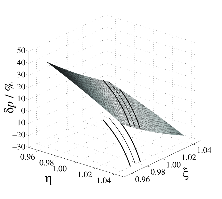
Figure 1: Schnabel et al.

Vapor-liquid equilibria for CO+$\rm C_{2}H_{6}$ were simulated for every combination of
$\eta\in\left[0.96,\,0.98,\,1,\,1.02,\,1.04\right]$ and $\xi\in\left[0.96,\,0.98,\,1,\,1.02,\,1.04\right]$, i.e. overall 25 combinations, using the Grand Equilibrium method [56]. Simulation results of vapor pressure, bubble density and dew point composition are therefore functions of $\eta$ and $\xi$. Their deviations to the experimental values are illustrated as three-dimensional plots in Figures 1 to 3 where the surfaces were derived from the 25 simulation points. All combinations of $\eta$ and $\xi$ which yield the experimental value are plotted as a solid slim line in Figures 1 to 3 and as a projection onto the $\eta$–$\xi$ plane. For the further discussion experimental and simulation uncertainties are needed, where the following estimates were used: 3 % for the vapor pressure, 0.5 % for the bubble density and 4 % (about 0.03 mol/mol) for the dew point composition. These limits are also included in Figures 1 to 3 as solid bold lines.

The vapor pressure significantly dependens on both $\eta$ and $\xi$, cf. Figure 1. It varies by about 35 % for $\eta$ (at constant $\xi$) and 45 % for $\xi$ (at contant $\eta$) in the investigated parameter range. Due to that high sensitivity, the range where the simulated and experimental vapor pressure agree within 3 % is rather small.

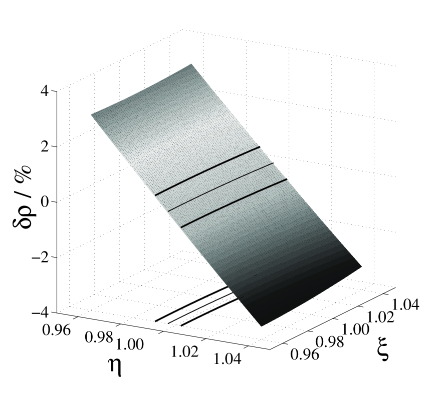
Figure 2: Schnabel et al.

In contrast, the bubble density is practially independent of the parameter $\xi$ as can bee seen from Figure 2, but it varies by about 6 % in the investigated range of $\eta$. The experimental value can be obtained by choosing $\eta$ close to unity in combination with any value of $\xi$ in the regarded range.

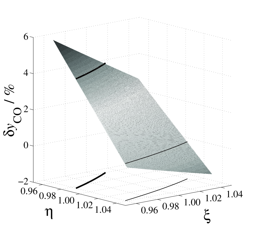
Figure 3: Schnabel et al.

The dew point carbon monoxide mole fraction depends both on $\eta$ and $\xi$ as shown in Figure 3. But it varies only by about 6 % for $\eta$ (at constant $\xi$) and 2 % for $\xi$ (at contant $\eta$) in the investigated parameter range.

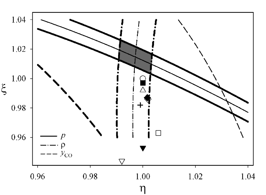
Figure 4: Schnabel et al.

Summarizing Figures 1 to 3 in Figure 4, it can be seen that there is one combination of $\eta$ and $\xi$ where both vapor pressure and bubble density of molecular mixture model and experiment coincide exactly ($\eta=0.9972$ and $\xi=1.0145$). With the uncertainties for the bubble density and the vapor pressure, a target area is defined in which the combination of $\eta$ and $\xi$ yields an accurate description of these both properties, cf. the shaded area in Figure 4. The experimental dew point composition within its (large) uncertainty is also met in this target area.

Figure 4 also allows an easy assessment of the combining rules introduced in Section 2. The LB combining rule is the closest to the target area, but outside of it. All combining rules shown, except SK, describe the bubble density and dew point composition within their assigned uncertainty. However, the experimental vapor pressure is predicted by none of them. The LB combining rule ($\eta=1$ and $\xi=1$) yields deviations from the experimental vapor pressure, bubble density and dew point carbon monoxide mole fraction of $+5.6$ %, $-0.3$ % and $+1.8$ %, respectively. The SK combining rule gives the most remote combination ($\eta=1.0059$ and $\xi=0.9630$) with deviations of $+21.7$ %, $-0.8$ % and $+2.3$ %, respectively.

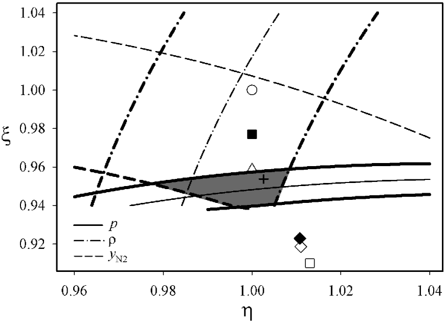
Figure 5: Schnabel et al.

An analogous systematic study for $\rm N_{2}$+$\rm C_{3}H_{6}$ includes 30 vapor-liquid equilibria simulation results for $\eta\in\left[0.96,\,0.98,\,1,\,1.02,\,1.04\right]$ and $\xi\in\left[0.94,0.96,\,0.98,\,1,\,1.02,\,1.04\right]$ at 290 K and $x_{\rm N2}=0.1146$ mol/mol. Since the experimental bubble density was estimated with the Racket model, a higher uncertainty of 1 % was assigned to it. Figure 5 shows the comparison to experimental data where the target area is obtained analogously to the study of CO+$\rm C_{2}H_{6}$. Only the M2 combining rule is within this area, whereas HMC is very close to it. For M2 ($\eta=1.0026$, $\xi=0.9538$) deviations from the experimental vapor pressure, bubble density and dew point nitrogen mole fraction of $-1.7$ %, $-0.8$ % and $+3.0$ % were found, respectively. SK ($\eta=1.013$, $\xi=0.9101$) yields again the most remote results with deviations of $+15.5$ %, $-1.6$ % and $+4.8$ %, respectively.

From both case studies, the conclusion is drawn that the vapor pressure, which significantly depends on both unlike LJ parameters, is the most difficult property to be predicted by combining rules. The bubble density is mainly determined by the unlike LJ size parameter and values close to the arithmetic mean ($\eta=1$) describe the experimental bubble densities well (see also [10, 11]). This is achieved by most of the combining rules. The dew point composition depends on both $\eta$ and $\xi$ like the vapor pressure, however, its sensitivity is considerably weaker compared to the vapor pressure. Due to these findings, it can be recommended to use the Lorentz rule for the size parameter since it predicts bubble densities well and to adjust the unlike energy parameter to the vapor pressure.

4 Comprehensive Study

In previous work [13, 14, 15], molecular models for 44 binary mixtures were developed. For describing the mixture, the Lorentz rule was used for $\sigma_{ab}$, while $\epsilon_{ab}$ was determined using the adjustment parameter $\xi$ as defined by Equation (24). The state independent parameter $\xi$ was optimized by a fit to one experimental vapor pressure data point of the mixture. That procedure chosen in [13, 14, 15] is impressively supported by the results of the case study presented above.

The results from [13, 14, 15] can be directly used to assess combining rules. For combining rules which employ the Lorentz rule for $\sigma_{ab}$ this is completely straight-forward as the adjusted $\xi$ parameter is known and only needs to be compared to the results for the different combining rules. But also combining rules that do not employ the Lorentz rule can be included in the assessment as can be seen from the results of the case study and explained below in more detail.

The pure components of the 44 binary mixtures are of three different molecular model types: spherical and non-polar (1CLJ), anisotropic and dipolar (2CLJD) and anisotropic and quadrupolar (2CLJQ). Hence, six mixture types can be distinguished as given by Table 2. The adjusted unlike LJ energy parameters of those 44 mixture models deviate by up to $\pm 10$ % from the Berthelot rule, cf. Table 3 or see [13, 14, 15].

Seven of the eleven combining rules do not use the Lorentz rule for the unlike LJ size parameter. For an assessment, it has to be investigated by how much they deviate from the Lorentz rule. This was done here with the root mean squares (RMS)

$${\rm RMS}^{\rm x}_{\sigma}=\sqrt{\frac{1}{N}\sum_{i=1}^{N}\left(\eta^{\rm x}-1\right)^{2}}\,,$$ (25)

where $N$ is the number of mixture models to which the particular combining rules (x = H, S, SK, HHG, WH, M1, M2) were applied. In Table 4, ${\rm RMS}^{\rm x}_{\sigma}$ are given distinguishing between the mixture types 1 to 6. It additionally incorporates data taking all 44 binary mixture models into account.

Table 4 shows that the S combining rule yields the same unlike LJ size parameters as the Lorentz rule for all mixture types. Also M2 and SK are very close, deviating by approximately 0.5 % only. The remainder, H, HHG, WH and M1, yield all mean deviations in a narrow band at 1.4 % and below. For mixture type 6, all seven combining rules yield results very close to the arithmetic mean due to fact that all components have very similar parameters. Figures 4 and 5 give an impression of the influence of a variation of $\eta$ of 1 % on the mixture vapor-liquid equilibria. For the pressure and the dew point composition that variation will typically result in changes that do not exceed the experimental uncertainty. For the bubble density the changes are more significant but still the changes do not exceed 1 % in the bubble density. Thus, it can be concluded that there is only a small influence of the combining rules via $\sigma_{ab}$ on the vapor-liquid equilibrium. Therefore, in the following only results of the combining rules for $\xi$ are discussed.

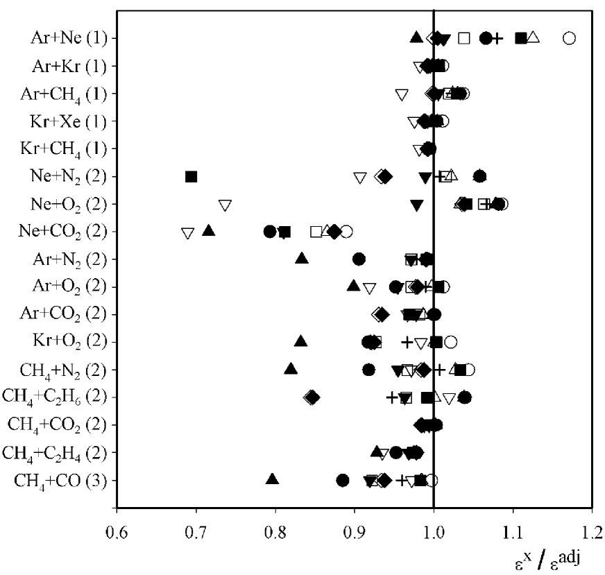
Figure 6: Schnabel et al.

Unlike LJ energy parameters predicted by the eleven combining rules are compared to the adjusted values in Figure 6. The adequacy of the investigated combining rules is indicated by the distance from the reference line (unity), which represents the adjusted LJ energy parameter. Generally, too low dispersion energies are predicted, which is particlularly visible for mixture types 2 to 5. Note that it is implicitly assumed in Figure 6 that the adjusted parameter for $\epsilon_{ab}$ determined in [13, 14, 15] using the Lorentz rule for $\sigma_{ab}$ also holds for the combining rules which apply other approaches for determining $\sigma_{ab}$.

To assess the predictive power of the eleven combining rules the deviations of the unlike LJ energy parameters of the particular combining rules from the adjusted values were summarized by the root mean square

$${\rm RMS}^{\rm x}_{\epsilon}=\sqrt{\frac{1}{N}\sum_{i=1}^{N}\left(\xi^{\rm x}-\xi^{\rm adj}\right)^{2}}\,.$$ (26)

The deviations for all eleven combining rules, distinguishing between mixture types, are given in Table 5. For mixture type 1, for which most of the eleven combining rules were tested, they are better than the LB combining rule. Many of them were fitted to noble gas mixture data and they indeed predict good unlike LJ energy paramters for such mixtures. The reason is that all combining rules, except LB and M2, yield smaller values than the geometric mean. Such a lower unlike dispersion energy is supported by experimental noble gas mixture data [2, 46, 57, 58]. However, for all other mixture types 2 to 5, the combining rules can predict better or worse than the simple LB combining rule. That all combining rules predict similar for mixture type 6 is due to the very similar values of both LJ parameters of the pure components. All in all, the simple LB combining rule has a ${\rm RMS}^{\rm x}_{\epsilon}$ of 5 % which is not significantly worse than those of the best rule (HMC) with 3.9 %, where a variation of $\xi$ by 1 % influences the vapor pressure by about 3 %.

Apart from noble gas mixtures, it can be concluded that none of the inverstigated combining rules has a significant advantage over LB, which yields good bubble densities and vapor compositions, but vapor pressures that deviate from the experiment by an estimated 15 % on average. If highly accurate results for the vapor pressure are needed, an adjustment of the unlike LJ energy parameter to at least one experimental binary vapor pressure data point is necessary in most cases.

5 Conclusion

The dependence of vapor-liquid equilibrium properties on unlike LJ parameters was studied systematically for the mixtures CO+$\rm C_{2}H_{6}$ and $\rm N_{2}$+$\rm C_{3}H_{6}$. This case study shows that the mixture bubble density is accurately obtained using the arithmetic mean of the like LJ size parameters as proposed by the Lorentz combining rule. The bubble density is insensitive to variations of the unlike LJ energy parameter. The vapor pressure is found to be dependent on both unlike LJ parameters. The same is found for vapor phase composition, but with a considerably lower sensitivity. Therefore, it can be recommended to use the Lorentz rule for the unlike LJ size parameter and to adjust the unlike LJ energy parameter to the vapor pressure. Recent investigations on mixtures consisting of more complex molecules, such as ethanol [59, 60], confirm that this procedure holds also in such cases.

Eleven combining rules for unlike LJ parameters, some of which use also other properties than the pure component LJ parameters like ionization potentials or polarizabilities, were investigated regarding their predictive power for vapor-liquid equilibria. They are compared to 44 adjusted mixture models from previous work [13, 14, 15], where the unlike LJ energy parameters were optimized to yield experimental vapor pressure. It is found that the unlike LJ size parameters from the combining rules differ only very litte from the Lorentz rule. Many combining rules investigated here were fitted to noble gas mixture data and they indeed predict good unlike LJ energy paramters for such mixtures. However, none of the investigated combining rules has a significant advantage over LB for other mixture types.

6 Acknowledgment

The authors gratefully acknowledge financial support by Deutsche Forschungsgemeinschaft, Schwerpunktprogramm 1155.

Table 1: Eleven selected combining rules together with the acronyms used here and corresponding references. In the last column, it is indicated whether the unlike LJ size parameter is given by the arithmetic mean, i.e. the Lorentz rule.

Name	Acronym	Reference	Lorentz
Lorentz-Berthelot	LB	[22, 23]	yes
Kohler	K	[26]	yes
Hudson-McCourbrey	HMC	[34]	yes
Fender-Halsey	FH	[38]	yes
Hiza	H	[39, 40, 41]	no
Sikora	S	[42]	no
Smith-Kong	SK	[44, 45]	no
Halgren	HHG	[46]	no
Waldman-Hagler	WH	[47]	no
MATAR-1	M1	[48]	no
MATAR-2	M2	[48]	no

Table 2: Binary mixture types (1–6) classified according to the molecular models of the two components.

	1CLJ	2CLJQ	2CLJD
1CLJ	1	2	3
2CLJQ		4	5
2CLJD			6

Table 3: Unlike LJ energy parameters of the adjusted mixture models taken from [13, 14, 15], grouped according to the mixture type as defined by Table 2.

Mixture		Type	$[\epsilon_{ab}^{\rm adj}/k_{\rm B}]$ / K	Mixture		Type	$[\epsilon_{ab}^{\rm adj}/k_{\rm B}]$ / K
Ne +	Ar	1	053.752	$\rm CO_{2}$ +	$\rm C_{2}H_{6}$	4	128.878
Ar +	Kr	1	136.280	$\rm CO_{2}$ +	$\rm CS_{2}$	4	170.086
Ar +	$\rm CH_{4}$	1	126.974	$\rm CO_{2}$ +	$\rm Cl_{2}$	4	137.020
Kr +	Xe	1	190.225	$\rm C_{2}H_{4}$ +	$\rm C_{2}H_{6}$	4	106.470
Kr +	$\rm CH_{4}$	1	156.184	$\rm C_{2}H_{4}$ +	$\rm C_{2}H_{2}$	4	076.446
Ne +	$\rm N_{2}$	2	032.513	$\rm C_{2}H_{6}$ +	$\rm C_{2}H_{2}$	4	101.267
Ne +	$\rm O_{2}$	2	035.249	$\rm C_{2}H_{4}$ +	$\rm CO_{2}$	4	095.579
Ne +	$\rm CO_{2}$	2	075.559	$\rm C_{2}F_{6}$ +	$\rm CO_{2}$	4	105.045
Ar +	$\rm N_{2}$	2	064.065	$\rm CO_{2}$ +	Propylene	4	130.390
Ar +	$\rm O_{2}$	2	070.164	$\rm C_{2}H_{6}$ +	Propylene	4	146.450
Ar +	$\rm CO_{2}$	2	124.610	$\rm C_{2}H_{4}$ +	Propylene	4	109.654
Kr +	$\rm O_{2}$	2	082.030	$\rm N_{2}$ +	Propylene	4	069.491
$\rm CH_{4}$ +	$\rm N_{2}$	2	068.976	$\rm C_{2}H_{6}$ +	CO	5	072.304
$\rm CH_{4}$ +	$\rm CO_{2}$	2	135.331	$\rm CO_{2}$ +	CO	5	075.719
$\rm CH_{4}$ +	$\rm C_{2}H_{6}$	2	142.225	$\rm N_{2}$ +	CO	5	036.134
$\rm CH_{4}$ +	$\rm C_{2}H_{4}$	2	109.268	$\rm CS_{2}$ +	R22	5	203.132
$\rm CH_{4}$ +	CO	3	074.256	$\rm CO_{2}$ +	R22	5	154.666
$\rm N_{2}$ +	$\rm O_{2}$	4	039.091	$\rm CO_{2}$ +	R23	5	127.914
$\rm N_{2}$ +	$\rm CO_{2}$	4	070.979	R143a +	R134a	6	168.985
$\rm N_{2}$ +	$\rm C_{2}H_{6}$	4	067.344	R125 +	R143a	6	161.770
$\rm N_{2}$ +	$\rm C_{2}H_{4}$	4	049.851	R125 +	R134a	6	168.663
$\rm O_{2}$ +	$\rm CO_{2}$	4	074.255	R143a +	R152a	6	177.304

Table 4: Deviations of the unlike LJ size parameters from the arithmetic mean, i.e. the Lorentz rule, for seven combining rules expressed by the root mean square ${\rm RMS}^{\rm x}_{\sigma}$ as defined by Equation (25) for the different mixture types and for all 44 binary mixture models.

		${\rm RMS}^{\rm x}_{\sigma}$ / %
Combining rule		Mixture type
		1	2	3	4	5	6	all
S, Eq.	(12)	0.0	0.0	0.0	0.0	0.0	0.0	0.0
M2, Eq.	(21)	0.3	0.3	0.2	0.7	0.1	0.0	0.5
SK, Eq.	(13)	0.7	0.6	1.1	0.5	0.3	0.0	0.6
HHG, Eq.	(15)	0.9	1.0	0.7	1.7	0.5	0.0	1.2
H, Eq.	(8)	1.0	1.8	0.3	1.2	0.5	0.1	1.3
WH, Eq.	(17)	1.0	1.2	0.9	2.0	0.7	0.0	1.4
M1, Eq.	(19)	1.0	1.1	0.8	2.0	0.6	0.0	1.4

Table 5: Deviations of the unlike LJ energy parameters from adjusted values for eleven combining rules expressed by the root mean square ${\rm RMS}^{\rm x}_{\epsilon}$ as defined by Equation (26) for the different mixture types and for all 44 binary mixture models. In the last column, it is indicated whether the unlike LJ size parameter is given by the arithmetic mean, i.e. the Lorentz rule.

		${\rm RMS}^{\rm x}_{\epsilon}$ / %
Combining rule		Mixture type							Lorentz
		1	2	3	4	5	6	all
HMC, Eq.	(5)	4.9	04.9	01.6	03.1	04.3	1.4	03.9	yes
M2, Eq.	(22)	3.2	05.2	04.0	03.3	05.3	1.4	04.1	no
SK, Eq.	(14)	0.8	06.1	07.8	02.5	04.7	1.3	04.1	no
S, Eq.	(11)	0.8	07.4	08.1	03.7	04.9	1.4	04.9	no
LB, Eq.	(3)	6.8	05.1	00.3	05.4	03.9	1.4	05.0	yes
K, Eq.	(4)	4.4	11.0	01.7	05.0	04.6	1.5	06.7	yes
M1, Eq.	(20)	0.7	07.2	06.2	08.2	06.7	1.4	06.8	no
WH, Eq.	(18)	0.8	07.4	06.6	08.0	07.0	1.4	06.8	no
HHG, Eq.	(16)	2.9	09.1	11.5	06.8	08.8	1.4	07.3	no
H, Eq.	(9)	2.4	13.6	02.8	07.3	04.8	2.0	08.4	no
FH, Eq.	(7)	1.6	13.9	20.5	10.0	013.3	0.7	11.0	yes

References

- [1] M. Diaz Peña, C. Pando, J.A.R. Renuncio, J. Chem. Phys. 72 (1980) 5269–5275.
- [2] K.T. Tang, J.P. Toennies, Zeitschrift für Physik D 1 (1986) 91–101.
- [3] J. Bzowski, E.A. Mason, J. Kestin, Int. J. Thermophys. 9 (1988) 131–143.
- [4] E.A. Mason, M. Islam, S. Weissmann, Phys. Fluids 7 (1964) 1011–1022.
- [5] R.J. Good, C.J. Hope, J. Chem. Phys. 55 (1964) 111–116.
- [6] M. Diaz Peña, C. Pando, J.A.R. Renuncio, J. Chem. Phys. 76 (1964) 325–332.
- [7] M. Diaz Peña, C. Pando, J.A.R. Renuncio, J. Chem. Phys. 76 (1964) 333–339.
- [8] F. Kohler, J. Fischer, E. Wilhelm, J. Mol. Struct. 84 (1982) 245–250.
- [9] D. Möller, J. Óprzynski, A. Müller, J. Fischer, Mol. Phys. 75 (1992) 363–378.
- [10] J. Vrabec, J. Fischer, Mol. Phys. 85 (1995) 781–792.
- [11] J. Vrabec, J. Fischer. Int. J. Thermophys. 17 (1996) 889–908.
- [12] G. Kronome, I. Szalai, M. Wendland, J. Fischer, J. Mol. Liq. 85 (2000) 237–247.
- [13] J. Stoll, J. Vrabec, H. Hasse, AIChE J. 49 (2000) 2187–2198.
- [14] J. Vrabec, J. Stoll, H. Hasse, Mol. Simul. 31 (2005) 215–221.
- [15] J. Stoll, Molecular Models for the Prediction of Thermophysical Properties of Pure Fluids and Mixtures, Fortschritt-Berichte VDI, Reihe 3, 836, VDI Verlag, Düsseldorf 2004.
- [16] J. Vrabec, J. Stoll, H. Hasse, J. Phys. Chem. B 105 (2001) 12126–12133.
- [17] J. Stoll, J. Vrabec, H. Hasse, J. Chem. Phys. 119 (2003) 11396–11407.
- [18] J. Vrabec, G.K. Kedia, H. Hasse, Cryogenics 45 (2005) 253–258.
- [19] G.A. Fernández, J. Vrabec and H. Hasse, Int. J. Thermophys. 25 (2004) 175–186.
- [20] G.A. Fernández, J. Vrabec, H. Hasse, Fluid Phase Equilib. 221 (2004) 157–163.
- [21] J. Vrabec, J. Fischer, AIChE J. 43 (1997) 212–217.
- [22] H.A. Lorentz, Annalen der Physik 12 (1881) 127–136.
- [23] D. Berthelot, Comptes Rendus de l’Académie des Sciences Paris 126 (1889) 1703–1706.
- [24] J. Delhommelle, P. Millié, Mol. Phys. 99 (2001) 619–625.
- [25] P. Ungerer, A. Wender, G. Demoulin, E. Bourasseau, P. Mougin, Mol. Simul. 30 (2004) 631–648.
- [26] F. Kohler, Monatsh. Chem. 88 (1957) 857–877.
- [27] F. London, Z. Phys. Chem. (Leipzig, Ger.) 11 (1930) 222–251.
- [28] F. London, Transactions of the Faraday Society 33 (1937) 8–26.
- [29] K.E. Laidig, R.F.W. Bader, J. Chem. Phys. 93 (1990) 7213–7224.
- [30] R.D. Lide, CRC Handbook of Chemistry and Physics, 76th ed., CRC Press Inc., New York, 1995-1996.
- [31] C. D. Wood, K. Senoo, C. Martin, J. Cuellar and A.I. Cooper, Macromolecules 35 (2002) 6743–6746.
- [32] M. Fermeglia, M. Ferrone, S. Pricl, Fluid Phase Equilib. 210 (2003) 105–116.
- [33] O. Echt, D. Kreisle, E. Recknagel, J.J. Saenz, R. Casero and J.M. Soler, Phys. Rev. A 38 (1988) 3236–3248.
- [34] G.H. Hudson, J.C. McCoubrey, Transactions of the Faraday Society 56 (1960) 761–766.
- [35] T.M. Reed, III, J. Phys. Chem. 59 (1955) 425–428.
- [36] B.N. Srivastava, M.P. Madan, Proceedings of the Physical Society of London Section A 66 (1953) 278–287.
- [37] R.C. Reid, T.W. Leland, AIChE J. 11 (1965) 228–237.
- [38] B.E.F. Fender and G.D. Halsey, J. Chem. Phys. 36 (1962) 1881–1888.
- [39] M.J. Hiza, A.G. Duncan, Phys. Fluids 12 (1969) 1531–1532.
- [40] M.J. Hiza, A.G. Duncan, AIChE J. 16 (1970) 733–738.
- [41] M.J. Hiza, R.L. Robinson, J. Chem. Phys. 68 (1978) 4768–4769.
- [42] P.T. Sikora, J. Phys. B 3 (1970) 1475–1482.
- [43] G.C. Maitland, Intermolecular Forces, Clarendon Press, Oxford, 1981.
- [44] F.T. Smith, Phys. Rev. A 5 (1972) 1708–1713.
- [45] C.L. Kong, J. Chem. Phys. 59 (1973) 2464–2467.
- [46] T.A. Halgren, J. Am. Chem. Soc. 114 (1992) 7827–7843.
- [47] M. Waldman, A.T. Hagler, J. Comput. Chem. 14 (1993) 1077–1084.
- [48] A.K. Al-Matar, D.A. Rockstraw, J. Comput. Chem. 25 (2004) 660–668.
- [49] D.B. Trust and F. Kurata, AIChE J. 17 (1971) 415–419.
- [50] D.B. Robinson, D.-Y. Peng, S.Y.-K. Chung, Fluid Phase Equilib. 24 (1985) 25–41.
- [51] J.F. Ely, J.W. Magee, W.M. Haynes, NBS standard reference database 14, DDMIX, Version 9.06. NIST, Boulder, Colorado 1989.
- [52] L. Grausø, A. Fredenslund, J. Mollerup, Fluid Phase Equilib. 1 (1977) 13–26.
- [53] H.G. Rackett, Journal of Chemical and Engineering Data 15 (1970) 514–517.
- [54] C.F. Spencer, R.P. Danner, Journal of Chemical and Engineering Data 18 (1973) 230–234.
- [55] P.L. Chueh, J.M. Prausnitz, AIChE J. 13 (1967) 1099–1107.
- [56] J. Vrabec, H. Hasse, Mol. Phys. 100 (2002) 3375–3383.
- [57] J. Kestin, K. Knierim, E.A. Mason, B. Najafi, S.T. Ro, M. Waldman, J. Phys. Chem. Ref. Data 13 (1984) 229–303.
- [58] J. Bzowski, J. Kestin, E.A. Mason, F.J. Uribe, J. Phys. Chem. Ref. Data 19 (1990) 1179–1232.
- [59] T. Schnabel, J. Vrabec, H. Hasse, Fluid Phase Equilib. 233 (2005) 134–143.
- [60] T. Schnabel, J. Vrabec, H. Hasse, Fluid Phase Equilib. 239 (2006) 125–126.