Stochastic dynamics of phase-slip trains and superconductive-resistive switching in current-biased nanowires

Abstract

Superconducting nanowires fabricated via carbon-nanotube-templating can be used to realize and study quasi-one-dimensional superconductors. However, measurement of the linear resistance of these nanowires have been inconclusive in determining the low-temperature behavior of phase-slip fluctuations, both quantal and thermal. Thus, we are motivated to study the nonlinear current-voltage characteristics in current-biased nanowires and the stochastic dynamics of superconductive-resistive switching, as a way of probing phase-slip events. In particular, we address the question: Can a single phase-slip event occurring somewhere along the wire—during which the order-parameter fluctuates to zero—induce switching, via the local heating it causes? We explore this and related issues by constructing a stochastic model for the time-evolution of the temperature in a nanowire whose ends are maintained at a fixed temperature. We derive the corresponding master equation as tool for evaluating and analyzing the mean switching time at a given value of current (smaller than the de-pairing critical current). The model indicates that although, in general, several phase-slip events are necessary to induce switching via a thermal runaway, there is indeed a regime of temperatures and currents in which a single event is sufficient. We carry out a detailed comparison of the results of the model with experimental measurements of the distribution of switching currents, and provide an explanation for the rather counter-intuitive broadening of the distribution width that is observed upon lowering the temperature. Moreover, we identify a regime in which the experiments are probing individual phase-slip events, and thus offer a way of unearthing and exploring the physics of nanoscale quantum tunneling of the one-dimensional collective quantum field associated with the superconducting order parameter.

I Introduction

The fundamental process governing the collective physical properties of quasi-one-dimensional superconducting systems is the phase-slip process exhibited by the extended, complex-valued superconducting order parameter field $\Psi(z)$, which depends on the position $z$ along the system. In the course of a phase-slip process, the field $\Psi(z)$, undergoes a transition from an initial (typically metastable) supercurrent-carrying state $\Psi_{1}(z)$ to a final one $\Psi_{2}(z)$. In settings in which the voltage drop between the ends of the system is externally controlled, these metastable states are topologically distinct from one another: the total changes, $\int dz\,d\Phi_{j}(z)/dz$, in their position-dependent phases $\Phi_{j}(z)$, from one end of the system to the other, differ by $2\pi$, and the supercurrents carried by these states differ, too FN:setting .

In the absence of phase-slip processes, the order parameter field of quasi-one-dimensional superconducting systems behaves reversibly, i.e., energy stored as kinetic energy associated with supercurrent remains undissipated. If, however, phase-slip processes do occur, so can dissipation, part of the coherent kinetic energy of superflow being converted into incoherent motion, i.e., heat. For example, in a voltage-controlled setting, current-reducing phase slips occur with a higher frequency than current-increasing ones, leading to energy and current dissipation and the notion of an intrinsic resistance, as elucidated by Little Little1967 and Langer and Ambegaokar LangerA1967 . Similarly, in a current-controlled setting McCumber1968 , the preferred sense of phase-slip processes yields an average voltage consistent with a positive Joule-heating power. This is the sense in which phase-slip processes control the collective properties of quasi-one-dimensional superconducting systems: they constitute the building blocks via which one can understand properties such as dissipation.

In principle, transitions in the state of the order-parameter field can behave predominantly either classically or quantally, depending on the temperature of the system. In the classical regime, being metastable, the states are local minima of the classical free energy, and the transitions between such states constitute thermal fluctuations of the order-parameter field over the Arrhenius energy barriers that separate these states. The study of the rates at which such transitions occur, and their implications for collective charge-transport through superconducting nanowires, was initiated by Little Little1967 , and developed in detail, shortly thereafter, by Langer and Ambegaokar LangerA1967 and McCumber and Halperin McCumberH1970 . In the quantal regime, the transitions between the states are quantum tunneling events, in which the entire, extended, order-parameter field passes from one metastable state to another through a classically forbidden region of field configurations GrabertW1984 ; Giordano1990 .

In this Paper we develop a theory of the kinetics of phase slips of the superconducting order-parameter field in settings in which the heat liberated or absorbed during these processes is not instantaneously dissipated but, rather, leads to alterations in the local temperature of the quasi-one-dimensional system and a resulting flow of heat, which feed back to influence the phase-slip kinetics. As discussed by Tinkham and co-workers TinkhamFLM2003 , this feedback leads to a switching bistability of the system involving a pair of mesoscopic states: an essentially superconducting, low-voltage state and a more highly resistive, high-voltage state. The rarity of phase slips in the essentially superconducting state mean that very little Joule heating takes place, which favors the persistence of this state. However, the energy liberated by concentrated bursts of phase slips can Joule-heat the system enough to weaken the superconductivity, which enhances the likelihood of phase slips, and—via this feedback loop—lead to the essential destruction of the superconductivity and the maintenance of the more strongly Joule-heated, more highly resistive state.

Recent advances in sample preparation techniques have made possible the fabrication and exploration of extraordinarily narrow nanowires. These wires can be so fine, say $10\,\text{nm}$ wide or even less, that they bring within reach experimental conditions in which heat liberated during small numbers of phase-slip events—and perhaps even a single one—can have a dramatic impact on the state of the wire, triggering the switching transition from the superconducting to the resistive state. Thus, by monitoring the voltage between the ends of the wire one should be able to observe macroscopic, or at least mesoscopic, consequences of an individual phase slip, and hence investigate the properties of these nanoscale building-blocks of the collective behavior of quasi-one-dimensional superconductivity. For example, one should be able to ascertain the rate at which phase slips occur, and its dependence on temperature, applied current, wire geometry and materials parameters. One should also be able to compare such rates with those suggested by theoretical pictures in which the phase slips proceed primarily via thermal activation over an energy barrier or via quantum tunneling through one. Hence, one should be able to move beyond the nanoscience that observes the structure of nanomaterials or single-particle phenomena within them, and progress towards a nanoscience of collective processes.

The theory developed in this Paper aims to take a step beyond Ref. TinkhamFLM2003 by considering the stochastic aspects of the phase-slip processes occurring in quasi-one-dimensional superconducting systems, i.e., by allowing for sequences of phase-slips that occur at random intervals of time, and exploring the consequences of this stochasticity for the states exhibited by the system. Our main focus will be on the implications of this underlying stochasticity for the rate at which quasi-one-dimensional superconducting systems undergo switching transitions from the essentially superconducting state to the more highly resistive state, as a function of the temperature and the current at which the system is maintained. Experiments are commonly done in a mode in which the current is not maintained at a fixed value but is, rather, repeatedly ramped up at some fixed rate of increase, the current at which the switching transition occurs being monitored, so as to produce a distribution of switching currents, which depends on the temperature and the ramping rate of the current Sahu2008 ; Sahu2008b .

Motivation for work reported in this Paper comes from the kinds of experimental investigations of superconductivity in nanowires touched upon in the previous paragraph, and the concomitant need for a road map to guide experimental investigations towards regimes of current and temperature in which small numbers of phase-slip events, or even single such events, induce switching transitions of essentially superconducting wires to a highly resistive state. Experiments performed in this regime should provide access to the temperature- and current-dependence of the rate at which individual phase-slip events occur. A brief account of this work was reported in Ref. Shah2008 .

The Paper is structured as follows: In Sec. II we describe the switching-current experiments on hysteretic superconducting nanowires along with details of our physical picture of superconducting-resistive switching. We construct a stochastic model of the dynamics of the temperature in superconducting nanowires wires in Sec. III, and explore its basic properties in Sec. IV. Next, we develop a formalism to address the the statistics of switching events in Sec. V, and use it to compute the switching rate as a function of temperature and bias current in Sec. VI, and, in turn, compare this rate to experiments in Sec. VII. Finally, we present some concluding remarks in Sec. VIII.

II Physical scenario for switching in current-biased nanowires

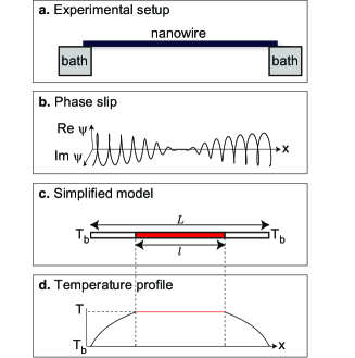
Figure 1: Schematic showing a. the configuration of the free-standing nanowire supported by the superconducting leads, which act as a thermal bath; b. the attenuation of the order parameter $\psi(x)$ in the core of a phase slip; c. the simplified model of the wire: phase-slips occur exclusively in the central segment while the end segments carry the heat produced by phase-slips to the thermal baths; d. the temperature profile of the wire in the simplified model, with uniform temperature in the central segment and spatially varying temperature in the end segments.

The ultranarrow wires that we consider in this Paper were fabricated using molecular templating BezryadinLT2000 ; HopkinsPGB2005 . By using a solution containing long molecules such as carbon nanotubes or DNA one can create a configuration in which a nanotube traverses a trench, so as to form a bridge-like structure. One can then deposit a layer of superconductor, such as MoGe or Nb, on top so that the nanotube provides scaffolding on which to form a superconducting nanostructure. In effect, one can thus fabricate a set-up in which a free-standing superconducting nanowire is connected at both of its ends to superconducting leads, as shown in Fig. 1a. The diameter of the resulting nanowire can be made smaller than the coherence length of the superconductor, and the length of the wire sufficiently greater than the coherence length so that the nanowire provides a realization of a quasi-one dimensional superconductor in which the superconducting fluctuations are effectively one dimensional. Through careful control, the wires produced via molecular templating can be made amorphous and quite homogeneous. The resulting superconductor ends up being in the dirty limit (i.e., the electron mean-free-path is smaller than both the coherence length and the penetration depth).

Upon lowering the temperature, the resistance of the nanostructure (i.e., the leads and the nanowire) exhibits two drops: a sharp drop as the leads become superconducting, and a second, much smoother transition, corresponding to the onset of superconductivity in the nanowire itself. The broad resistive transition of the nanowire can be understood in terms of the occurrence of thermally activated phase-slip fluctuations, and can be quantitatively fit in terms of the Langer-Ambegaokar-McCumber-Halperin (LAMH) theory LangerA1967 ; McCumber1968 ; McCumberH1970 by using the transition temperature and the coherence length as fitting parameters. However, the behavior of the resistance at very low temperatures is not unambiguously established, either theoretically or experimentally. On the one hand, time-dependent Ginzburg-Landau theory, which forms the basis of the LAMH calculation, is not strictly applicable in this regime of temperatures and, in addition, phase slip processes involving quantum tunneling rather than thermal barrier crossing are expected to become important in this regime. And on the other hand, the value of the resistance can fall below the noise floor of the experiment.

To overcome the difficulty in probing superconductivity in nanowires at low temperatures associated with the smallness of the linear resistance, we focus on experiments involving high bias-currents so that they lie beyond the linear-response regime. In these experiments, the current through the nanowire is ramped up and down in time, via a triangular or sinusoidal modulation protocol. As the current is ramped up, the state of the wire switches from superconductive to resistive (i.e., normal), doing so at a value of the current that is smaller than the de-pairing (i.e., equilibrium) critical current; and on ramping the current down, the state gets re-trapped into a superconductive state, but at a value of current smaller than the current at which switching occurred. Hysteretic behavior such as this, reflecting the underlying bistability of the superconducting nanowire over a temperature-dependent interval of currents, was first reported in Ref. TinkhamFLM2003 . The experiments addressed in the present paper Sahu2008 ; Sahu2008b go a step further, in that they repeatedly ramp the current up and then down, for thousands of cycles at each of a chosen set of temperatures, and thus generate thousands of values of the switching and re-trapping currents at each of these temperatures. These experiments find that the distribution of re-trapping currents is very narrow and does not significantly change with temperature. In contrast, the distribution of switching currents is relatively broad, the mean and the width of the distribution changing as the bath temperature—which is set by the leads—is varied. The fact that even at a fixed temperature and current-sweep protocol the switching current is statistically distributed and does not have a sharp value is a reflection of (and therefore a window on) the collective dynamics of the superconducting condensate in the nanowire. The condensate is seen to be a fluctuating entity, evolving stochastically in time and, at random instants, undergoing phase slip events. The goal of the present work is to understand the behavior of these distributions of switching currents, and thereby gain insight into the low-temperature rates at which thermal and quantum phase-slip fluctuations occur. We now proceed to motivate the physical mechanism for switching, and thus set the stage for the remainder of this Paper.

Distributions of switching currents were first studied in the context of Josephson junctions, in work by by Fulton and Dunkleberger FultonD1974 . In particular, these researchers found that the width of the distribution decreased, as the temperature was reduced. As will be discussed in detail in Sec. VII, in the experiments on nanowires that we are considering Sahu2008 ; Sahu2008b , this width is found to increase as the temperature is reduced. A second important difference is that the Josephson junctions that show hysteresis are under-damped systems, whereas nanowires are expected to be over-damped, as argued also in Ref. TinkhamFLM2003 , i.e., a single phase-slip event by itself is sufficient to cause switching in hysteretic Josephson junctions but not in superconducting nanowires. Experimentally, the observation of voltage tails Rogachev ; AltomareCMHT2006 ; Sahu2008b , i.e., small but non-zero voltages across current-biased nanowires in the superconducting state, verifies the occurrence of multiple phase slips prior to the switching event, and indicates that the wire is in the over-damped regime. The main consequence of these arguments is that while in the experiments reported by Fulton and Dunkleberger the rate of switching is essentially given by the rate $\Gamma$ at which individual phase-slips occur, in the case of nanowires the switching rate is generically found to be smaller than $\Gamma$. Tinkham and co-workers TinkhamFLM2003 have proposed a physical mechanism that accounts for the fact that hysteresis in observed, in spite of the over-damped dynamics of the wire. According to this mechanism, the phase-slip fluctuations are resistive but, because of the over-damping, they are not by themselves capable of causing switching to a resistive (i.e., normal) state. However, the resistance coming from the phase-slip fluctuations is associated with Joule heating. If this heating is not overcome sufficiently rapidly (e.g., by conductive cooling) then it has the effect of reducing the de-pairing current, ultimately to below the applied current, thus causing switching to the highly resistive state. Given that the wire is free-standing, heat can leave the wire only by conducting it to the bath provided by the leads to which each of its ends is connected. In the following sections, we discuss in more detail how bistability and hysteresis come about within the framework of this physical picture. Along the way, it should become clear how, within this picture, switching induced by multiple phase-slips can essentially be interpreted in terms of the number of phase-slips needed to cause a kind of thermal runaway instability of the superconducting state.

III Building a Model for Heating By Phase Slips

The goal of this section is to construct a theoretical model of the stochastic dynamics that leads to the switching of current-biased nanowires from the superconductive to the resistive state. We begin by reviewing the theory of the steady-state thermal hysteresis as set out in Ref. TinkhamFLM2003 . We continue by replacing the steady-state heating of the wire by heating via discrete stochastic phase-slips. The main result of this section is a Langevin-type stochastic differential equation that describes the dynamics of the temperature within the wire.

III.1 Thermal hysteresis mechanism

The thermal mechanism for hysteresis in superconducting nanowires was originally proposed by Tinkham et al. TinkhamFLM2003 . The qualitative idea of this mechanism, along with its relevance to experiments on superconducting nanowires, was discussed in the previous section. In the present subsection we set up the quantitative description of the mechanism by giving a brief account of their work, and thus set the stage for our stochastic extension of it. Their description rests on the premise that the temperature of the wire is controlled by a competition between (i) Joule heating, and (ii) cooling via the conduction of heat to the baths (leads). If ${\Theta}(x)$ is the temperature at position $x$ along the wire of length $L$ and cross-sectional area $A$, then the power-per unit length dissipated due to Joule heating at a bias current $I$ is taken to be

$$Q_{\text{source}}(x)=\frac{I^{2}R\big{(}{\Theta}(x),I\big{)}}{AL},$$ (1)

where the function $R({\Theta}^{\prime})$ is to be understood as the resistance of an entire wire held at a uniform temperature ${\Theta}(x)={\Theta}^{\prime}$. On the other hand, as the wire is suspended in vacuum, the heat is almost exclusively dissipated through its conduction from the wire to the superconducting leads that are held at a temperature $T_{b}$ and which play the role of thermal bath. The heating and cooling of the wire is described by the corresponding static heat conduction equation:

$$Q_{\text{source}}(x) =-\partial_{x}\left[K_{\text{s}}({\Theta})\,\partial_{x}{\Theta}(x)\right]$$ (2)

$$=-\frac{\partial K_{s}(\Theta)}{\partial\Theta}\left(\partial_{x}\Theta\right)^{2}-K_{s}(\Theta)\partial_{x}^{2}\Theta,$$ (3)

where $K_{\text{s}}({\Theta})$ is the thermal conductivity of the wire (The first term on the right-hand side of Eq. (3) was absent in Ref. TinkhamFLM2003 ). This equation is supplemented by the boundary conditions ${\Theta}(\pm L/2)=T_{\text{b}}$ at the wire ends, $x=\pm L/2$, and we solve it numerically via the corresponding discretized difference equation.

It was found in Ref. TinkhamFLM2003 that Eq. (3) yields two solutions for a certain range of $I\$and $T_{\text{b}}$. The nonlinear dependence of the resistance $R$ on temperature, which is characteristic of a superconducting nanowire, is at the root of this bistability. This bistability in turn furnishes the mechanism for the thermal hysteresis in the $I$–$V$ characteristic; the two solutions correspond to the superconducting (cold solution) and the resistive (hot solution) branches of the hysteresis loop. To obtain the hysteresis loop at a given bath temperature $T_{\text{b}}$, one begins by solving Eq. (2) to obtain ${\Theta}(x)$ at a bias current sufficiently low such that the equation yields only one solution. Next, by using the solution ${\Theta}(x)$ from the previous step to initialize the equation solver for the next bias current step, the locally stable solution of Eq. (2) is traced out as a function of $I$ by tuning the bias current first up and then down. The $I$–$V$ loop is thus traced out by calculating the voltage,

$$V=\int_{-L/2}^{L/2}dx\,IR\big{(}{\Theta}(x),I\big{)},$$ (4)

at each step.

The numerical analysis of Eq. (2) requires a knowledge of $R\big{(}\Theta,I\big{)}$ and $K_{\text{s}}\big{(}\Theta\big{)}$, which serve as input functions for the theory. A discussion of these input functions and other parameters is given in Appendix A. In Ref. TinkhamFLM2003 , the linear-response resistance measured at $T_{\text{b}}=\Theta$ was used for $R(\Theta,I)$. However, $R(\Theta,I)$ depends also on the value of the bias current $I$. Moreover, we find that by incorporating deviations in $R(\Theta,I)$ from the linear-response regime, we are also able to obtain a better fit with the experiments considered in this Paper (see Ref. Sahu2008b and Appendix A).

III.2 Heating by discrete phase slip events: Derivation of Langevin equation

In the previous subsection, we described the static theory of thermal hysteresis as was discussed in Ref. TinkhamFLM2003 in the context of experiments on MoGe nanowires. Let us now go one step further and include dynamics by considering the time-dependent heat diffusion equation:

$$C_{\text{v}}({\Theta})\,\partial_{t}{\Theta}(x,t)=\partial_{x}\left[K_{\text{s}}({\Theta})\,\partial_{x}{\Theta}(x,t)\right]+Q_{\text{source}},$$ (5)

where the specific heat $C_{\text{v}}({\Theta})$ enters as an additional input function. This differential equation can be derived in the standard way, by using the continuity equation,

$$\nabla\cdot j_{Q}+\partial_{t}Q=Q_{\text{source}}$$ (6)

for the heat current,

$$j_{Q}\equiv-K_{s}(\Theta)\nabla\Theta,$$ (7)

together with the energy density,

$$Q\equiv\int^{\Theta(x)}C_{v}(\Theta^{\prime})d\Theta^{\prime}.$$ (8)

However, as long as we assume that the wire is heated by the source term given by Eq. (1), the dynamic formulation turns out to be inadequate for our purposes, as should become clear from our analysis and results. Such a source term assumes that the wire is being continually heated locally as a result of its resistivity $R({\Theta}(x),I)A/L$ at any given position $x$ along the wire. Is this assumption of continual Joule heating correct? To answer this question we need to deconstruct the resistance and get to its root. In Sec. II we have dwelt upon phase-slip fluctuations in detail. There, we have emphasized the essential point that it is the resistive phase-slip fluctuations that are responsible for the characteristic resistance of a quasi-one dimensional wire. Thus, one should consider the Joule heating as being caused by individual, discrete phase-slip events.

Let us then explicitly consider discrete phase-slip events (labeled by $i$) that take place one at a time at random instants of time $t_{i}$, and are centered at random spatial locations $x_{i}$. By using the Josephson relation

$$\frac{d\phi}{dt}=\frac{2eV}{\hslash}=\frac{2\pi V}{\Phi_{0}},$$ (9)

relating the voltage pulse $V(t)$ to the rate of change of the end-to-end phase difference across the wire $\phi$, we arrive at the work done on the wire by a phase slip, viz.,

$$W_{\text{ps}}=\int dt\,IV=I\int_{0}^{2\pi}d\phi\,\frac{\hbar}{2e}=\Phi_{0}I,$$ (10)

where $\Phi_{0}=h/2e$ is the superconducting flux quantum. Hence, a single phase slip (or anti-phase slip), which corresponds to a decrease (or increase) of $\phi$ by $2\pi$, will heat (or cool) the wire by a “quantum” of energy $W_{\text{ps}}$. By using this result we can now write down a time-dependent stochastic source term:

$$Q_{\text{source}}(x,t)\equiv\frac{W_{\text{ps}}}{A}\sum_{i}\sigma_{i}\,F(x-x_{i})\,\delta(t-t_{i}),$$ (11)

where $F(x-x_{i})$ is a spatial form factor, of unit weight, representing the relative spatial distribution of heat produced by the $i^{\text{th}}$ phase-slip event, and $\sigma_{i}=\pm 1$ for phase (anti-phase) slips. The probability per unit time $\Gamma_{\pm}$ for anti-phase (phase) slips to take place depends on the local temperature ${\Theta}(x,t)$ and the current $I$.

Now, instead of using the continual Joule-heating source term, Eq. (1), let us use the source term given by Eq. (11). Instead of being a deterministic differential equation, the heat diffusion equation (5) becomes a stochastic differential equation for $T(x,t)$. We thus have a Langevin equation with stochasticity, in one space and one time dimension, with a “noise” term that is characteristic of a jump process.

Let us pause to understand the connection between the two source terms. By using the Josephson relation (9), we can express the resistance as

$$R(\Theta,I)=\frac{V}{I}=\frac{1}{I}\frac{\Phi_{0}}{2\pi}\frac{d\phi}{dt}=\frac{\Phi_{0}\,\Gamma(\Theta,I)}{I},$$ (12)

and use it to rewrite the continual Joule-heating source term, Eq. (1), as

$$Q_{\text{source}}=\frac{W_{\text{ps}}\,\Gamma(\Theta,I)}{A\,L},$$ (13)

where $\Gamma\equiv\Gamma_{-}-\Gamma_{+}$ is the net phase-slip rate for the entire wire. Let us assume that a phase slip only affects its local neighborhood, i.e., $F(x-x_{i})\sim\delta(x-x_{i})$. Then, if we take the continuous time limit of Eq. (11) by assuming that the phase-slips are very frequent and that $Q_{\text{ps}}\rightarrow 0$, the two source terms would indeed become equivalent (as can also be seen formally by taking the limit $\Phi_{0}\rightarrow 0$).

We now make a brief remark about the switching current. The static theory of hysteresis that was discussed in the previous subsection has a single, well-defined value of the switching current, which corresponds to the value of the bias current at which the low-temperature (superconductive) solution becomes unstable. On the other hand, we see from the theory discussed in the present subsection that the randomness in $x_{i}$ and $t_{i}$ generates a stochasticity in the switching process. The full implications of the stochastic dynamical theory will be discussed in the following sections.

III.3 Simplified model: Reduced Langevin equation

In principle, one can proceed to study the physics of the stochastic switching dynamics of a current-biased nanowire by using the dynamics of Eq. (5) together with stochastic source Eq. (11), both derived in the previous subsection. In practice, however, it is not easy to solve the full Langevin equation with both spatial and temporal randomness. In this subsection we derive a simplified model, and argue that it is capable of capturing the physics essential for our purposes.

We concentrate on wires that are in the dirty limit, for which the mean free path is much shorter than the coherence length, which is shorter than the charge imbalance length required for carrier thermalization, which itself is somewhat shorter than the nanowire length $L$. In addition to restrictions on length-scales, we assume that the time for a phase-slip ($\sim\tau_{\text{GL}}$) and the quasi-particle thermalization time $\tau_{\text{E}}$ are both smaller than the wire cooling time, i.e., the time it takes the heat deposited in the middle of the wire by a phase-slip to diffuse out of the wire.

We will make a series of simplifications as follows:

1. Due to the presence of the superconducting leads at two ends, as well as edge effects, it is more likely that the phase-slip fluctuations in the wire are centered away from the wire edges. We thus assume that the source term is restricted to a region near the center of the wire.

2. We assume that the heating takes place within a central segment of length $l$, to which a uniform temperature $T$ is assigned. Note that the total length $L$ may be allowed to differ slightly from the geometric length of the wire, in order to compensate for the temperature gradients in the lead at the wire attachment points.

3. We assume that heat is conducted away through the end segments, each of which are of length ($L-l)/2$. As an additional simplification, we ignore the heat capacity of these end segments.

4. To simplify the problem further, we make use of the fact that the probability per unit time (i.e., the characteristic rate) $\Gamma_{+}$ for an anti-phase slip to take place is much smaller than the rate $\Gamma_{-}$ for a phase slip to take place, and we thus ignore the process of cooling by anti-phase slips. To account indirectly for their presence, we use a reduced rate $\Gamma\equiv\Gamma_{-}-\Gamma_{+}$ instead of $\Gamma_{-}$. This ensures that the discrete expression for $Q$ correctly reduces to the continual Joule-heating expression.

With the simplified model defined above, the description of superconducting nanowires reduces to a stochastic ordinary differential equation for the time-evolution of the temperature $T$ of the central segment:

$$\frac{dT}{dt}=-\alpha(T,T_{\text{b}})(T-T_{\text{b}})+\eta(T,I)\sum_{i}\delta(t-t_{i}).$$ (14)

This equation can be regarded as a spatially reduced Langevin-type equation which is a counterpart to the full, spatially dependent Langevin-type equation (5) and, correspondingly, has a spatially reduced version of the full source term (11). The second term on the RHS of Eq. (14) corresponds to (stochastic) heating by phase slips, and the first to (deterministic) cooling as a result of the conduction of heat from the central segment to the external bath via the two end-segments. The temperature-dependent cooling rate $\alpha(T,T_{\text{b}})$ is obtained by comparing the heat currents through the end segments to the thermal mass of the central segment, where the heat currents through the end segments are found by solving the heat equation in the end segments, subject to the boundary conditions that $T(0)=T(L)=T_{\text{b}}$ and $T(\frac{L-l}{2})=T(L-\frac{L-l}{2})=T$. The cooling rate may be expressed in terms of the integral

$$\alpha(T,T_{\text{b}})\equiv\frac{4}{l(L-l)C_{\text{v}}(T)}\frac{1}{T-T_{\text{b}}}\int_{T_{\text{b}}}^{T}dT^{\prime}\,K_{\text{s}}(T^{\prime}).$$ (15)

If $T_{\text{i}}$ and $T_{\text{f}}$ are temperatures of the central segment before and after a phase slip then we can express the temperature ‘impulse’ due to a phase slip, i.e., $T_{\text{f}}-T_{\text{i}}\equiv\eta(T_{\text{i}},I)\equiv\widetilde{\eta}(T_{\text{f}},I)$, as function of either $T_{\text{i}}$ or $T_{\text{f}}$ (depending on the context) by using

$$A\text{ }l\int_{T_{\text{i}}}^{T_{\text{f}}}C_{\text{v}}(T^{\prime})\,dT^{\prime}=Q_{\text{ps}}.$$ (16)

To summarize, in this section we have derived a simplified model that is described by the reduced Langevin equation (14). The central assumption that we used to build this simplified model is that phase-slips predominantly occur in the center of the nanowire, or at least that their exact spatial locations are unimportant. This assumption is appropriate for shorter nanowires, in which we do not have several distinct locations along the wire at which a switching event may nucleate. Specifically, if the wire length does not greatly exceed the charge imbalance length (which itself is assumed to be much larger than the coherence length) then, independent of where a phase-slip occurs, the temperature profile in the wire after the phase slip will be similar, and we are able to apply our simplified time-only model.

IV Basic properties of the Simplified Model: Bistability and switching

The goal of this section is to explain the basic properties of the stochastic model that was formulated in the previous section and is described by the reduced Langevin equation, Eq. (14). First, we show explicitly that the competition between the heating and cooling terms leads to the emergence of bistability. Next, we show that the stochastic character of the heating term can lead to switching between the two metastable states. Then, to characterize this switching we relate the lifetime of the superconducting state to the Mean First Passage Time (MFPT) for the temperature $T$ in the central segment to exceed a certain critical value $T^{\ast}$.

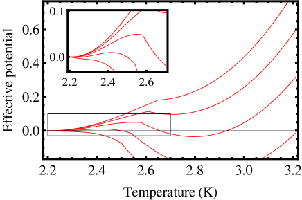
Figure 2: Effective potentials for various bias currents ($0.175$, $0.195$, $0.215$, $0.235$, $0.255\,\mu\text{A}$) at fixed lead temperature $T_{\text{b}}=1.2\,\text{K}$ FN:parameters . The inset shows the details of the local maximum of the effective potential, and corresponds to an enlargement of the region indicated by the box in the main plot.

We begin by reminding the reader that the theory of Ref. TinkhamFLM2003 , described by Eq. (3) with the source term given by Eq. (1), is the static continual-heating version of the theory described by Eq. (5) with the source term given by Eq. (11). The connection is made evident via Eq. (13). As has been shown at the end of Subsection III.1, for certain values of $T_{\text{b}}$ and $I$ the continual-heating theory describes a bistable system having a low-temperature superconducting branch and a high-temperature resistive branch. The fluctuating theory described by Eqs. (5) and (11), in turn, allows for processes that move the system between the two metastable states.

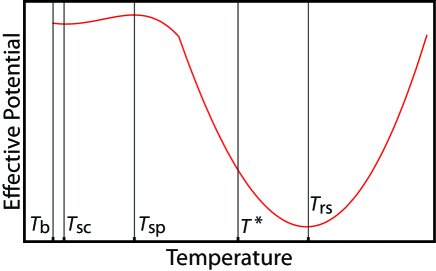
Figure 3: Schematic depiction of the effective potential for the bistable case, showing the labeling scheme for the various temperatures: the bath temperature $T_{\text{b}}$, effective-potential minima corresponding to the superconducting state $T_{\text{sc}}$ and the resistive state $T_{\text{rs}}$, the local maximum of the effective potential $T_{\text{sp}}$, and the Mean First Passage Time point $T^{\ast}$.

Analogously, there is a simplified continual-heating theory associated with the spatially-reduced theory described by the reduced Langevin equation (14). To obtain the continual-heating version of Eq. (14), in analogy to Eq. (13), we replace the term carrying the sum over the delta functions by the phase slip rate $\Gamma(T,I)$. That is, if we ignore the discreteness of phase-slips, the dynamics of the temperature is described by

$$\frac{dT}{dt}=-\alpha(T,T_{\text{b}})\,(T-T_{\text{b}})+\eta(T,I)\,\Gamma(T,I).$$ (17)

We may think of this equation as describing the motion of an over-damped “particle” of position $T(t)$ at time $t$, moving in the fictitious potential $U(T)$, i.e.,

$$\frac{dT}{dt}=-\frac{\partial U(T)}{\partial T}.$$ (18)

In Fig. 2 we have plotted the form of this potential for several different values of the current at $T_{b}=1.2\,\text{K}$ for parameters corresponding to a typical nanowire. At low values of the bias current, the fictitious potential $U(T)$ has only one minimum, which corresponds to the superconducting, low-temperature state with $T\approx T_{\text{b}}$. As the bias current is increased, a second minimum, corresponding to the resistive state, develops at higher temperatures, and the system becomes bistable. For the bistable regime we label the temperatures of the two minima of the effective potential by $T_{\text{sc}}$ and $T_{\text{rs}}$, and the temperature of the local maximum that separates them by $T_{\text{sp}}$, as depicted schematically in Fig. 3. Further increase of the bias current results in the high-temperature minimum gradually becoming deeper and the low-temperature minimum shallower. Eventually, the low-temperature minimum disappears and only the high-temperature minimum remains.

Consider a system biased such that it is bistable in the continual heating description. If the fluctuations due to the discreteness of phase-slips are weak, i.e., the temperature rise caused by an individual phase slip is small compared to the temperature difference between the two metastable minima, then the system highly likely to remain in whichever of the two minima it started in. However, very rarely, the intrinsic fluctuations in the times between phase-slips will drive the system from one local minimum to the other.

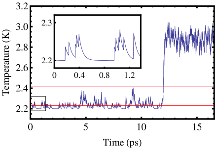
Figure 4: Trace of a typical central segment temperature trajectory $T(t)$, with a switching event at $t\sim 20\,\text{ps}$ FN:parameters . Overlaid on the trace are red lines showing the temperatures $T_{\text{sc}}$ (lowest), $T_{\text{sp}}$ (middle), and $T_{\text{rs}}$ (highest) corresponding to the superconducting minimum, the saddle-point, and the resistive minimum of the effective potential. The inset shows a blow-up of the boxed region of the main figure.

A picture of a switching event can be constructed by analyzing the real-time dynamics of the Langevin equation. A typical trace of the temperature of the central segment as a function of time $T(t)$, evolving according to Eq. (14), is depicted in Fig. 4. To obtain this trace we integrate Eq. (14) forward in time, numerically, starting with the initial condition $T(t=0)=T_{\text{b}}$. Phase slips correspond to sharp rises of $T(t)$, and cooling to gradual declines of $T(t)$. The two minima, $T_{\text{sc}}$ and $T_{\text{rs}}$, as well as the local maximum $T_{\text{sp}}$ of the fictitious potential $U(T)$, are indicated by the red lines. From the trace, it can be seen that the temperature of the system starts by spending a long time in the vicinity of $T_{\text{sc}}$, until a burst of phase slips pushes it “over” $T_{\text{sp}}$ and the temperature quickly progresses towards the vicinity of $T_{\text{rs}}$.

The fundamental quantity of interest is the mean switching time, i.e., the average time required for the wire to switch from being superconductive to resistive. Assuming that the entire wire has temperature $T=T_{\text{b}}$ when the current $I$ is turned on at time $t=0$, we define a switching event as the first time at which $T$, the temperature of the central segment of the wire, exceeds the temperature $T^{\ast}$, where $T_{\text{sp}}\ <T^{\ast}\leq T_{\text{rs}}$. With this definition, the mean switching time corresponds to the Mean First Passage Time $\tau(T_{\text{b}}\ \rightarrow T^{\ast})$ to go from the bath temperature $T_{\text{b}}$ to the temperature $T^{\ast}$. In the case of weak fluctuations, the problem is indeed a barrier crossing problem, i.e., the system spends a long time in the vicinity of the starting temperature $T_{\text{b}}\sim T_{\text{sc}}$, until a burst of phase slips propels it over the barrier at $T_{\text{sc}}$. After $T_{\text{sc}}$ is exceeded, the system moves quickly (compared to the barrier-crossing time) towards $T_{\text{rs}}$. Therefore, the mean switching time will only have a weak dependence on $T^{\ast}$, provided $T^{\ast}$ is significantly higher than $T_{\text{sp}}$, as this is the temperature range in which the system is moving relatively quickly towards the high-temperature steady state.

V Formalism for addressing switching dynamics: Mean first passage time

In the previous section, we have shown that the Mean First Passage Time (MFPT) for the temperature $T$ in the central segment to exceed a critical value $T^{\ast}$ can be used to characterize the switching from the superconducting to the resistive state. In this section, we develop the tools for computing the MFPT in two steps. In the first step, we derive the Master Equation associated with the Langevin equation 14. In the second step, we use the Master Equation to obtain a delay-differential equation directly for the MFPT $\tau(T)\left[\equiv\tau(T\rightarrow T^{\ast})\right]$ as a function of the initial temperature $T$.

V.1 Master Equation

We now derive the Master Equation associated with the Langevin equation (14). The Master Equation is a delay-differential equation that describes the evolution of the probability density $P(T,t)$ for the central segment of the nanowire to have temperature $T$ at time $t$. Note that by the term “delay” we actually mean a delay in temperature. That is, the evolution of $P(T,t)$ is non-local in temperature but local in time. Before delving into the derivation, we quote the result:

$$\partial_{t}P(T,t)= \partial_{T}\,[(T-T_{\text{b}})\,\alpha(T)\,P(T,t)]-\Gamma(T)\,P(T,t)$$

$$+\Gamma\big{(}T-\widetilde{\eta}(T)\big{)}\,P\big{(}T-\widetilde{\eta}(T),t\big{)}\times$$

$$\quad\quad\quad\quad\quad\quad\quad\quad\quad\times\big{(}1-\partial_{T}\,\widetilde{\eta}(T)\big{)},$$ (19)

where the first (i.e., the transport) term corresponds to the effect of cooling, and the last two terms correspond to the effects of heating. We remind the reader that, $\widetilde{\eta}(T)$ is defined as the temperature change due to a phase slip, such that after the phase slip the central segment temperature becomes $T$.

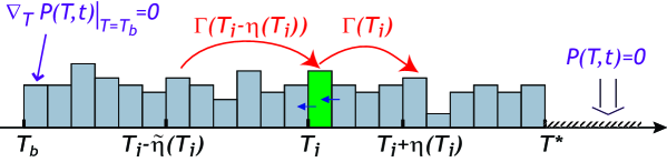
Figure 5: Schematic diagram showing the probability $P(T_{j},t)$ to find the system in the temperature interval $(T_{j},\,T_{j}+\Delta T)$ indicated by gray blocks. Processes involved in the rate of change of the probability in the $i-\text{th}$ interval (green block) are represented by blue arrows (cooling) and red arrows (heating by phase-slips). The boundary conditions at the ends of the temperature interval $(T_{\text{b}},\,T^{\ast})$ for computing the Mean First Passage Time are indicated in purple.

The probability distribution $P(T,t+dt)$ at temperature $T$ and time $t+dt$ is related to $P(T,t)$ at an earlier time $t$ by the two effects: (a) cooling, and (b) heating, as summarized in Fig. 5. To understand these effects, we begin by discretizing the temperature interval into equally wide slices $T_{i}$ of width $dT$, indexed by $i$.

To understand the effect of cooling, we consider the change in the probability of finding the system in the $i$-th temperature slice, $P(T_{i},t+dt)-P(T_{i},t)$. Due to cooling, some of the probability in slice $i+1$ will move into the $i$-th slice at a rate $(T_{i+1}-T_{b})\,\alpha(T_{i+1})/dT$. Concurrently, some of the probability slice $i$ will move into slice $i-1$ at a rate $(T_{i}-T_{b})\,\alpha(T_{i})/dT$. These two processes are indicated by the blue arrows in Fig. 5. By adding these two rates, we find

$$\partial_{t}P(T_{i},t)=\frac{1}{dT} [(T_{i+1}-T_{b})\,\alpha(T_{i+1})\,P(T_{i+1},t)$$

$$-(T_{i}-T_{b})\,\alpha(T_{i})\,P(T_{i},t)].$$ (20)

To find the continuum version of this equation we take the limit $dT\rightarrow 0$, thus arriving at

$$\partial_{t}P(T,t)=\partial_{T}[(T-T_{b})\alpha(T)P(T,t)],$$

where we have identified the definition of the $T$ derivative when taking this limit on the right hand side of Eq. (20).

On the other hand, heating is caused by discrete phase-slips, which occur at a temperature- and current-dependent rate $\Gamma(T,I)$. Heating decreases the probability in the $i$-th slice, $P(T_{i},t)$, at the rate $\Gamma(T_{i},I)\,P(T_{i},t)$, as the probability is boosted to higher temperatures by phase-slips. On the other hand, $P(T_{i},t)$ increases, as probability from lower temperatures, $\widetilde{T}\approx T_{i}-\widetilde{\eta}(T_{i})$, gets boosted to $T_{i}$ due to heating. These two heating processes are indicated by the red arrows in Fig. 5. To compare these two rates, we must take care of the fact that the boost is temperature dependent, and thus there may be some ‘stretching’ of the corresponding temperature intervals before and after the boost. Consider the temperature interval $(T_{i},\,T_{i}+dT)$ after the boost. What is the corresponding temperature interval before the boost? Using the ‘un-boost function’ $\widetilde{\eta}$, we find the interval to be

$$\big{(}T_{i}-\widetilde{\eta}(T_{i}),\,T_{i}+dT-\widetilde{\eta}(T_{i}+dT)\big{)}.$$ (21)

Therefore, the width of the interval before the boost is approximately $(1-\partial_{T_{i}}\,\widetilde{\eta}(T_{i}))dT$ and not $dT$. Thus, after taking the continuum limit we find that the probability density $P(T)$ increases at the rate

$$(1-\partial_{T}\,\widetilde{\eta}(T))\,f(T-\widetilde{\eta}(T))\,P(T-\widetilde{\eta}(T),t).$$

Combining the rates of in- and out-flux of the probability-density due to cooling and heating effects, we obtain the master equation given as Eq. (19).

V.2 Mean First Passage Time

The fundamental quantity that we want to compute is the Mean First Passage Time (MFPT) $\tau(T_{\text{b}}\ \rightarrow T^{\text{*}})$. In this subsection, we use the master equation (19), as a starting point for obtaining a delay-differential equation directly for $\tau(T)\equiv\tau(T\rightarrow T^{\text{*}})$. We proceed using a straightforward generalization of the standard procedure to systems with jump processes (i.e., those that have master equations with delay terms) Gardiner ; Kampen .

We begin by supplementing the Master Equation with the boundary conditions appropriate for computing the MFPT. When computing the MFPT, we want to remove any element from the ensemble once its temperature reaches one of the boundaries of the interval. Thus, we would typically impose absorbing wall boundary conditions on both sides of the interval at $T_{\text{b}}$ and $T^{\ast}$, i.e., $P(T_{\text{b}},t)=P(T^{\ast},t=0)$. However, because we have a jump process, which transfers probability-density from lower temperatures to higher temperatures, we must instead impose the absorbing segment boundary condition

$$P(T,t) =0, \text{for }T>T^{*},$$ (22)

beyond the upper end of the interval, so as to capture systems in which the temperature gets boosted beyond the upper end of the interval by the jump process. The dynamics described by Eq. (19) is also peculiar in another way. If we choose $T_{\text{b}}$ as the temperature at the lower end of the interval then there are no processes that can cause a passage through the lower end of the interval, as can be seen from the Langevin equation (14). Thus, at the lower end of the interval, instead of the absorbing wall boundary condition, we must impose the no flux boundary condition

$$\partial_{T_{\text{b}}}P(T_{\text{b}},t) =0.$$ (23)

These boundary conditions, (22) and (23), are indicated (in purple) in Fig. 5. We note that the probability density may be discontinuous at the upper boundary, due to the jump process.

With the boundary conditions in hand, we consider the integrated probability density function

$$G(T^{\prime},t)=\int_{T_{\text{b}}}^{T^{*}}dT\,P(T,t|T^{\prime},0).$$ (24)

Here, we have generalized from the probability $P(T,t)$ to the conditional probability $P(T,t|T^{\prime},0)$ of finding the system to be at temperature $T$ at time $t$, subject to the boundary conditions, if it started out at temperature $T^{\prime}$ at time $0$. Then the function $G(T^{\prime},t)$ measures the probability that a system that started out at temperature $T^{\prime}$ has never left the temperature interval $(T_{\text{b}},\,T^{\ast})$ while the time $t$ has passed. In particular, the rate of first passages out of the interval $(T_{\text{b}},\,T^{\ast})$ at time $t$ is given by $-\partial_{t}G(T^{\prime},t)$. Therefore, the MFPT $\tau(T^{\prime})$ for a system that starts at temperature $T^{\prime}$ is given by

$$\tau(T^{\prime}) =\int_{0}^{\infty}dt\,t\left(-\partial_{t}G(T^{\prime},t)\right)$$ (25)

$$=\int_{0}^{\infty}dt\,G(T^{\prime},t),$$ (26)

where the surface term resulting from an integration by parts is assumed to be zero, as all the “particles” are assumed to be able to leave the interval in the long-time limit.

Next, we obtain a differential equation for $\tau(x)$ by appropriately integrating the backwards-in-time master equation, i.e., the equation

$$\partial_{t^{\prime}}P(T,t|T^{\prime},t^{\prime})=(T^{\prime}-T_{\text{b}})\,\alpha(T^{\prime})\,\partial_{T^{\prime}}P(T,t|T^{\prime},t^{\prime})+\Gamma(T^{\prime})\left[P(T,t|T^{\prime},t^{\prime})-P(T,t|T^{\prime}+\eta(T^{\prime}),t^{\prime})\right].$$ (27)

Taking advantage of the fact that the present stochastic process is homogeneous in time, we transfer the time-derivative on the left hand side of Eq. (27) to the $t$ variable from the $t^{\prime}$ variable:

$$\partial_{t^{\prime}}P(T,t|T^{\prime},t^{\prime}) =+\partial_{t^{\prime}}P(T,t-t^{\prime}|T^{\prime},0)$$ (28)

$$=-\partial_{t}P(T,t-t^{\prime}|T^{\prime},0).$$ (29)

By substituting Eq. (29) into Eq. (27) and integrating both sides with respect to $T^{\prime}$ over the interval $(T_{\text{b}},\,T^{\ast})$, we arrive at an equation for $G(T^{\prime},t)$:

$$\partial_{t}G(T^{\prime},t) =(T_{\text{b}}-T^{\prime})\,\alpha(T^{\prime})\,\partial_{T^{\prime}}G(T^{\prime},t)$$ (30)

$$-\Gamma(T^{\prime})\left[G(T^{\prime},t)-G(T^{\prime}+\eta(T^{\prime}),t)\right].$$ (31)

Finally, we integrate over all times to obtain an explicit delay-differential equation for the MFPT:

$$(T_{\text{b}}-T^{\prime})\,\alpha(T^{\prime})\,\partial_{T^{\prime}}\tau(T^{\prime})$$ (32)

$$-\Gamma(T^{\prime}) \left[\tau(T^{\prime})-\tau(T^{\prime}+\eta(T^{\prime}))\right]=-1,$$

where we have used Eq. (26) to identify $\tau(T^{\prime})$ on the left hand side, and the assumption that $P(T,t|T^{\prime},0)$ tends to zero in the long-time limit on the right hand side.

The delay differential equation (32), together with the boundary conditions (22) and (23), may be conveniently solved numerically by using the shooting method. The key to this method lies in taking advantage of the fact that in the nonlocal term $\Gamma(T^{\prime})\,\tau(T^{\prime}+\eta(T^{\prime}))$, the factor $\eta(T^{\prime})$ is always positive. Therefore, by integrating from high temperatures to low temperatures, we can always look up the value of the non local term from the region where integration has already been carried out. We implement the shooting procedure as follows: (1) pick a value for $\tau(T^{\ast})$; (2) shoot towards lower temperatures to obtain $\partial_{T_{\text{b}}}\tau(T_{\text{b}})$; and (3) adjust $\tau(T^{\ast})$ until the boundary condition $\partial_{T_{\text{b}}}\,\tau(T_{\text{b}})=0$ is satisfied.

VI Switching behavior of superconducting nanowires: results and interpretations

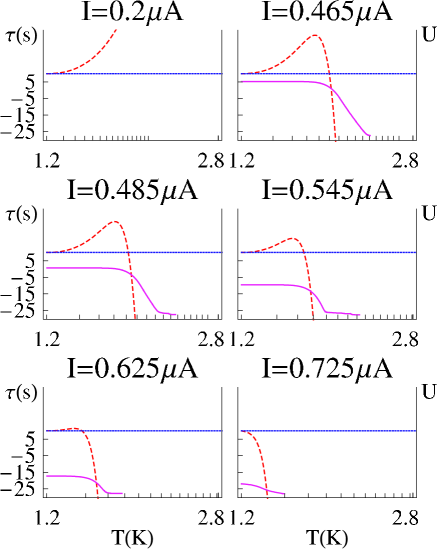
Figure 6: Numerical solutions of the Mean First Passage Time Eq. (32), as functions of the central segment temperature $T$, for bath temperature $T_{\text{b}}=1.2\,\text{K}$ and several values of the bias current between $0.2$ and $0.725\,\mu\text{A}$ (solid pink) FN:parameters . For comparison, superposed on the MFPT plots are the effective potential that appears in Eq. (18) (dashed red lines). The solid blue lines correspond to the zero of the effective potential. The hash marks on the temperature axes correspond to the sequence of temperatures given by Eq. (33).

VI.1 Properties of solutions of the Mean First Passage Time equation

The Mean First Passage Time $\tau(T^{\prime}\rightarrow T^{\ast})$ for a system that starts out at temperature $T^{\prime}$ to exceed the temperature $T^{\ast}$ is described by the delay-differential equation (32), together with the boundary conditions (22, 23). The mean switching time corresponds to the MFPT $\tau(T_{\text{b}}\ \rightarrow T^{\ast})$. To understand the solutions of the MFPT equations, we remind the reader that $T^{\ast}$ must be chosen to be a temperature sufficiently far above the saddle-point temperature $T_{\text{sp}}$ of the effective potential (cf. Fig. 3) that the MFPT has only a weak dependence on $T^{\ast}$. Solutions of the MFPT equations for several values of the bias current are plotted in Fig. 6, along with the corresponding effective potentials. The solutions have the following structure:

• In the temperature interval $T_{\text{b}}<T<T_{\text{sp}}$ the MFPT is largely independent of the temperature $T$.

• For $T$ in the vicinity of $T_{\text{sp}}$ the MFPT drops sharply.

• In the temperature interval $T_{\text{sp}}<T<(T^{\ast},T_{\text{rs}})$ the MFPT is again largely independent of $T$.

The origin of this structure can be seen in the real-time dynamics depicted in Fig. 4. Systems that start at temperatures below the barrier temperature $T_{\text{sp}}$ in the effective potential must diffuse over it, which is a very slow process. The MFPT in the interval $T_{\text{b}}<T<T_{\text{sp}}$ is correspondingly large. Furthermore, the MFPT is largely independent of the initial temperature, as this interval is essentially ergodic, i.e., a system that starts in this interval typically spends a lot of time exploring the entire interval before leaving it. On the other hand, a system that start at some temperature above the barrier in the effective potential rolls down the potential gradient relatively quickly before reaching $T^{\ast}$. Therefore, in terms of temperatures increasing from $T_{\text{b}}$, the MFPT starts out essentially constant over the ergodic interval, and then drops sharply as $T$ crosses the barrier in the effective potential, before finally flattening out at temperatures higher than $T_{\text{sp}}$.

We note that it is numerically advantageous to set $T^{\ast}$ to be as low as possible in the high-temperature (i.e., flat MFPT) regime, so as to avoid instabilities in the numerical integration of Eq. (32).

VI.2 Number of phase slips in a thermal runaway train

In this subsection, we consider the question of exactly how many phase-slips it takes to form a runaway train. Let us start our discussion by first turning off the (deterministic) cooling term in the stochastic equation (14). If we now start with an initial temperature $T_{0}$, then the sequence

$$T_{0},\,T_{0}+\eta(T_{0}),\,T_{0}+\eta(T_{0})+\eta(T_{0}+\eta(T_{0})),\,...$$ (33)

defines the discrete sequence of values that phase-slips would cause $T$ to jump to, as marked on the horizontal axes in Fig. 6 for $T_{0}=T_{\text{b}}$. The probability per unit time $\Gamma(T)$ to make a jump changes at each step, and so does the size $\eta(T)$ of the jump, owing to their explicit dependence on temperature. On the other hand, if we turn off the heating term then we would have a deterministic problem in which $T$ would decay at a rate $\alpha(T)$, from its initial value $T_{0}>T_{\text{b}}$ to the bath temperature $T_{\text{b}}$. It is the competition between the discrete heating and continuous cooling that makes for a rather rich stochastic problem.

The number of tick marks [see sequence (33)] between $T_{\text{b}}$ and $T^{\text{*}}$ (see Fig. 6) is nothing but the of number $N(T_{\text{b}},I)$ of phase-slip events required to raise the temperature of the central segment from $T_{\text{b}}$ to $T^{\text{*}}$ in the absence of cooling. Accordingly, $N(T_{\text{b}},I)$ also provides an estimate of the number of phase-slip events needed to overcome the potential barrier, if the time-span of these events were insufficient to allow significant cooling to occur. “Thermal runaway”—heating by rare sequences of closely-spaced phase slips that overcome the potential barrier—constitutes the mechanism of the superconductive-to-resistive switching within our model. As the number $N(T_{\text{b}},I)$ of phase-slips needed increases, the total number of phase-slip events taking place before a switching event occurs, and correspondingly the value of the mean switching time $\tau_{\text{s}}\ (T_{\text{b}},I)$, may indeed become quite large.

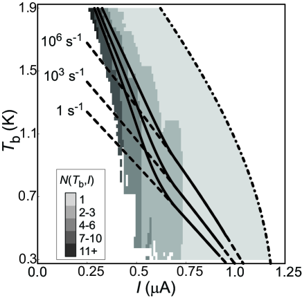
Figure 7: Map of $N(T_{b},I)$, i.e., the number of consecutive phase slips required to overcome the barrier and induce the wire to switch, as a function of bias current $I$ and bath temperature $T_{b}$. The three solid lines are contours along which $\Gamma_{\text{sw}}^{-1}$ (the mean switching rate) is $1$, $10^{3}$, and $10^{6}$ $\text{s}^{-1}$. Similarly, the three dashed lines are contours along which the phase slip-rate is $1$, $10^{3}$, and $10^{6}$ $\text{s}^{-1}$. For comparison, the de-pairing critical current is indicated by the dashed-dotted line.

The map of the number $N(T_{\text{b}},I)$ of phase slips needed over the $I$-$T_{\text{b}}$ plane is presented in Fig. 7. The progression from smaller to larger $N(T_{\text{b}},I)$ corresponds to the progression from lighter to darker shading. For clarity of presentation we have grouped together a few values of $N(T_{\text{b}},I)$. We see from the figure that, as the bias current is increased, one traverses through regions of decreasing $N(T_{\text{b}},I)$. It is important to observe that the typical value of $N(T_{\text{b}},I)$ is only ten or fewer. The smallness of this number highlights why going beyond continuous Joule heating to the discrete phase-slip model is crucial for our analysis.

Remarkably, there is a region in the $I$-$T_{\text{b}}$ plane within which the occurrence of just one phase-slip is sufficient to cause the nanowire to switch from the superconductive to the resistive state. We denote this this region as the “single phase-slip switching regime”. A switching measurement in this range can in fact provide a way of detecting and probing an individual phase-slip fluctuation.

VI.3 Mean switching time

Let us begin by considering the single phase-slip switching regime identified in the previous subsection. In this regime, the value of the mean switching time is dictated purely by the probability for a phase-slip event to occur at a given bath temperature $T_{\text{b}}$ and by the bias current $I$. The mean switching rate is thus identical to the phase-slip rate (which is an input quantity in our theory):

$$\tau_{\text{s}}^{-1} =\Gamma,$$ “single phase-slip switching regime.” (34)

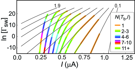
Figure 8: Logarithm of the mean switching rate, $\ln\Gamma_{\text{sw}}$, as a function of current for bath temperatures $T_{b}=0.1,\,0.3,\,0.5\,...,1.9\,\text{K}$.

As we move beyond the “single phase-slip switching regime,” several phase-slip events become necessary for switching. The mean switching rate $\tau_{\text{s}}^{-1}$ thus begins to deviate from $\Gamma$ to a value below $\Gamma$, as can be seen from Fig. 8. For concreteness, we have assumed that the phase-slip fluctuations are thermally activated, and have used the form of $\Gamma$ as given by the LAMH theory for the current-biased case. (The precise expression is provided in Appendix A.)  The deviation of $\tau_{\text{s}}^{-1}$ from $\Gamma$ can be interpreted in terms of the evolution in the number of phase slips $N(T_{\text{b}},I)$, which was discussed in the previous subsection. To make the link between the two more evident, we have color-coded the plots according to the value of $N(T_{\text{b}},I)$.

An alternative representation of our results can be obtained by studying the equal-value contours. A graphical representation of the contour lines for a few values of $\tau_{\text{s}}^{-1}$ and $\Gamma$, chosen in an experimentally accessible range, is provided in Fig. 7. Whilst the spacing between the $\Gamma$ contour lines decreases monotonically upon lowering $T_{\text{b}}$, the spacing between the $\tau_{\text{s}}^{-1}$ lines can be seen to behave non-monotonically. In the following subsection we examine a consequence of this non-monotonicity.

VI.4 Switching-current distribution

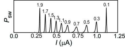
Figure 9: Switching rate $P_{\text{sw}}$ as a function of current for bath temperatures $T_{b}=0.1,\,0.3,\,0.5\,...,1.9\,\text{K}$. The current sweep rate was set to $58\mu\text{A}/\text{s}$.

The mean switching time $\tau_{\text{s}}$ in bistable current-biased systems can be measured directly by performing waiting-time experiments. Alternatively, $\tau_{\text{s}}$ can be extracted from switching-current statistics FultonD1974 . As described in Section II, the switching-current distribution can be generated via the repeated tracing of the $I$-$V$ characteristic, ramping the current up and down at some sweep rate

$$\frac{dI}{dt}=\pm r.$$

The sweep-rate-dependent probability $P(I,T_{\text{b}};r)dI$ for the event of switching (from the superconductive to the resistive branch) to take while the current is in the range $I$ to $I+dI$ is explicitly related to the mean switching time $\tau_{\text{s}}$ via the relation

$$P(T_{\text{b}},I;r)dI =\left(\tau_{\text{s}}^{-1}(T_{\text{b}},I)\frac{dI}{r}\right)\times$$

$$\quad\quad\times\left(1-\int_{0}^{I}P(T_{\text{b}},I^{\prime};r)\text{ }dI^{\prime}\right).$$ (35)

The term in the first pair of parentheses corresponds to the probability for switching to happen within the ramp time, whilst the term in the second pair of parentheses corresponds to the probability that the wire has not already switched before reaching the bias current $I$. By using Eq. (35) we obtain the distribution of switching currents in superconducting nanowires in terms of the theory presented in the present paper. The plots illustrated in Fig. 9 are simply the translation of the mean switching-rate plots shown in Fig. 8, to the switching-current distribution for a chosen value of $r$.

Upon raising $T_{\text{b}}$, one would naïvely expect the distribution of the switching currents to become broader for a model involving thermally activated phase slips. Such broadening of the distribution is indeed obtained up to a crossover temperature scale $T_{\text{b}}^{\text{cr}}(r)$ (i.e., the temperature below which, loosely speaking, switching is induced by single phase slips). However, on continuing to raise $T_{\text{b}}$, but now through temperatures above $T_{\text{b}}^{\text{cr}}(r)$, the distribution-width shows a seemingly anomalous decrease. Based on the discussion of the previous subsection, this can be understood as a manifestation of the now-decreasing spacing between the $\tau_{\text{s}}$ contour lines in the $I$-$T_{\text{b}}$ space.

This striking behavior above $T_{\text{b}}^{\text{cr}}(r)$ may be understood via the following reasoning: the larger the typical number of phase-slips in sequences that induce superconductive-to-resistive thermal runaway, the smaller the stochasticity in the switching process and, hence, the sharper the distribution of switching currents. This non-monotonicity in the temperature dependence of the width of the switching-current distribution, along with the existence of a regime in which a single phase-slip event can be probed, are the two key predictions of our theory. In the following section, we proceed to carry out a detailed comparison of between this theory and the recently performed experiments discussed in Sec. II.

VII Comparison with experiments

In this section, we compare results from the experiments described in Section II with predictions of our theory presented in Sections III-VI. We show that our theory is both qualitatively and quantitatively consistent with experimental observations. The main implications of this comparison are that: (1) the switching-current distribution-width does indeed increase as the temperature is decreased; (2) there is a single phase-slip-to-switch regime at low temperatures; and (3) thermally activated phase-slips, alone, are insufficient to fit the dependence of the mean switching time on the bias current at low temperatures. This suggests that one should include the effects of Quantum Phase-Slips (QPS) Giordano1990 ; BezryadinLT2000 ; upon including quantum phase-slips phenomenologically, we obtain good fits to the experimental data in the low-temperature regime as well. For the purposes of this comparison we use the data from a representative superconducting nanowire; data for more samples may be found in Refs. Sahu2008 ; Sahu2008b . This section is structured as follows. To establish the validity of the thermal hysteresis model, we begin by analyzing the $I$-$V$ hysteresis loops. Next, we qualitatively analyze the experimentally measured switching-current distribution. We continue with a quantitative analysis of the experimental data on the mean switching rate. Finally, we look at the implications of the quantitative analysis, including identifying the single phase-slip-to-switch regime and the scenarios for quantum phase-slips in the low temperature behavior.

VII.1 I-V hysteresis loops

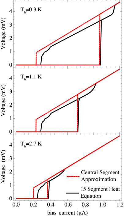
Figure 10: Comparison of $I$-$V$ hysteresis loops computed using central segment approximation and the full heat equations. For the case of the heat equation the wire was split into 15 segments. The steps and upturns in the high voltage branch of the segmented solution correspond to various segments becoming superconducting, and would disappear in the continuum limit. Heat conductivity, phase-slip rate, and geometrical parameters used are listed in Table 1.

We begin our analysis by comparing the qualitative features of the experimentally measured and theoretically computed current-voltage characteristics. Experimentally, it is found that at high temperatures there is no hysteresis. As $T_{\text{b}}$ is lowered, a hysteresis loop gradually opens up. Next, as the temperature is lowered even further, the switching current (i.e., the bias current at the superconducting-resistive transition) grows gradually, whilst the re-trapping current (i.e., the bias current at the resistive-superconducting transition) remains almost unchanged. This behavior is consistent with the experimental observations and theory of Ref. TinkhamFLM2003 , where it is also qualitatively explained as follows. Switching is controlled by the properties of the low-temperature (i.e., superconducting-like) solution of Eq. (2), thus switching depends strongly on the temperature of the bath $T_{\text{b}}$. On the other hand, re-trapping is largely a property of the hotter (i.e., resistive) state, and thus has only a weak dependence on $T_{\text{b}}$.

Typical $I$-$V$ curves obtained from the central segment model [e.g., stationary solutions of Eq. (17)], as well as those obtained from solving the heat equation, are shown in Fig. 10 for several bath temperatures $T_{\text{b}}$. Following Ref. TinkhamFLM2003 , the solutions of the heat equation were obtained from a spatially discretized version of Eq. (2). In both cases, the heat conductivity and the phase-slip rate were obtained from Eqs. (50) and (36), respectively. The theoretical curves both qualitatively and quantitatively reproduce the features seen in experiments TinkhamFLM2003 ; Sahu2008 ; Sahu2008b . We take a moment to point out that in fitting the experimental data it is important to take into account the nonlinear dependence of the phase-slip rate on the bias current. Finally, we point out that making the central segment approximation has little effect on the switching current found in the hysteresis loops (for typical wires used in experiments). This fact supports the validity of the central segment approximation for modeling switching phenomena.

VII.2 Switching current distributions

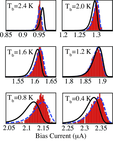
Figure 11: Experimental data (red bar-charts) and theoretical fits (black lines) for the switching-current distributions for various bath temperatures. To make the comparisons between the shapes of distributions easier, we also show theoretical curves shifted so that their means coincide with the experimental curves (blue dashed lines). The fitting parameters used are listed in Table 1.

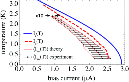
Figure 12: Hierarchy of critical and switching currents. All theoretical curves were produced using the parameters obtained from fitting experimental data. The highest current scale is the de-pairing critical current $I_{\text{c}}(T)$. Next, is $I_{\text{u}}(T)$, the scale for linear instability due to overheating, as described by Eq. (17). Finally, comes the actual switching current $I_{\text{sw}}(T)$. The error bars on the switching current correspond to the $10\times$ the standard deviation of the switching current distribution (the scale of the standard deviation was exaggerated to make it easier to see; the sweep rate was set to $58\,\mu\text{A}/\text{s}$). The fitting parameters used are listed in Table 1.

In the experiments, every time an I-V characteristic is measured by sweeping the bias current up and down, switching occurs at a distinct value of the bias current. By repeatedly measuring the hysteresis loop at a fixed bath temperature $T_{\text{b}}$ and current sweep rate $dI/dt$, one can obtain the distribution of switching currents $P(I_{\text{sw}},T_{\text{b}},dI/dt)$. Typical $P(I_{\text{sw}},T_{\text{b}},dI/dt)$ distributions, obtained experimentally, are shown in Fig. 11. For completeness, we also show the corresponding theoretical fits, which we shall describe in detail in the next subsection. For a given $T_{\text{b}}$, switching events tend, in general, to occur at lower bias currents than the switching current found in the thermodynamic stability analysis of Ref. TinkhamFLM2003 . The reason for this premature switching at bias currents that are lower than the stability analysis indicates is, of course, thermally activated barrier crossing in the form of a phase-slip bursts. In Fig. 12 we plot the mean and the standard deviation of the switching-current distributions measured experimentally, as well as those obtained from theoretical fits of the simplified model. By using the tuning parameters obtained from the fits, we also plot the theoretical de-pairing critical current and the critical current from the stability analysis of the simplified model Eq. (17).

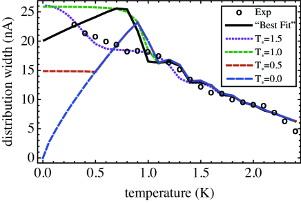
Figure 13: Standard deviation of the switching-current distribution as a function of temperature. Comparison of experimental data for a typical sample (circles) with various QPS scenarios labeled by $T_{\ast}$. The “best fit” curve was obtained by using the parameters given in Table 1, where the fit was optimized to simultaneously capture the temperature-dependence of mean switching current and the standard deviation of the switching current distribution.

As described in the introduction, one would typically expect the standard deviation of the switching-current distribution to decrease with decreasing temperature, as thermal fluctuations become suppressed. Such narrowing of the switching-current distribution is expected to continue with cooling, until the temperature becomes sufficiently low such that quantum phase slips are the main drivers of the switching, at which point the narrowing is expected to come to a halt. Qualitatively, this would indeed be the case if switching was always triggered by a single phase-slip. However, our theory, predicts that the situation is more complicated, because the mean switching time, and hence the width of the switching-current distribution, is controlled by a competition between the phase-slip rate and the number of consecutive phase-slips needed to induce switching, as described in the previous section. Thus, qualitatively, we expect the opposite behavior at higher temperatures. That is, in the regime of thermally activated phase slips and at temperatures above the single phase-slip-to-switch regime, the width of the switching-current distribution should increase with decreasing temperature. This counter-intuitive broadening of the switching current distributions with decreasing temperature is indeed observed experimentally, as shown in Fig. 13.

VII.3 Mean switching rate

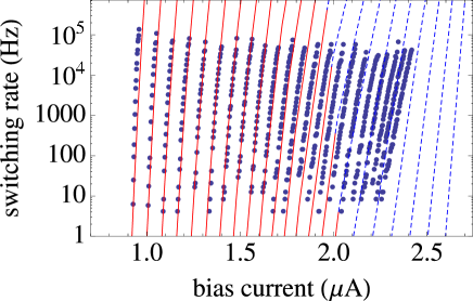
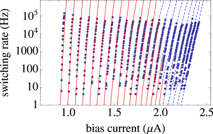
Figure 14: Comparison of theoretical fits (lines) to the experimental (blue dots) Mean Switching Rates. The top panel shows fits with thermally activated phase slips only, whilst the bottom panel includes both thermally activated and quantum phase slips. The solid red lines correspond to multiple-phase-slips-to-switch regime, whilst the dashed blue lines correspond to multiple-phase-slips-to-switch regime. The fitting parameters used are listed in Table 1.

As the switching-current distribution depends on the bias-current sweep-rate, in order to quantitatively compare our theory with experimental data, we focus on the mean switching rate, which is related to the switching current distribution via Eq. (35). The experimentally obtained mean switching rate $\tau^{-1}(I,T_{\text{b}})$ for a typical sample, along with theoretical fits, are plotted as a function of the bias current $I$ for different values of the bath temperature $T_{\text{b}}$ in Fig. 14. To help relate the mean switching rate to the switching current distribution width, we note that for a fixed $T_{\text{b}}$, the shallower the slope of $\tau^{-1}(I,T_{\text{b}})$ the wider the corresponds distribution. The two main features of the experimental data plotted in Fig. 14 are as $T_{\text{b}}$ decreases (1) the mean switching rate decreases ($\langle I_{\text{sw}}\ \rangle$ increases) and (2) the slope of $\tau^{-1}(I)$ decreases ($I_{\text{sw}}$ distribution width becomes wider).

Two different fits to the same set of experimental data are shown in Fig. 14. The fit shown in the top panel includes TAPS only, whilst the one in the bottom panel uses the fitting parameters from the top panel but also includes QPS. The fits were obtained using the fast switching-rate calculation routine described in Appendix C. The tuning parameters that were obtained from the fit are listed in Table 1 and fall into two categories. The first category is composed of the geometric model parameters, such as the wire length, whilst the second category controls the “input functions,” i.e., the heat capacity, the heat conductivity, and the phase-slip rate. The expressions for these input functions are given in Appendix A. We note that in obtaining these fits we verified that the fitting parameters that we used were consistent with the high-temperature $R(T)$ data Sahu2008b .

The TAPS-only fit (top panel of Fig. 14) works well at temperatures above $1\,\text{K}$. In this regime the theory is able to quantitatively explain the observed rise in mean switching current ($\langle I_{\text{sw}}\rangle$) with decreasing temperature, as well as the peculiar increase the $I_{\text{sw}}$ distribution width with decreasing temperatures.

VII.4 Single-slip-to-switch regime

In general, as the temperature is lowered and the bias current increased, the wire tends to enter the single-slip-to-switch regime, as indicated in Fig. 7. This regime roughly corresponds to the region of the $(I,T)$ plane where a single phase slip heats up the wire to $T_{c}(I)$, and thus the boundaries of this regime are primarily determined by the heat capacity of the wire. Within this regime, switching-current statistics correspond directly to the phase-slip statistics.

Theoretical fitting indicates that at temperatures below $\sim 1\,\text{K}$ the wire enters the single-phase-slip-to-switch regime. This regime is indicated by the switch of the theory curves from solid red lines to dashed blue lines in Fig. 14. In the absence of quantum phase slips, in this regime the $I_{\text{sw}}$ distribution width should follow a more conventional behavior, and decreases with temperature. This corresponds to the increase in the slope of the mean switching rate curves with decreasing temperature in the single-slip-to-switch regime (see the top panel of Fig. 14).

However, experimentally the distribution width seems to increase monotonically as the temperature is lowered, even in the single-slip-to-switch regime. This behavior suggests that there is an excess of phase slips at low temperatures.

VII.5 Quantum phase-slip scenarios

We expect that at low temperatures quantum phase-slips will contribute strongly to the switching rate. We model the presence of QPS by adding their rate to the rate of TAPS, so as to obtain the total phase-slip rate which goes into our model:

$$\Gamma_{\text{total}}(I,T)=\Gamma_{\text{TAPS}}(I,T)+\Gamma_{\text{QPS}}(I,T).$$

To model the QPS rate, $\Gamma_{\text{QPS}}(I,T)$, we replace $k_{B}T\rightarrow k_{B}(T_{\ast}+T_{1}T)$ in $\Gamma_{\text{TAPS}}(I,T)$ (see Appendix A.1). Here, $T_{\ast}$ and $T_{1}$ are both treated as fitting parameters. Letting $T_{1}$ be nonzero does somewhat improve the quality of our fits.

We can envision several scenarios for the effect of QPS on the switching current distributions, and these are summarized in Fig. 13. In the absence of QPS, upon lowering the temperatures, once the single-slip-to-switch regime is reached the distribution width will start decreasing with temperature. This type of behavior is demonstrated by the $T_{\ast}=0$ line in Fig. 13. However, in the presence of QPS, the distribution width is expected to saturate at low temperature, with the saturation value controlled by $T_{\ast}$. If, upon cooling, the single-slip-to-switch regime is reached before the temperature reaches $T_{\ast}$, we expect the distribution width to first increase and then decrease before saturating with decreasing temperature (cf. the $T_{\ast}=0.5\,\text{K}$ curve in Fig. 13). On the other hand, if $T_{\ast}$ is reached before the single-slip-to-switch regime is reached, we expect the distribution width to increase monotonically with decreasing temperature (cf. the $T_{\ast}=1.0\,\text{K},\,1.5\,\text{K}$ curves in Fig. 13).

To include QPS in our fitting, we started with parameters obtained by fitting the mean switching rate curves at high temperatures ($T>1\,\text{K}$), as described in the previous subsection (i.e. see top panel of Fig. 14). Next, we optimized $T^{\ast}$ and $T_{1}$ to obtain the best possible fit to the mean switching rate curves at low temperatures as well. The optimal values thus obtained were $T_{\ast}=0.726\,\text{K}$ and $T_{1}=0.4$, which corresponds to the fit shown in the bottom panel of Fig. 14 and the curve labeled “best fit” in Fig. 13.

To fit the experimental data, we must be able to simultaneously match both the mean and the standard deviation of the switching current distribution as a function of temperature. However, we have not been able to get quantitative agreement with both of these quantities, simultaneously, in the low temperature regime. The parameter values of $T_{\ast}=0.726\,\text{K}$ and $T_{1}=0.4$ result in a good fit of the mean but not the standard deviation (see Figs. 13 and 14), whilst the values of $T_{\ast}=1.5\,\text{K}$ and $T_{1}=0$ result in a good fit of the standard deviation (see Fig. 13) but not the mean (not shown).

We conclude this section by noting that, for the nanowire that we fitted, our fitting seems to favor the QPS scenario where $T_{\ast}$ is higher than the temperature corresponding to the onset of the single-slip-to-switch regime.

VIII Concluding Remarks

In conclusion, we have developed a quantitative theory of stochastic switching from the superconducting to the normal state in hysteretic superconducting nanowires. Our theory describes the dynamics of the heating of nanowires by random-in-time phase-slip events, and the cooling of the wire by heat conduction into the leads. In general, a train of phase slips, sufficiently closely spaced in time can cause the nanowire to overheat and switch from the low-temperature (superconducting) branch to the high-temperature (normal) branch.

The main achievement of our theory is that it quantitatively describes the unexpected increase in the switching current distribution with decreasing temperature, as is observed in experiments.

Our theory also predicts that there is a single-slip-to-switch regime at low temperatures. In this regime, a single phase slip always triggers a switching event; thus, by studying the switching statistics one has direct access to the phase slips statistics. Typically, phase-slip properties have been studied by linear-response measurements, which are only feasible when the nanowires have a measurable resistance, i.e., at high temperatures. The single-slip-to-switch regime is interesting because it occurs at low temperatures, and thus it is a complementary tool with which to study the properties of phase slips.

Finally, the monotonic increase of the switching current distribution width with decreasing temperature, even in the single-slip-to-switch regime, seems to indicate a severe excess of phase slips over the predictions of the Langer-Ambegaokar McCumber-Halperin model of thermally activated phase slips. It seems at the very least plausible that the quantum tunneling of the superconducting order parameter (i.e., QPS) is the mechanism that serves to meet this excess Sahu2008 .

Appendix A Input functions and parameters

In this appendix we catalog the models for the phase-slip rate, heat capacity, and thermal conductivity that go into the stochastic heat equation (5).

A.1 Phase-slip rate

We begin by considering the phase-slip rate. For the TAPS rate, $\Gamma_{\text{TAPS}}$, we have used the LAMH model, including the nonlinear current response:

$$\Gamma_{\text{TAPS}}(I,T) =\Gamma_{-,\text{TAPS}}(I,T)-\Gamma_{+,\text{TAPS}}(I,T),$$ (36)

$$\Gamma_{\pm,\text{TAPS}}(I,T) =\Omega_{\pm}(I,T)\exp\left(-\frac{\Delta F_{\pm}(I,T)}{k_{B}T}\right),$$ (37)

where $+$ or $-$ indicate whether the phase slip results in current rise or drop, respectively. The phase-slip barriers $\Delta F_{\pm}$ at bias current $I$ and temperature $T$ are given by

$$\Delta F_{-}(T) =C_{1}(T)\left(\frac{8}{3}\sqrt{2}\sqrt{1-3k^{2}}-8k(1-k^{2})\arctan\frac{\sqrt{1-3k^{2}}}{\sqrt{2}k}\right),$$ (38)

$$\Delta F_{+}(T) =C_{1}(T)\left(\frac{8}{3}\sqrt{2}\sqrt{1-3k^{2}}+8k(1-k^{2})\left[\pi-\arctan\frac{\sqrt{1-3k^{2}}}{\sqrt{2}k}\right]\right),$$ (39)

$$C_{1}(T) =\frac{3\sqrt{3}}{8}\frac{\hbar}{2e}I_{c}(T),$$ (40)

where the phase gradient $k$ at current $I$ is the real solution of the equation

$$\frac{I}{I_{c}(T)}=k(1-k^{2}),$$ (41)

and the temperature-dependent critical current $I_{c}(T)$ Bardeen1962 is expressed in terms of the wire length $L$, the critical temperature $T_{c}$, the zero-temperature coherence length $\xi_{0}$, and the normal-state resistance of the wire $R_{n}$ TinkhamL2002 , via

$$I_{C}(T)=(92\,\mu\text{A})\frac{LT_{c}}{R_{n}\xi_{0}}\left(1-\left(\frac{T}{T_{c}}\right)^{2}\right)^{3/2}.$$ (42)

We approximate the prefactor $\Omega_{\pm}(I,T)$ in Eq. (37) via

$$\Omega(T) =\frac{\sqrt{3}}{2\pi^{3/2}}\frac{L}{\xi(T)\,\tau(T)}\left(\frac{\Delta F(I=0,T)}{k_{B}T}\right)^{1/2},$$ (43)

$$\Omega_{-}(I,T) =(1-\sqrt{3}k)^{15/4}\,(1+k^{2}/4)\,\Omega(T),$$ (44)

$$\Omega_{+}(I,T) =\Omega(T).$$ (45)

In the presence of a bias current $I$, the “+” phase slips are exponentially more rare than the “-” phase slips. Therefore, we keep the current-dependent corrections to the prefactor for the “-” phase slips, but not for the “+” phase slips. Thus, we obtain an approximation that works in both the linear-response regime, where the current correction is irrelevant, and in the high-bias regime, where “+” phase slips are rare. We estimate the temperature-dependent coherence length and the Ginzburg-Landau relaxation time via

$$\xi(T) =\xi_{0}\frac{\sqrt{1-(T/T_{c})^{4}}}{1-(T/T_{c})^{2}},$$ (46)

$$\tau(T) =\frac{\pi\hbar}{8k_{B}(T_{c}-T)}.$$ (47)

Thus, we can express the phase-slip rate via the physical parameters $L$, $R_{n}$, $\xi_{0}$, $T_{c}$. To obtain the quantum phase-slip rate, we replace $\Delta F/k_{B}T$ in in Eqs. (37) and Eq. (43) by $\Delta F/k_{B}T_{\text{eff}}$ where $T_{\text{eff}}\equiv(T_{*}+T_{1}T)$ is the effective temperature. $T_{*}$ and $T_{1}$ are treated as fitting parameters, $T^{*}$ being the low-temperature limiting value of $T_{\text{eff}}$.

A.2 Heat capacity and thermal conductivity

Unfortunately, we know of no direct experimental data on the heat capacity and thermal conductivity of current-carrying superconducting nanowires. The diameter of the wires used in experiments is comparable to $\xi_{0}$. Thus, the thermodynamic properties of these wires should lie somewhere between those of a bulk superconductor and a normal metal. Therefore, for the purposes of computing the thermodynamic functions, we model the wire as being composed of a BCS superconducting wire of cross-sectional area $A_{1}$ in parallel to a normal-metal wire of cross-sectional area $A_{2}$. The BCS and Fermi liquid expressions for heat capacity Tinkham are

$$C_{v,\text{BCS}}(\Theta) =-\frac{2N_{0}}{\Theta}\int E_{k}\frac{df_{k}}{d(\beta E_{k})}\left(E_{k}+\beta\frac{dE_{k}}{d\beta}\right)d\xi_{k},$$ (48)

$$C_{v,\text{FL}}(\Theta) =\frac{2}{3}\pi^{2}N_{0}k_{B}^{2}\Theta,$$ (49)

where $\beta=1/k_{B}\Theta$, $E_{k}=\sqrt{\xi_{k}^{2}+\Delta^{2}(\Theta)}$, $f_{k}$ is the Fermi function, and $\Delta(\Theta)$ is obtained from the BCS gap equation. Thus, the total heat capacity of the wire $C_{v}$ is given by

$$C_{v}=\frac{A_{1}C_{v,\text{BCS}}+A_{2}C_{v,\text{FL}}}{A_{1}+A_{2}}.$$ (50)

Similarly, the dirty-limit BCS BardeenRT1959 ; Kopnin2001 and Fermi-liquid expressions for thermal conductivity are

$$K_{s,\text{BCS}}(\Theta) =2N_{0}D\int_{\Delta}^{\infty}\frac{\text{sech}^{2}\left[\epsilon/2k_{B}\Theta\right]}{2k_{B}\Theta}\frac{\epsilon^{2}}{k_{B}\Theta}d\epsilon,$$ (51)

$$K_{s,\text{FL}}(\Theta) =\frac{L_{0}\Theta L}{AR_{n}},$$ (52)

where $D$ is the diffusion constant (for MoGe $D\sim 1\,\text{cm}^{2}/\text{s}$ Graybeal1985 ), and $L_{0}=\pi^{2}k_{B}^{2}/3e^{2}$. The total thermal conductivity $K_{s}$ is, correspondingly, given by

$$K_{s}=\frac{A_{1}K_{s,\text{BCS}}+A_{2}K_{s,\text{FL}}}{A_{1}+A_{2}}.$$ (53)

The fitting parameters describing the heat capacity and thermal conductivity are the cross-sectional areas $A_{1}$ and $A_{2}$, and $T_{c}$ of the nanowire.

Appendix B Fitting procedure

type	parameter name	symbol	value
geometric	wire length	$L$	$110\,\text{nm}$
geometric	central segment length	$L_{1}$	$110\,\text{nm}$
geometric	end segment length	$L_{2}$	$27.5\,\text{nm}$
input function	transition temperature	$T_{c}$	$3.872\,\text{K}$
input function	zero temperature transition length	$\xi_{0}$	$5\,\text{nm}$
input function	QPS effective temperature	$T_{\text{eff}}=T^{*}+T_{1}T$	$0.726\,\text{K}+0.4\,T$
input function	effective superconducting cross-sectional area	$A_{1}$	$320.4\,\text{nm}^{2}$
input function	effective normal cross-sectional area	$A_{2}$	$19.0\,\text{nm}^{2}$
input function	normal state resistance	$R_{n}$	$2666\,\Omega$

Table 1: Parameters used in the switching rate model. Parameters fall into two categories: geometric parameters and input function parameters. The former define the simplified model of the wire, while the latter define the phase slip rate, heat capacity and heat conductivity. Not all of these are used as tuning parameters, as $R_{n}$ and $L$ can be measured directly, and the fitting is only weakly effected by $L_{1}$ and $L_{2}$. Fitting parameters for a representative experimental sample (corresponding to Figs. 11, 12, 13, 14) are displayed in the right hand column.

The main goal of the fitting procedure is to fit the switching-rate data. However, in addition to the mean switching rates at high bias currents and low temperatures, we also have data on the linear-response resistivity in the high-temperature regime. (The linear response resistivity becomes too small to measure below $T\sim 1.9\,\text{K}$ for our wires.) The fitting is performed in two steps. In the first step, we fit the high-temperature linear-response data. In the second step, we use the parameter values from the first step as a starting point in fitting the switching-rate data. Table 1 lists the parameters that go into our model; the procedure for determining them is explained below.

We fit the high-temperature linear-response by conductivity following the usual procedure TinkhamL2002 . In this procedure, $L$ and $R_{n}$ are obtained from microscopy and electrical measurements of the wire resistance above $T_{c}$. We fit the $R(T)$ data using

$$R=\lim_{I\rightarrow 0}\frac{V}{I}=\lim_{I\rightarrow 0}\frac{1}{I}\,\Phi_{0}\,\Gamma_{\text{TAPS}}(I,T)$$

to obtain $T_{c}$ and $\xi_{0}$.

Next, we use the values of $L$, $R_{n}$, $\xi_{0}$, and $T_{c}$, obtained in the first step, as a starting point in fitting of the mean switching-rate data. In this step, we tune $A_{1}$, $A_{2}$, $T_{c}$, $\xi_{0}$, $T^{*}$, and $T_{1}$ simultaneously to obtain the best possible fit over the entire current and temperature range. During this procedure, we set $L_{1}=L$ and $L_{2}=L/4$. We find that variation of $L_{1}$ and $L_{2}$ does not significantly effect the fit, and thus we exclude them from the already-extensive list of fitting parameters.

Finally, we verify that the fitting parameters obtained from fitting the mean switching-time data are consistent with the high-temperature linear-response data.

Appendix C Fast mean first passage time calculation

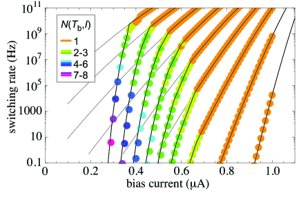
Figure 15: To compare approximate (thick solid lines) and exact (colored dots) methods for solving for the mean switching time delay-differential equation, we plot the mean switching rate $\tau^{-1}(T_{\text{b}},I)$ as a function of bias current $I$ for various bath temperatures $T_{\text{b}}=\{1.9,\,1.7,\,1.5,\,1.3,\,1.1,\,0.9,\,0.7,\,0.5,\,0.3\}$ (from left to right) FN:parameters . The thin lines correspond to the phase-slip rate, and are shown for comparison. The parameter $k$ in Eq. [57] was set to $0.5$.

In this subsection, we develop an approximation for computing the mean switching time very quickly. This approximation models the formation of a phase-slip train, and is useful for fitting experimental data, where it is important to compute the mean switching time for a lot of points $(T_{\text{b}},\,I)$quickly.

In constructing this approximation we make several assumptions. First, we assume that the phase-slip trains are dilute in time, i.e., the wire spends most of its time at the temperature $T_{\text{b}}$, but very rarely there are trains of phase slips that heat up the wire. These trains are not overlapping, i.e., each train either leads to thermal run-away (a successful train) or the wire cools back down to $T_{\text{b}}$ (an unsuccessful train). The train is considered successful if the wire temperature exceeds $T^{\ast}$, as defined in Section IV.

In order to compute the switching rate, we must compute the probability for the formation of a successful phase-slip train $S(T_{\text{b}},I)$ and multiply it by the phase-slip rate $\Gamma(T_{\text{b}},I)$, which corresponds to the rate of formation of the first phase slip in a train. Thus the switching rate is given by

$$\tau^{-1}(T_{\text{b}},I)=S(T_{\text{b}},I)\Gamma(T_{\text{b}},I).$$ (54)

At this point, we make the additional assumption that the probability to form a successful train can be computed phenomenologically, as follows. Consider a phase slip in a wire that is at temperature $T$. Immediately after a phase slip, the wire has temperature $T+\eta(T,I)$, but it is also cooling at the rate $r_{c}=(T-T_{\text{b}})\,\alpha(T,T_{\text{b}})$. If the phase slip-train is to continue, there must be another phase slip within a time $\sim r_{c}^{-1}$; otherwise the wire would cool to the bath temperature $T_{\text{b}}$ and the phase-slip train would be unsuccessful. Applying this procedure to a chain of phase slips, we find that $S(T_{\text{b}},I)$, the probability to construct a successful phase-slip train, is given by

$$S(T_{\text{b}},I)\sim\prod_{i=1}^{N}\frac{\Gamma(T_{i},I)}{(T_{i}-T_{\text{b}})\alpha(T_{i},T_{\text{b}})}.$$ (55)

The mean switching rate, computed using the phenomenological model for the probability to form a successful phase slip train given by Eq. (55), turns out to be too crude to give results that are quantitatively accurate, although, qualitatively, the exact results obtained by solving Eq. (32) are well reproduced. In order to improve accuracy, we take into account the fact that the phase-slip rate drops as the wire cools, and also introduce the tunable parameter $k$, which characterizes how much the wire is allowed to cool before a phase-slip train is considered to be unsuccessful. Consider a wire at temperature $T_{i}$. In the absence of phase slips, we approximate the equation for the evolution of the wire temperature by

$$\partial_{t}T(t)=-(T-T_{\text{b}})d_{i},$$ (56)

where $T(0)=T_{i}$, and $d_{i}=C_{1}(T_{i},T_{\text{b}})$. To parametrize the failure of a phase-slip train, we assume that a phase-slip train is unsuccessful if the temperature of the wire reaches the value

$$T_{i,\text{fail}}=(1-k)T_{i}+kT_{i-1},$$ (57)

where $k$ is a tunable parameter of order unity that should be chosen to minimize the difference between the exact [i.e., obtained from solutions of Eq. (32)] and the phenomenological switching rates. Having defined $T_{i,\text{fail}}$, we can define the time to reach it via

$$t_{i,\text{fail}}=\frac{1}{d_{i}}\log\left(\frac{T_{i,\text{fail}}-T_{\text{b}}}{T_{i}-T_{\text{b}}}\right).$$ (58)

Finally, taking into account the change in the phase-slip rate as the wire cools, as well as $t_{i,\text{fail}}$, we modify Eq. (55) to read

$$S(T_{\text{b}},I)\sim\prod_{i=1}^{N}\int_{0}^{t_{i,\text{fail}}}dt\,\Gamma\left(T_{\text{b}}+(T_{i}-T_{\text{b}})e^{-d_{i}t},I\right).$$ (59)

In Fig. 15 we compare the approximate switching rates obtained from Eq. (54) by using the phenomenological approximation Eq. (59) to the exact switching rate obtained from Eq. (32). We see that the phenomenological approximation is quantitatively very close to the exact switching rate. Therefore, to performing fits on experimental data we, in fact, use this phenomenological approximation for the switching rate, as it can be computed much faster.

References

- (1) In settings in which it is instead the current carried by the system that is externally controlled, does undergo a transition, but the boundary values of evolve in concert with the bulk values to produce a final state that is identical to the initial one. The imposed current is carried through the nanowires almost exclusively as supercurrent, except in the (temporal and spatial) neighborhood of the phase-slip event, when and where it is primarily carried as normal current.
- (2) W. A. Little, Phys. Rev. 156, 396 (1967).
- (3) J. S. Langer and V. Ambegaokar, Phys. Rev. 164, 498 (1967).
- (4) D. E. McCumber, Phys. Rev. 172, 427 (1968).
- (5) D. E. McCumber and B. I. Halperin, Phys. Rev. B 1, 1054 (1970).
- (6) H. Grabert and U. Weiss, Phys. Rev. Lett. 53, 1787 (1984).
- (7) N. Giordano, Phys. Rev. B 41, 6350 (1990).
- (8) M. Tinkham, J. U. Free, C. N. Lau, and N. Markovic, Phys. Rev. B 68, 134515 (2003).
- (9) A. Bezryadin, C. N. Lau, and M. Tinkham, Nature 404, 971 (2000).
- (10) A. Rogachev, A. T. Bollinger, and A. Bezryadin, Phys. Rev. Lett. 94, 017004 (2005).
- (11) F. Altomare, A. M. Chang, M. R. Melloch, Y. Hong, and C. W. Tu, Phys. Rev. Lett. 97, 017001 (2006).
- (12) M. Sahu, M.-H. Bae, A. Rogachev, D. Pekker, T.-C. Wei, N. Shah, P. M. Goldbart, and A. Bezryadin, Nature Physics (in press 2009); arXiv:0804.2251.
- (13) M. Sahu, D. Pekker, N. Shah, P. M. Goldbart, and A. Bezryadin, (in preparation).
- (14) N. Shah, D. Pekker, P. M. Goldbart, Phys. Rev. Lett. 101, 207001 (2008).
- (15) D. S. Hopkins, D. Pekker, P. M. Goldbart, A. Bezryadin, Science 308, 1762 (2005).
- (16) T. A. Fulton and L. N. Dunkleberger, Phys. Rev. B 9, 4760 (1974).
- (17) Wire and model parameters used: , , , , , , , .
- (18) C. W. Gardiner, Handbook of Stochastic Methods, 3rd Ed. (Springer, Berlin, 2004)
- (19) N. G. Van Kampen, Stochastic processes in physics and chemistry, (North-Holland, Amsterdam, 1992).
- (20) J. Bardeen, Rev. Mod. Phys. 34, 667 (1962).
- (21) M. Tinkham and C. N. Lau, Applied Physics Letters 80, 2946 (2002).
- (22) M. Tinkham, Introduction to Superconductivity, McGraw-Hill, New York, 1996.
- (23) J. Bardeen, G. Rickayzen, and L. Tewordt, Phys. Rev. 113, 982 (1959).
- (24) N. Kopnin, The theory of nonequilibrium superconductivity, Oxford University Press, 2001.
- (25) J. M. Graybeal, PhD thesis, Stanford University, 1985.