Exploring an Origin of the QCD Critical Endpoint

Abstract

We discuss a new way to develop the exactly solvable model of the QCD critical endpoint by matching the deconfinement phase transition line for the system of quark-gluon bags with the line of their vanishing surface tension coefficient. In contrast to all previous findings in such models the deconfined phase is defined not by an essential singularity of the isobaric partition function, but by its simple pole. As a result we find out that the first order deconfinement phase transition which is defined by a discontinuity of the first derivative of system pressure is generated by a discontinuity of the derivative of surface tension coefficient.

PACS: 25.75.-q,25.75.Nq
Keywords: deconfinement phase transition, critical endpoint, surface tension coefficient

I Introduction

Recently intensive theoretical and experimental search for the (tri-)critical endpoint of strongly interacting matter at small enough chemical potential become very fascinating and promising branches of research activity in the context of relativistic heavy ion programs of many laboratories. In particular, the most powerful computers and very sophisticated algorithms are used for the lattice quantum chromodynamics (LQCD) simulations to locate this endpoint with maximal accuracy and to study its origin and properties fodorkatz ; karsch ; deforcrandphilipsen , but despite these efforts the present results are still far from being conclusive. The general arguments for a similarity with the critical point features in the other substances are not much convincing mainly because of a lack of rigorous critical point theory which exists, in a sense, for the spin systems only Wilson:eps , whereas the origin and physics of the critical point for realistic gases and nuclear matter are described, at best, phenomenologically. For example, the Fisher droplet model (FDM) Fisher:67 ; Elliott:06 turns out rather efficient in studying the critical point of realistic gases. This model was applied to many different systems with the different extents of success including a nuclear multifragmentation Moretto , a nucleation of real fluids Dillmann , the compressibility factor of real fluids Kiang , the clusters of the Ising model Ising:clust ; Complement and the percolation clusters Percolation , but really its phase diagram does not include the fluid at all and, therefore, is not completely satisfactory and theoretically well defined.

The statistical multifragmentation model (SMM) Bondorf:95 looks much more elaborated in this aspect because defines the phase diagram of the nuclear liquid-vapor type phase transition (PT) in some controlled approximation simpleSMM:1 ; Bugaev:00 and predicts the critical (tri-critical) endpoint existence for the Fisher exponent $0<\tau\leq 1$ ($1<\tau\leq 2$) Bugaev:00 together with giving the possibility to calculate the corresponding critical exponents Reuter:01 . However, the predicted location of the SMM (tri-)critical endpoint at maximal density of the nuclear liquid does not seem to be quite realistic. Actually, the relations between all these critical points are not well established yet. In principle, the Complement method Complement provides us with the possibility to describe accurately the size distribution of large clusters of 2- and 3-dimensional Ising model within the FDM in rather wide temperature interval but the detailed numerical comparison of the Ising model and the FDM critical endpoints is hardly possible because of the large fluctuations even in relatively small systems. In meantime, taking the formal limit of the vanishing nucleon proper volume leads to the situation in which the SMM grand canonical partition function covers the FDM partition function, but the analytical properties are not the same and, as a result, the condensation particle density of gaseous phase is finite not for the Fisher exponent $\tau\leq 2$, as in the SMM, but for $\tau>2$ Reuter:01 . Besides, it leads to the various correlations between the $\tau$ exponent and other critical indices in the FDM Fisher:67 and the corresponding relations in the SMM are different what signals the universality classes for these models are different as well Reuter:01 .

As to the model calculations of the QCD phase structure they are based on the universality arguments advanced in Rob:84 and concern mainly the temperature driven chiral symmetry restoration transition. In fact, it can not provide the reliable conclusion about the transition order at $\mu$ = 0, its dependence on the number of flavors Misha:07 and especially about the location of the point (tri-critical) on the PT line where the transition changes its order. It seems the lattice QCD (LQCD) simulations at vanishing $\mu$ give more definite evidence that this temperature driven phenomenon could really be a crossover aoki . Then, clearly the $(\mu,T)$ phase diagram contains a critical point caused by the $\mu=0$ crossover turning into the first order PT. However, this wisdom is rather questionable as well adrianodig .

Furthermore, the recent LQCD simulations fodorkatz ; karsch ; LQCD:rev teach us that even at high temperatures up to a few $T_{c}$ ($T_{c}$ is the cross-over temperature), a QGP does not consist of the weakly interacting quarks and gluons and its pressure and energy density are well below of the corresponding quantities of non-interacting quarks and gluons. Although such a strongly coupled QGP (sQGP) Shuryak:sQGP has put a new framework for the QCD phenomenology, the feasibility of understanding such a behavior within the AdS/CFT dualityAdS or statistical approaches is far from being simple and transparent.

Here we investigate the possibility to resolve the problem by formulating an approach based on the model of quark-gluon bags with surface tension (QGBSTM) QGBSTM ; QGBSTM:2 ; FWM:08 . The paper is organized as follows. Sect. II contains the formulation of model basic elements (hereafter the model is named QGBSTM2 in order to distinguish it from the model with the tri-critical endpoint). In Sect.III we analyze all possible singularities of the QGBSTM2 isobaric partition for non-vanishing baryonic densities and discuss the necessary conditions for the critical point existence. The conclusion are summarized in Sect.IV.

II Model of quark-gluon bags with surface tension

The most convenient way to study the phase structure of the QGBSTM is to use the isobaric partition QGBSTM ; Bugaev:05c analyzing its rightmost singularities. Hence, we assume that after the Laplace transform the QGBSTM2 grand canonical partition $Z(V,T,\mu)$ generates the following isobaric one:

$$\hskip 1.42271pt\hat{Z}(s,T,\mu)\equiv\int\limits_{0}^{\infty}dV\,e^{\textstyle-sV}\,Z(V,T,\mu)=\frac{1}{[s-F(s,T,\mu)]}\,,$$ (1)

where the function $F(s,T,\mu)$ includes QGBSTM the discrete $F_{H}$ and continuous $F_{Q}$ volume spectra of the bags

$$F(s,T,\mu) \equiv F_{H}(s,T,\mu)+F_{Q}(s,T,\mu)=$$ (2)

$$= \sum_{j=1}^{n}g_{j}e^{\textstyle(\frac{\mu}{T}b_{j}-v_{j}s)}\phi(T,m_{j})+$$

$$+ {\textstyle u(T)}\int\limits_{V_{0}}^{\infty}\frac{dv}{v^{\tau}}\hskip 2.84544pte^{\textstyle[\left(s_{Q}(T,\mu)-s\right)v-\Sigma(T,\mu)v^{\varkappa}]}\,.$$ (3)

$u(T)$ and $s_{Q}(T,\mu)$ are continuous and, at least, double differentiable functions of their arguments (see QGBSTM ; FWM:08 for details). The density of bags having mass $m_{k}$, eigen volume $v_{k}$, baryon charge $b_{k}$ and degeneracy $g_{k}$ is given by $\phi_{k}(T)\equiv g_{k}~{}\phi(T,m_{k})$ with

$$\phi_{k}(T) \equiv\frac{g_{k}}{2\pi^{2}}\int\limits_{0}^{\infty}p^{2}dp~{}\exp{\textstyle\left[-\frac{(p^{2}~{}+~{}m_{k}^{2})^{1/2}}{T}\right]}=$$ (4)

$$=g_{k}\frac{m_{k}^{2}T}{2\pi^{2}}~{}{K}_{2}{\textstyle\left(\frac{m_{k}}{T}\right)}\,.$$

The continuous part of the volume spectrum (3) is a generalization of exponential mass spectrum introduced by Hagedorn Hagedorn:65 and it can be steadily derived in both the MIT bag model Kapusta:81 and finite width QGP bag model FWM:08 . The term $e^{-sv}$ describes the hard-core repulsion of the Van der Waals type. $\Sigma(T,\mu)$ denotes the ratio between the $T$ and $\mu$ dependent surface tension coefficient and $T$ (the reduced surface tension coefficient hereafter) which has the form

$$\Sigma(T,\mu)=\left\{\begin{array}[]{rr}\Sigma^{-}>0\,,&\hskip 2.84544ptT\rightarrow T_{\Sigma}(\mu)-0\,,\\ 0\,,&\hskip 2.84544ptT=T_{\Sigma}(\mu)\,,\\ \Sigma^{+}<0\,,&\hskip 2.84544ptT\rightarrow T_{\Sigma}(\mu)+0\,.\end{array}\right.$$ (8)

At making choice in favour of such a simple surface energy parameterization we follow the original Fisher idea Fisher:67 which allows one to account for the surface energy by considering a mean bag of volume $v$ and surface extent $v^{\varkappa}$. As it has been discussed in QGBSTM ; QGBSTM:2 the power $\varkappa<1$ inherent in bag effective surface is a constant which, in principle, is different from the typical FDM and SMM value $\frac{2}{3}$.

Let us stress here that we do not require the precise disappearance of $\Sigma(T,\mu)$ above the critical endpoint as it is usual in FDM and SMM. It was shown in QGBSTM and is argued here, this point is found crucial in formulating the statistical model with deconfining cross-over (in contrast with previous efforts Goren:05 ; Nonaka:05 ). We would like also to note the negative value of the reduced surface tension coefficient $\Sigma(T,\mu)$ above the $T_{\Sigma}(\mu)$-line in the $(\mu,T)$-plane should not be surprising. It is the well-known fact that in the grand canonical ensemble the surface tension coefficient includes the energy and entropy contributions which have the opposite signs Fisher:67 ; Elliott:06 ; Bugaev:04b . Therefore, $\Sigma(T,\mu)<0$ does not mean that the surface energy changes the sign, but it rather signals that the surface entropy contribution simply exceeds the surface energy part and results in the negative values of surface free energy. In other words, the number of non-spherical bags of fixed volumes becomes so big that the Boltzmann exponent which accounts for the energy ”costs” of these bags does not provide their suppression anymore. Such a situation is standard for the statistical ensembles with the fluctuating extensive characteristics (the surface of fixed volume bag fluctuates around the mean value) FWM:08b .

By construction the isobaric partition (1) develops two types of singularities: the simple pole $s^{*}=s_{H}(T,\mu)$ which is defined by the equation

$$s^{*}~{}=~{}F(s^{*},T,\mu)\,,$$ (9)

and in addition there appears an essential singularity $s^{*}=s_{Q}(T,\mu)$ which is defined by the point $s=s_{Q}(T,\mu)-0$ where the continuous part of spectrum $F_{Q}(s,T,\mu)$ (3) becomes divergent. This singularity is also defined by Eq.(9). Usually the statistical models similar to QGBSTM CGreiner:06 ; Bugaev:05c ; QGBSTM have the following structure of singularities. The pressure of low energy density phase (confined) $p_{H}(T,\mu)$ is described by the simple pole $s=s_{H}(T,\mu)=\frac{p_{H}(T,\mu)}{T}$ which is the rightmost singularity of the isobaric partition (1), whereas the pressure of high energy density phase (deconfined) $p_{Q}(T,\mu)$ defines the system’s pressure, if the essential singularity $s=s_{Q}(T,\mu)=\frac{p_{Q}(T,\mu)}{T}$ of this partition becomes the rightmost one (see Fig.1). Such an interplay of rightmost isobaric partition singularity and the pressure of the grand canonical ensemble is the typical feature of the Laplace transform technique CGreiner:06 ; Bugaev:05c .

The deconfinement PT occurs at the equilibrium line $T_{c}(\mu)$ where both singularities match each other

$$s_{H}(T,\mu)~{}=~{}s_{Q}(T,\mu)\quad\Rightarrow\quad T=T_{c}(\mu)\,.$$ (10)

In this equation one can easily recognize the Gibbs criterion for phase equilibrium. Such a behavior of the rightmost singularities is shown in Fig.1.

It was demonstrated in QGBSTM the deconfinement PT takes place if the phase equilibrium temperature (10) is lower than the temperature of the null surface tension line (8) for the same value of baryonic chemical potential, i.e. $T_{c}(\mu)<T_{\Sigma}(\mu)$, whereas at low values of $\mu$ the PT is degenerated into a cross-over because the line $T=T_{\Sigma}(\mu)$ leaves the QGP phase to appear in the hadronic phase. The intersection point $(\mu_{end};T_{c}(\mu_{end}))$ of these two lines $T_{c}(\mu)=T_{\Sigma}(\mu)$ is the tricritical endpoint QGBSTM since for $\mu\geq\mu_{end}$ and $T>T_{c}(\mu_{end})$ at the null surface tension line $T=T_{\Sigma}(\mu)$ there exists the surface induced PT QGBSTM .

The important element of our deliberation here is a way found out to get rid of the surface induced PT and to ‘hide’ it inside the deconfining one. In order to demonstrate the result we assume the surface tension coefficient changes its sign exactly at the deconfinement PT line, i.e. for $\max\{\mu(T_{c})\}\geq\mu\geq\mu_{end}$ and $T\leq T_{c}(\mu_{end})$ one has $T_{c}(\mu)=T_{\Sigma}(\mu)$ while keeping the cross-over transition for $\mu<\mu_{end}$ similar to QGBSTM . The possibility to match these two PT lines was clear long ago, but a nontriviality is seen in the fact that an existence of both the critical endpoint at $(\mu_{end};T_{c}(\mu_{end}))$ and the 1^st order deconfinement PT at $T_{c}(\mu)=T_{\Sigma}(\mu)$ is generated by an entire change of the rightmost singularity pattern.

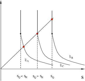
Figure 1: [Color online] Singularities of the isobaric partition (1) and the corresponding graphical solution of Eq. (9) which describes a PT in the models similar to QGBSTM. The solution of Eq. (9) is shown by a filled hexagon. $F(s,\xi)$ is shown by a solid curve for a few values of the parameter sets $\xi$. $F(s,\xi)$ diverges for $s<s_{Q}(\xi)$ (shown by dashed lines), but is finite at $s=s_{Q}(\xi)$ (shown by black circle). At low values of the parameters $\xi=\xi_{A}$, which can be either $\xi\equiv\{T,\mu=const\}$ or $\xi\equiv\{T=const,\mu\}$, the simple pole $s_{H}$ is the rightmost singularity and it corresponds to hadronic phase. For $\xi=\xi_{B}\gg\xi_{A}$ the rightmost singularity is an essential singularity $s=s_{Q}(\xi_{B})$, which describes QGP. At intermediate value $\xi=\xi_{C}$ both singularities coincide $s_{H}(\xi_{C})=s_{Q}(\xi_{C})$ and this condition is a Gibbs criterion (10). At transition from the low energy density phase to the high density one the rightmost singularity changes from the simple pole to the essential singularity.

III Conditions for the critical endpoint existence

Under adopted assumption the rightmost singularity in the QGBSTM2 is always the simple pole since in the right hand side vicinity of $s\rightarrow s_{Q}(T,\mu)+0$ the value of $F_{Q}(s,T,\mu)\rightarrow\infty$ for $\Sigma=\Sigma^{+}<0$. Then the motion of singularities corresponds to Fig. 2 in this situation. The question, however, appears whether such a behavior corresponds to PT. To clarify the point it is convenient to introduce the variable $\Delta^{\pm}\equiv\Delta(T_{\Sigma}\pm 0,\mu)=s^{\pm}-s_{Q}(T_{\Sigma}\pm 0,\mu)$ and to compare the $T$ derivative of the right most singularity $s^{-}\equiv s^{*}(T_{\Sigma}-0,\mu)$ below and $s^{+}\equiv s^{*}(T_{\Sigma}+0,\mu)$ above the PT line $T_{c}(\mu)=T_{\Sigma}(\mu)$ for the same magnitudes of $\mu$. Due to the relation between the system pressure $p(T,\mu)$ and the rightmost singularity $s^{*}(T,\mu)=\frac{p(T,\mu)}{T}$, the difference of $T$ derivatives, $\frac{\partial(\Delta^{+}-\Delta^{-})}{\partial~{}~{}T}$, if revealed on both sides of the PT line is defined by the difference of the corresponding entropy densities. Therefore, according to the standard classification of the PT order an appearance of nonzero values of $\frac{\partial(\Delta^{+}-\Delta^{-})}{\partial~{}~{}T}\neq 0$ signals about the 1^st order PT.

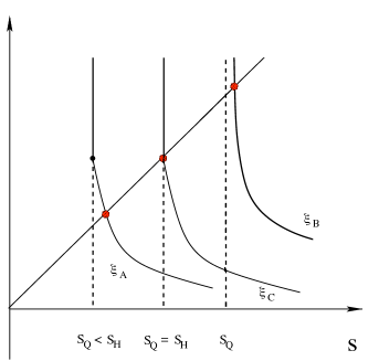
Figure 2: [Color online] Singularities of the isobaric partition (1) and the corresponding graphical solution of Eq. (9) which describes a PT in the QGBSTM2. The legend corresponds to Fig. 1. In this case, however, the rightmost singularity for each phase is the simple pole, whereas at the PT the essential singularity matches the simple pole due to the vanishing surface tension coefficient.

Now using the auxiliary functions

$${\cal K}_{a}\left(x\right) \equiv \int\limits_{V_{0}\Delta}^{\infty}dz~{}\frac{\exp\left[-z+xz^{\varkappa}\right]}{z^{a}}\,,$$ (11)

$$g_{\tau}(\Delta^{\pm},\Sigma^{\pm}) \equiv \frac{\exp\left[-\Delta^{\pm}V_{0}-\Sigma^{\pm}V_{0}^{\varkappa}\right]}{(\tau-1)\,V_{0}^{\tau-1}}\,,$$ (12)

it is possible to rewrite the continuous part of volume spectrum (3) as $F_{Q}(s^{\pm},T,\mu)={\textstyle u(T)}I_{\tau}(\Delta^{\pm},\Sigma^{\pm})$ integrating by parts the following integral

$$I_{\tau}(\Delta^{\pm},\Sigma^{\pm})\equiv\int\limits_{V_{0}}^{\infty}dv~{}\frac{\exp\left[-\Delta^{\pm}v-\Sigma^{\pm}v^{\varkappa}\right]}{v^{\tau}}=$$

$$\left[g_{\tau}(\Delta^{\pm},\Sigma^{\pm})-\frac{\Delta^{\pm}}{\tau-1}g_{\tau-1}(\Delta^{\pm},\Sigma^{\pm})\right.-$$

$$\frac{\varkappa\Sigma^{\pm}}{\tau-1}g_{\tau-\varkappa}(\Delta^{\pm},\Sigma^{\pm})+\left.\frac{(\Delta^{\pm})^{\tau-1}}{\tau-1}\Phi\left(-\frac{\Sigma^{\pm}}{(\Delta^{\pm})^{\varkappa}}\right)\right]\,,$$ (13)

$$\Phi(x)\equiv{\cal K}_{\tau-2}(x)-\frac{\varkappa(2\tau-3-\varkappa)\,x}{(\tau-2)(\tau-1-\varkappa)}{\cal K}_{\tau-1-\varkappa}(x)+$$

$$\frac{\varkappa^{2}\,x^{2}}{\tau-1-\varkappa}{\cal K}_{\tau-2\varkappa}(x)\,.$$ (14)

Drawing Eqs. (III) and (14) one can show the necessary condition of deconfinement PT existence at $\Sigma^{\pm}\rightarrow 0$ becomes $s_{Q}(T_{\Sigma},\mu)=F_{H}(s_{Q}(T_{\Sigma},\mu),T_{\Sigma},\mu)+u(T_{\Sigma})g_{\tau}(0,0)$ and it provides $\Delta^{\pm}\rightarrow+0$, indeed. For $\tau<1+2\varkappa$ such a statement follows directly from the present form of (14), whereas for larger values of $\tau$ exponent one needs to integrate ${\cal K}_{a}(x)$-functions in (14) while they converge at the lower integration limit for $\Delta^{\pm}\rightarrow+0$.

With treating Eqs. (11)-(14) one can easily find

$$\frac{\partial\Delta^{\pm}}{\partial~{}T}= \frac{\frac{\partial F_{H}}{\partial T}+\frac{\partial s_{Q}}{\partial T}\left[\frac{\partial F_{H}}{\partial s}-1\right]+\frac{\partial u}{\partial T}I_{\tau}(\Delta^{\pm},\Sigma^{\pm})}{1+uI_{\tau-1}(\Delta^{\pm},\Sigma^{\pm})-\frac{\partial F_{H}}{\partial s}}-$$

$$\frac{uI_{\tau-\varkappa}(\Delta^{\pm},\Sigma^{\pm})\frac{\partial\Sigma^{\pm}}{\partial T}}{1+uI_{\tau-1}(\Delta^{\pm},\Sigma^{\pm})-\frac{\partial F_{H}}{\partial s}}\,,$$ (15)

which in the limit $\Delta^{\pm},\Sigma^{\pm}\rightarrow 0$ gives

$$\frac{\partial\Delta^{+}}{\partial~{}T}-\frac{\partial\Delta^{-}}{\partial~{}T}\rightarrow -\frac{uI_{\tau-\varkappa}(0,0)\left[\frac{\partial\Sigma^{+}}{\partial T}-\frac{\partial\Sigma^{-}}{\partial T}\right]}{1+uI_{\tau-1}(0,0)-\frac{\partial F_{H}}{\partial s}}\,.$$ (16)

This is a remarkable result because it clearly shows in the present model the 1^st order deconfinement PT does exist, if the $T$ derivative of reduced surface tension coefficient has a discontinuity at the phase equilibrium line only! Thus, a discontinuity of the first derivative of a system pressure, which is a three-dimensional quantity, is generated by a discontinuity of the derivative of surface tension coefficient, which is a two-dimensional characteristics. In the other words, within the QGBSTM2 the deconfinement 1^st order PT is just a surface induced one. The necessary condition for its existence is the finiteness of integrals $I_{\tau-\varkappa}(0,0)$ and $I_{\tau-1}(0,0)$ in (16), i.e. $\tau>2$.

Moreover, to realize a PT from hadronic matter to QGP it is necessary to have at the PT line $\frac{\partial\Delta^{+}}{\partial~{}T}-\frac{\partial\Delta^{-}}{\partial~{}T}=\frac{1}{T}\frac{\partial}{\partial T}\left[p_{Q}(T,\mu)-p_{H}(T,\mu)\right]>0$ and, hence, at this line

$$\frac{\partial\Sigma^{+}}{\partial T}-\frac{\partial\Sigma^{-}}{\partial T}<0\,.$$ (17)

Now it is clear that at the critical endpoint $(\mu_{end};T_{c}(\mu_{end}))$ the entropy density gap vanishes due to the disappearing difference $\frac{\partial\Sigma^{+}}{\partial T}-\frac{\partial\Sigma^{-}}{\partial T}=0$.

With the general parameterization of reduced surface tension coefficient which is consistent with (8)

$$\Sigma(T,\mu)=\frac{1}{T}\cdot\left\{\begin{array}[]{rr}\sigma^{-}\left[\frac{T_{\Sigma}(\mu)-T}{T_{\Sigma}(\mu)}\right]^{\zeta^{-}}\,,&\hskip 2.84544ptT\rightarrow T_{\Sigma}(\mu)-0\,,\\ &\\ -\sigma^{+}\left[\frac{T-T_{\Sigma}(\mu)}{T_{\Sigma}(\mu)}\right]^{\zeta^{+}}\,,&\hskip 2.84544ptT\rightarrow T_{\Sigma}(\mu)+0\,,\end{array}\right.$$ (21)

we are able to conclude about the powers $\zeta^{\pm}$ and the values of coefficients $\sigma^{\pm}\geq 0$. It is obvious from (III) that $\zeta^{\pm}\geq 1$, otherwise the corresponding entropy density is divergent at the PT line. If, for instance, $\zeta^{+}=1$, as predicted by the Hills and Dales model Bugaev:04b , then $\zeta^{-}=1$, and according to (17) one has $\sigma^{+}>\sigma^{-}$. If, however, $\zeta^{-}>1$, then from (17) it follows that $\sigma^{+}\,\zeta^{+}(T-T_{\Sigma}(\mu))^{\zeta^{+}-1}>0$ for $T\rightarrow T_{\Sigma}(\mu)+0$. The latter is consistent with the equality $\zeta^{+}=1$.

It can be shown that in accordance with (10) the inequalities

$${\textstyle\frac{\partial F_{H}}{\partial T}+\frac{\partial s_{Q}}{\partial T}\left[\frac{\partial F_{H}}{\partial s}-1\right]+\frac{\partial u}{\partial T}g_{\tau}(0,0)\gtrless ug_{\tau-\varkappa}(0,0)\frac{\partial\Sigma^{\pm}}{\partial T}}$$ (22)

are the sufficient conditions of the 1^st order PT existence that provide (17) and guarantee the uniqueness of solutions $\Delta^{\pm}\rightarrow+0$ on both sides of the PT line.

The critical endpoint $(\mu_{end};T_{c}(\mu_{end}))$ exists, if in its vicinity the difference of coefficients $\sigma^{\pm}$ vanishes as

$$\sigma^{+}-\sigma^{-}\sim d^{\zeta_{end}},~{}~{}d\equiv T-T_{c}(\mu_{end})-\frac{\partial T_{\Sigma}}{\partial\mu}\biggl{|}_{\mu_{end}}(\mu-\mu_{end})$$ (23)

with $\zeta_{end}\geq 1$. By construction in the $\mu-T$ plane $d$ as defined by (23) vanishes at the tangent line to the PT curve at $(\mu_{end};T_{c}(\mu_{end}))$. As one can easily see from either $T$ or $\mu$ derivative of (III) any second derivative of the difference $\Delta^{+}-\Delta^{-}=0$ at the critical endpoint $(\mu_{end};T_{c}(\mu_{end}))$, if $\zeta^{+}=\zeta^{-}=\zeta_{end}=1$ only, which provides the 2^nd order PT available at this point. The higher order PT at the critical endpoint may exist for $\zeta_{end}=2$

IV Conclusion

Here we presented new exactly solvable model, QGBSTM2, (or even the class of models) which develops the critical endpoint at $(\mu_{end};T_{c}(\mu_{end}))$. This model naturally explains the transformation of the 1^st order deconfining PT into a weaker PT at the endpoint and into a cross-over at low baryonic densities as driven by negative surface tension coefficient of the QGP bags at high energy densities. It sheds new light on the QGP equation of state suggested in Ref.QGBSTM where it has been shown that the deconfined QGP phase presents itself just a single infinite bag whereas the cross-over phase consists of the QGP bags of all possible volumes and only at very high pressure values this phase is presented by one large (infinite) bag. The important consequence of such a property is that the deconfined QGP phase should be separated from the cross-over QGP by another PT which is induced by the change of surface tension coefficient sign of large bags. Furthermore, QGBSTM teaches us that for the Fisher exponent the 1^st order deconfinement PT exists for $1<\tau\leq 2$ only, whereas at the endpoint there exists the 2^nd order PT for $\frac{3}{2}<\tau\leq 2$ and this point is the tri-critical one.

On the other hand the important message of QGBSTM2 is that a solvable model of the QCD critical endpoint can be formulated for $\tau>2$. Technically it is achieved by matching the deconfinement PT line with the line of vanishing surface tension coefficient $T_{\Sigma}(\mu)$ for $\mu\geq\mu_{end}$ and $T\leq T_{c}(\mu_{end})$. This step leads to new strong assertion that the 1^st order PT in QGBSTM2 is not accompanied by change of the leading singularity type as was argued earlier in Refs. CGreiner:06 ; Bugaev:05c . Thus, the high density QGP phase is defined by not an essential singularity of the isobaric partition (1) but its simple pole. Similar to QGBSTM the high density phase of this model is defined by the QGP crossover whereas the deconfined matter (an interior of single infinite bag) may exist at the mixed phase inherent in the deconfinement PT only. Besides we find also that the 1^st order deconfining PT, i.e. a discontinuity of the first derivative of a system pressure, which is a three-dimensional quantity, is generated by the discontinuity of surface tension coefficient derivative, which is a two-dimensional quantity. Thus, we explicitly show that within the present model the deconfinement 1^st order PT is the surface induced one.
Another distinctive feature of these results is that for the first time we see the critical endpoint in the model with the constituents of nonzero proper volume exists not for $\tau\leq 1$ as in the SMM simpleSMM:1 ; Bugaev:00 and not for $1<\tau\leq 2$ as the tricritical endpoints in the SMM and in the QGBSTM QGBSTM , but for $\tau>2$, i.e. as in FDM Fisher:67 . Perhaps, this feature may be helpful to distinguish experimentally the QCD critical endpoint from the tri-critical one.

References

- (1) Z. Fodor, PoS Lattice 2007, 011 (2007).
- (2) F. Karsch, Prog. Theor. Phys. Suppl. 168, 237 (2007).
- (3) P. de Forcrand and O. Philipsen, PoS Lattice 2008; arXiv:0811.3858 [hep-lat]; arXiv:0807.0860 [hep-lat].
- (4) for more references see K. Wilson and J. Kogut, Phys. Rep. 12, 75 (1974).
- (5) M. E. Fisher, Physics 3, 255 (1967).
- (6) for a review on Fisher scaling see J. B. Elliott, K. A. Bugaev, L. G. Moretto and L. Phair, arXiv:nucl-ex/0608022 (2006) 36 p. and references therein.
- (7) L. G. Moretto et. al., Phys. Rep. 287, 249 (1997).
- (8) A. Dillmann and G. E. A. Meier, J. Chem. Phys. 94, 3872 (1991).
- (9) C. S. Kiang, Phys. Rev. Lett. 24, 47 (1970).
- (10) C. M. Mader et al., Phys. Rev. C 68, 064601 (2003).
- (11) L. G. Moretto et al., Phys. Rev. Lett. 94, 202701 (2005).
- (12) D. Stauffer and A. Aharony, “Introduction to Percolation”, Taylor and Francis, Philadelphia (2001).
- (13) J. P. Bondorf et al., Phys. Rep. 257, 131 (1995).
- (14) S. Das Gupta and A.Z. Mekjian, Phys. Rev. C 57, 1361 (1998).
- (15) K. A. Bugaev, M. I. Gorenstein, I. N. Mishustin and W. Greiner, Phys. Rev. C62, 044320 (2000); arXiv:nucl-th/0007062 (2000); Phys. Lett. B 498, 144 (2001); arXiv:nucl-th/0103075 (2001).
- (16) P. T. Reuter and K. A. Bugaev, Phys. Lett. B 517, 233 (2001).
- (17) Y. Aoki et al., Nature 443 (2006) 675; arXiv:hep-lat/0611014.
- (18) R. D. Pisarski and F. Wilczek, Phys. Rev. D 29, 338 (1984).
- (19) M. Stephanov, PoS LAT2006:024, ( 2006).
- (20) A.Di Giacomo, arXiv:0901.0227 [hep-lat].
- (21) for more references see U. Heller, PoS LAT2006:011, (2006); K. Szabo, PoS LAT2006:149 (2006).
- (22) E. V. Shuryak, arXiv:0807.3033 [hep-ph].
- (23) see, for instance, A. Karch et al., Phys. Rev. D 74, 015005 (2006).
- (24) K. A. Bugaev, Phys. Rev. C 76, 014903 (2007).
- (25) K. A. Bugaev, Physics of Atomic Nuclei, 71, 1615 (2008).
- (26) K. A. Bugaev, V. K. Petrov and G. M. Zinovjev, Europhys. Lett. 85, 22002 (2009); arXiv:0801.4869 [hep-ph]; arXiv:0807.2391 [hep-ph].
- (27) see, for instance, M. I. Gorenstein, M. Gaździcki and W. Greiner, Phys. Rev. C 72, 024909 (2005); N. G. Antoniou, F. K. Diakonos and A. S. Kapoyannis, Nucl. Phys. A 759, 417 (2005) and references therein.
- (28) C. Nonaka and M. Asakawa, Phys. Rev. C 71, 044904 (2005).
- (29) for the list of references see I. Zakout, C. Greiner, J. Schaffner-Bielich, Nucl. Phys. A 781, 150 (2007).
- (30) K. A. Bugaev, Phys. Part. Nucl. 38, (2007) 447.
- (31) R. Hagedorn, Nuovo Cimento Suppl. 3, 147 (1965).
- (32) J. I. Kapusta, Phys. Rev. D 23, 2444 (1981).
- (33) K. A. Bugaev, L. Phair and J. B. Elliott, Phys. Rev. E 72, 047106 (2005); K. A. Bugaev and J. B. Elliott, Ukr. J. Phys. 52 (2007) 301.
- (34) for a discussion see K. A. Bugaev, arXiv:0809.1023 [nucl-th].