Influence on observation from IR divergence during inflation
— Multi field inflation —

Abstract

We propose one way to regularize the fluctuations generated during inflation, whose infrared (IR) corrections diverge logarithmically. In the case of a single field inflation model, recently, we proposed one solution to the IR divergence problem. There, we introduced new perturbative variables which better mimic actual observable fluctuations, and proved the regularity of correlation functions with respect to these variables. In this paper, we extend our previous discussions to a multi field inflation model. We show that, as long as we consider the case that the non-linear interaction acts for a finite duration, observable fluctuations are free from IR divergences in the multi field model, too. In contrast to the single field model, to discuss observables, we need to take into account the effects of quantum decoherence which pick up a unique history of the universe from various possibilities contained in initial quantum state set naturally in the early stage of the universe.

I Introduction

It is widely known that on the computation of the non-linear perturbations generated during inflation we encounter the divergence coming from the infrared (IR) corrections  Boyanovsky:2004gq ; Boyanovsky:2004ph ; Boyanovsky:2005sh ; Boyanovsky:2005px ; Onemli:2002hr ; Brunier:2004sb ; Prokopec:2007ak ; Sloth:2006az ; Sloth:2006nu ; Seery:2007we ; Seery:2007wf ; Urakawa:2008rb . As the possibility of detecting the non-linear primordial perturbations is increasing  Komatsu:2008hk Bartolo:2001cw ; Bartolo:2004if ; Maldacena:2002vr ; Kim:2006te ; Babich:2004gb ; Seery:2005wm ; Seery:2005gb ; Weinberg:2005vy ; Weinberg:2006ac ; Rigopoulos:2005xx ; Rigopoulos:2005ae ; Rigopoulos:2005us ; Vernizzi:2006ve ; Chen:2006nt ; Battefeld:2006sz ; Yokoyama:2007dw ; Yokoyama:2008by ; Seery:2008ax ; Naruko:2008sq ; Weinberg:2008mc ; Weinberg:2008nf ; Weinberg:2008si ; Cogollo:2008bi ; Rodriguez:2008hy , it becomes more important to solve the IR divergence problem for the primordial perturbations and to predict their finite amplitude that we observe Lyth:2007jh ; Bartolo:2007ti ; Riotto:2008mv ; Enqvist:2008kt ; Urakawa:2009my . In our previous work Urakawa:2009my , we have proposed one way to solve this IR divergence problem in the single-field inflation model. The key observation is that the variables that are commonly used in describing fluctuations are influenced by what we cannot observe. This is because we can observe only the fluctuations within the region causally connected to us. We usually define the fluctuation by the deviation from the background value which is the spatial average over the whole universe. However, since we can observe only a finite volume of the universe, the fluctuations evaluated in such a way are inevitably influenced by the information contained in the unobservable region. In general, the deviation from the global average is much larger than the deviation from the local average, which leads to the over-estimation of the fluctuations due to the contribution from long wavelength fluctuations. In addition to that, to discuss the so-called observable quantities in the framework of the standard cosmological perturbation (even though people call it gauge invariant formulation), in practice it is necessary to fix the gauge, say, the flat gauge. As long as the gauge is determined by solving elliptic-type equations on each constant time slice, the gauge choice is inevitably affected by the information in the region causally disconnected to us. Gauge dependence of the perturbation variables itself is not a problem since the “true observables” such as the statistical property of the sky map of the temperature fluctuation of the cosmic microwave background are not affected by the gauge choice. However, if divergences appear in the quantities computed at the intermediate steps such as $n$-point functions of the perturbation fields, it becomes almost impossible to extract information about the “true observables” from them.

To shut off the influence from the unobservable region of the universe, we focused on the presence of residual gauge degrees of freedom in flat gauge. To remove the harmful part in the residual gauge degrees of freedom, we imposed a further gauge condition which insists the local average of the inflaton to vanish. Then, the fluctuation is not influenced by the information from the causally disconnected region. We gave a proof that IR divergences are absent in this new scheme. In this paper, we extend our discussion to the multi-field models. Since the adjustment of the average value is possible only for one field, even if we adopt the local gauge, the fluctuations of the other components of the scalar fields $\varphi^{I}$ are still influenced by the causally disconnected region. Here we denote the index for the D-component scalar fields by $I=1,\cdots,D$. Reflecting this fact, when plural fields are associated with the IR divergences, the prescription presented in our previous paper Urakawa:2009my is not enough to regularize IR divergences. To remove the influence from what we cannot observe, we introduce new perturbation variables from which we can compute the “true observables”. As the new variables, we consider the local perturbations of the fields defined by the deviation from their local average values. Then, we prove the regularity of $n$-point functions of these new variables.

We should note that $n$-point functions for the local perturbations are still influenced by what we cannot observe. This is due to the difference between the quantum state of the universe which we set as a natural initial condition and the one which we observe in our real universe. The natural wave function of the inflationary universe is not peaked at a specific point in the space of the local average values of $\varphi^{I}$. At the observation time, this “natural” state of the universe can be decomposed into a superposition of wave packets which have a peak at a certain point. As the universe evolves, constituent wave packets lose correlation to each other. Through this so-called decoherence process, the coherent superposition of the wave packets starts to behave as a statistical ensemble of many different worlds, where each world means the universe described by a decohered wave packet Polarski:1995jg ; Kiefer:2006je ; Starobinsky:1986fx . Our observed world is just a representative one expressed by a wave packet randomly chosen from the various possibilities. Once we select one wave packet after the decoherence occurs, the evolution of our world will not be affected by the other parallel worlds. However, the initial quantum state does include the contributions from all the wave packets. This implies that a naive computation of $n$-point functions is contaminated by the other worlds uncorrelated to ours. In this paper, taking into account the decoherence of the quantum state of the universe, we propose a way to define “observables” and show that they are actually finite without suffering from IR divergence.

However, to be honest, the “observables” that we introduce do not correspond exactly to what we measure in the actual observations. Not to mislead the reader, we should stress here that our definition of “observables” does not respect the aspect explained in the preceding paragraph in a completely satisfactory manner. They are not the expectation values for a single decohered wave packet. What we define is not completely free from the contamination of the other worlds decohered from ours. However, since we define our “observables” so as to over-estimate the amplitude of fluctuations, the proof of their finiteness ensures the finiteness of what we really observe. Recently the stochastic approach  Starobinsky:1986fx ; Starobinsky:1994bd has been employed in order to solve the IR divergence problem Bartolo:2007ti ; Riotto:2008mv ; Enqvist:2008kt . This is in harmony with our claim. In stochastic approach, we assume that the modes that exceed a certain length scale are automatically decohered Starobinsky:1986fx ; Starobinsky:1994bd ; Nakao:1988yi ; Nambu:1988je ; Morikawa:1989xz ; Morikawa:1987ci ; Tanaka:1997iy ; Seery:2009hs . Namely, long-wavelength fluctuations are treated as the statistical variance. Since our unique “world” is one realization in this statistical ensemble, there is no contribution to the observed quantum fluctuations from long-wavelength modes by definition. This is a practical way to take into account the quantum decoherence in the inflationary universe, but this scheme cannot completely remove the artificial IR cut-off scale from the discussion. Moreover, it is hard to deny the spiteful criticism that the reason why the problem of IR divergence does not appear in the stochastic approach might be simply because quantum fluctuations in the IR limit are neglected by hand. In contrast, in our approach, to avoid under-estimating the amplitude of fluctuations, we accepted small contamination from the other parallel worlds, which will make the amplitude of fluctuations larger. Namely, sacrificing the accuracy of the estimate of the amplitude of fluctuations, we choose to show the IR regularity of the observables by over-estimating the amplitude of fluctuations.

This paper is organised as follows. In Sec. II, we give the set up of our problems. Following it, we propose a prescription to define “observables”. The basic idea of our proposal that assures the IR regularity is stated in this section. In Sec. III we explain the details of the proof of IR regularity In Sec. IV, we summarize our results. On the computation of the non-linear corrections, the both integrations over the temporal and spatial coordinates can make IR corrections singular. In this paper, maintaining the initial time $t_{i}$ at a finite past, we restrict ourselves to the time evolution of perturbations for a finite period of time during inflation. In Sec. IV, we add the comments on the case in which we send $t_{i}$ to distant past.

II A Solution to IR problem

II.1 Setup of the problem

We first define the setup of the problem that we study in this paper. We consider the multi-component inflation model with the conventional kinetic term. The total action is given by

$$S=\frac{1}{2}\int\sqrt{-g}~{}[M_{\rm pl}^{2}R-{\cal G}_{IJ}g^{\mu\nu}\Phi^{I}_{,\mu}\Phi^{J}_{,\nu}-2U(\Phi)]d^{4}x~{},$$

where $M_{\rm pl}$ is the Planck mass. We denote the field-space metric by ${\cal G}_{IJ}$. For simplicity, we assume ${\cal G}_{IJ}$ is a constant matrix. We perform the following change of variables

$$\phi_{I}\equiv\Phi_{I}/M_{\rm pl},\quad V(\phi)\equiv U(\Phi)/M_{\rm pl}^{2},$$ (2)

to factorize $M_{\rm pl}^{2}$ from the action as

$$S=\frac{M_{\rm pl}^{2}}{2}\int\sqrt{-g}~{}[R-g^{\mu\nu}\phi_{I,\mu}\phi^{I}_{,\nu}-2V(\phi)]d^{4}x~{},$$ (3)

where $\phi_{I}\equiv{\cal G}_{IJ}\phi^{I}$. Since the Planck mass is completely factored out, the equations of motion do not depend on it. The Planck mass appears only in the amplitude of quantum fluctuation. Namely, the typical amplitude of fluctuation of $\Phi^{I}$ is $H$, and hence that of $\phi^{I}$ is $H/M_{\rm pl}$.

In order to discuss the nonlinearity, it is convenient to use the ADM formalism Maldacena:2002vr ; Seery:2005wm ; Seery:2005gb , where the line element is expressed in terms of the lapse function $N$, the shift vector $N^{a}$, and the spatial metric $h_{ab}$:

$$ds^{2}=-N^{2}dt^{2}+h_{ab}(dx^{a}+N^{a}dt)(dx^{b}+N^{b}dt)~{}.$$ (4)

Substituting this metric form, we can denote the action as

$$S \!\!= \!\!\frac{M_{\rm pl}^{2}}{2}\int\sqrt{h}\Bigl{[}N\,^{(3)}\!R-2NV(\phi)+\frac{1}{N}(E_{ab}E^{ab}-E^{2})$$ (7)

$$\qquad\qquad\quad+~{}\frac{1}{N}(\dot{\phi}_{I}-N^{a}\partial_{a}\phi_{I})(\dot{\phi}^{I}-N^{a}\partial_{a}\phi^{I})$$

$$\qquad\qquad\quad-~{}Nh^{ab}\partial_{a}\phi_{I}\partial_{b}\phi^{I}\Bigr{]}d^{4}x~{},$$

where

$$E_{ab}=\frac{1}{2}\{\dot{h}_{ab}-D_{a}N_{b}-D_{b}N_{a}\}~{},$$ (8)

$$E=h^{ab}E_{ab}~{},$$ (9)

and $D$ is the covariant differentiation associated with $h_{ab}$. A dot “ $\dot{~{}}$ ” represents a differentiation with respect the time coordinate. In the ADM formalism, we can obtain the constraint equations easily by varying the action with respect to $N$ and $N^{a}$, which play the role of Lagrange multipliers. We obtain the Hamiltonian constraint equation and the momentum constraint equations as

$${}^{(3)}R-2V-N^{-2}(E^{ab}E_{ab}-E^{2})$$ (10)

$$\qquad-~{}N^{-2}(\dot{\phi}^{I}-N^{a}\partial_{a}\phi^{I})(\dot{\phi}_{I}-N^{a}\partial_{a}\phi_{I})$$ (11)

$$\qquad-~{}h^{ab}\partial_{a}\phi^{I}\partial_{b}\phi_{I}=0~{},$$ (12)

$$D_{a}[N^{-1}(E^{a}_{~{}b}-\delta^{a}_{~{}b}E)]-N^{-1}\partial_{b}\phi_{I}(\dot{\phi}^{I}-N^{a}\partial_{a}\phi^{I})=0~{}.$$

Hereafter, neglecting the vector perturbation, we denote the shift vector as $N_{a}=\partial_{a}\chi$. In this paper we work in the flat gauge, defined by

$$h_{ab}=e^{2\rho}\delta_{ab}~{},$$ (14)

where $a\equiv e^{\rho}$ is the background scale factor. Here we have also neglected the tensor perturbation, focusing only on the scalar perturbation, in which the IR divergence of our interest arises Boyanovsky:2005px ; Urakawa:2008rb .

In this gauge, using $N$, $\chi$ and the fluctuation of the scalar fields $\varphi^{I}$, the total action is written as

$$S \!= \!\frac{M_{\rm pl}^{2}}{2}\int dt\,d^{3}\!{\bm{x}}\,e^{3\rho}\Bigl{[}-2N~{}\displaystyle\sum_{n=0}\frac{1}{n!}V_{I_{1}\cdots I_{n}}(\phi)\varphi^{I_{1}}\cdots\varphi^{I_{n}}$$ (15)

$$~{}+N^{-1}\{-6\dot{\rho}^{2}+4\dot{\rho}~{}\triangle\chi$$

$$\qquad\qquad\qquad\qquad+(\nabla^{a}\nabla^{b}\chi\nabla_{a}\nabla_{b}\chi-(\triangle\chi)^{2})\}$$

$$~{}+N^{-1}(\dot{\phi}^{I}+\dot{\varphi}^{I}-\nabla^{a}\chi\nabla_{a}\varphi^{I})(\dot{\phi}_{I}+\dot{\varphi}_{I}-\nabla^{a}\chi\nabla_{a}\varphi_{I})$$

$$\qquad\qquad\qquad\qquad-N\nabla_{a}\varphi_{I}\nabla^{a}\varphi^{I}\Bigr{]}~{},$$

and two constraint equations are

$$2N^{2}\displaystyle\sum_{n=0}\frac{1}{n!}V_{I_{1}\cdots I_{n}}(\phi)\varphi^{I_{1}}\cdots\varphi^{I_{n}}-6\dot{\rho}^{2}$$ (16)

$$\qquad+~{}4\dot{\rho}\triangle\chi+\{\nabla^{a}\nabla^{b}\chi\nabla_{a}\nabla_{b}\chi-(\triangle\chi)^{2}\}$$ (17)

$$\qquad+~{}(\dot{\phi}_{I}+\dot{\varphi}_{I}-\nabla^{a}\chi\nabla_{a}\varphi_{I})(\dot{\phi}^{I}+\dot{\varphi}^{I}-\nabla^{b}\chi\nabla_{b}\varphi^{I})$$ (18)

$$\qquad+~{}N^{2}\nabla_{a}\varphi_{I}\nabla^{a}\varphi^{I}=0,$$

(19)

$$(\nabla_{a}N)\{2\dot{\rho}\delta^{a}_{~{}b}+(\nabla^{a}\nabla_{b}\chi-\delta^{a}_{~{}b}\triangle\chi)\}$$ (20)

$$\qquad-(\nabla_{b}\varphi_{I})N~{}(\dot{\phi}^{I}+\dot{\varphi}^{I}-\nabla^{a}\chi\nabla_{a}\varphi^{I})=0~{},$$

where

$$\nabla_{a}\equiv e^{-\rho}\partial_{a}~{},$$

represents the three dimensional partial differentiation with respect to the proper length coordinates ${\bm{X}}\equiv e^{\rho}{\bm{x}}$ and

$$\triangle\equiv\delta^{ab}\nabla_{a}\nabla_{b}~{}.$$

Spatial indices, $a,b,\cdots$, are raised by $\delta^{ab}$. We use this notation, which respects the proper distance, because it eliminates all the complicated scale factor dependences from the action. We define the derivatives of the potential as

$$V_{I_{1}I_{2}\cdots I_{n}}(\phi)\equiv\frac{\partial^{n}V(\phi)}{\partial\phi^{I_{1}}\partial\phi^{I_{2}}\cdots\partial\phi^{I_{n}}}~{}.$$ (22)

The background quantities $\rho$ and $\phi$ satisfy the following equations :

$$3\dot{\rho}^{2}=\frac{1}{2}\dot{\phi}^{I}\dot{\phi}_{I}+V(\phi)~{},$$ (23)

$$\ddot{\phi}^{I}+3\dot{\rho}\dot{\phi}^{I}+V^{I}=0~{},$$ (24)

$$\ddot{\rho}=-\frac{1}{2}\dot{\phi}^{I}\dot{\phi}_{I}~{}.$$ (25)

Expanding the variables as

$$N = 1+\delta N_{1}+\frac{1}{2}\delta N_{2}+\cdots~{},$$

$$\chi = \chi_{1}+\frac{1}{2}\chi_{2}+\cdots~{},$$

$$\varphi^{I} = \varphi^{I}_{1}+\frac{1}{2}\varphi^{I}_{2}+\cdots~{},$$

we find that the first order constraint equations are

$$V_{I}\varphi_{1}^{I}+2V\delta N_{1}+2\dot{\rho}\triangle^{2}\chi_{1}~{},+\dot{\phi}_{I}\dot{\varphi}^{I}_{1}=0~{},$$ (26)

$$\nabla_{a}\left(2\dot{\rho}~{}\delta N_{1}-\dot{\phi}_{I}\varphi^{I}_{1}\right)=0~{}.$$ (27)

The first order perturbation $\varphi^{I}_{1}$ is identified with the field perturbation in the interaction picture. Taking the deviation of the action with respect to $\varphi_{I}$, we can derive the equation of motion for $\varphi_{I}$, which includes the Lagrange multipliers $\delta N$ and $\chi$. For example, from the third order action, we can derive the equation of motion with quadratic interaction terms as follows,

$$\ddot{\varphi}^{I}+3\dot{\rho}\dot{\varphi}^{I}-\triangle\varphi^{I}+V^{I}_{\,J}\varphi^{J}-\dot{\phi}^{I}\triangle\chi+\delta NV^{I}-3\dot{\rho}~{}\dot{\phi}^{I}\delta N-\partial_{t}(\delta N\dot{\phi}^{I})$$

$$\qquad+~{}\frac{1}{2}V^{I}_{\,JK}\varphi^{J}\varphi^{K}-\nabla_{a}(\dot{\varphi}^{I}-\dot{\phi}^{I}\delta N)\nabla^{a}\chi-(\dot{\varphi}^{I}-\dot{\phi}^{I}\delta N)\triangle^{2}\chi-\dot{\rho}\nabla^{a}\chi\nabla_{a}\varphi^{I}-\partial_{t}(\nabla^{a}\chi\nabla_{a}\varphi^{I})$$

$$\qquad-~{}3\dot{\rho}~{}\dot{\varphi}^{I}\delta N-\partial_{t}(\delta N\dot{\varphi}^{I})-\nabla_{a}(\delta N\nabla^{a}\varphi^{I})+V^{I}_{\,J}\varphi^{J}\delta N+3\dot{\rho}\dot{\phi}^{I}\delta N^{2}+\partial_{t}(\dot{\phi}^{I}\delta N^{2})=0$$

(28)

Solving the constraint equations at each order, we can express the lapse function and the shift vector as functions of $\varphi^{I}$ at lower order. Substituting these expressions into the equation of motion for $\varphi^{I}$, which is up to third order given by Eq. (28), the equation is written solely in terms of the dynamical degree of freedom, $\varphi^{I}$.

II.2 Tree-shaped graphs

In this subsection, as a preparation for computing $n$-point functions of $\varphi_{I}(x)$, we consider an expansion of the Heisenberg field $\varphi_{I}(x)$ in terms of the interaction picture field, using the retarded Green function $G_{{\rm R}}{}^{\!I}_{J}(x,x^{\prime})$, which is causal. Since the retarded Green function $G_{{\rm R}}{}^{\!I}_{J}(x,x^{\prime})$ has a finite non-vanishing support for fixed $x$ and $t^{\prime}$, its three dimensional Fourier transform with respect to $\bm{x}^{\prime}$ becomes regular in the IR limit.

Let us denote the equation of motion for $\varphi^{I}$ schematically by

$${\cal L}^{I}_{\,J}\varphi^{J}=-\Gamma^{I}[\varphi]~{},$$ (29)

where ${\cal L}^{I}_{\,J}$ is a second order differential operator corresponding to the linearized equation for $\varphi^{J}$ (Eq. (41)) and $\Gamma^{I}$ stands for all the nonlinear interaction terms. Using the retarded Green function $G_{{\rm R}}{}^{\!J}_{K}(x,x^{\prime})$ that satisfies

$${\cal L}^{I}_{\,J}G_{{\rm R}}{}^{\!J}_{K}(x,x^{\prime})=-a^{-3}\delta^{4}(x-x^{\prime})\delta^{I}_{\,K}~{},$$ (30)

we can solve Eq. (29) formally as

$$\!\!\varphi^{I}(x)=\varphi^{I}_{1}(x)+\int d^{4}\!x^{\prime}\,G_{{\rm R}}{}^{\!I}_{J}(x,x^{\prime})a^{3}(t^{\prime})\Gamma^{J}[\varphi](x^{\prime}).$$ (31)

where the first order perturbation $\varphi^{I}_{1}$ satisfies

$${\cal L}^{I}_{\,J}\varphi^{J}_{1}(x)=0~{}.$$ (32)

Here the factor $a^{3}$ originates from the background value of $\sqrt{-g}$. Substituting the expression (31) for $\varphi^{I}(x)$ iteratively into $\Gamma_{I}[\varphi]$ on its r.h.s., we obtain the Heisenberg field $\varphi^{I}(x)$ expanded in terms of $\varphi^{I}_{1}(x)$ to an arbitrary high order using the retarded Green function $G_{{\rm R}}{}^{\!I}_{J}(x,x^{\prime})$. As we have shown in Urakawa:2009my , to expand $\varphi^{I}$, a diagrammatic illustration will be useful. The Heisenberg field can be expressed by a summation of tree-shaped graphs in which all the retarded Green functions $G_{{\rm R}}{}^{\!I}_{J}(x,x^{\prime})$ are followed by two or more $\varphi^{I}_{1}(x^{\prime})$ or $G_{{\rm R}}{}^{\!I}_{J}(x^{\prime},x^{\prime\prime})$ with some integro-differential operators and all the interaction picture fields $\varphi^{I}_{1}(x)$ are located at the right most ends of the graphs.

When we compute the expectation value for $n$-point functions of the Heisenberg field, the interaction picture fields $\varphi_{I}$ in the tree-shaped graphs are contracted with each other to make pairs, which are replaced with Wightman functions, $G_{+}^{IJ}(x,x^{\prime})\equiv\langle\varphi^{I}_{1}(x)\varphi^{J}_{1}(x^{\prime})\rangle$ or $G_{-}^{IJ}(x,x^{\prime})(=G_{+}^{JI}(x^{\prime},x))$. These propagators are IR singular ($\propto 1/k^{3}$), which is the possible origin of IR divergences in momentum integrations. While, the retarded Green function

$$G_{{\rm R}}{}^{\!I}_{J}(x,x^{\prime})=i\theta(t-t^{\prime})M^{2}_{\rm pl}\{G^{~{}~{}I}_{+\,J}(x,x^{\prime})-G^{~{}~{}I}_{-\,J}(x,x^{\prime})\}~{},$$ (33)

(34)

is regular in the IR limit.

II.3 Iteration scheme and local gauge conditions

In our previous paper Urakawa:2009my , we have shown that the flat gauge still has residual gauge degrees of freedom. For instance, we can introduce an arbitrary function $f_{n}(t)$ to the $n$-th order lapse function and the shift vector as

$$\delta N_{n}~{}\rightarrow~{}\delta N_{n}+f_{n}(t),\quad\chi_{n}~{}\rightarrow~{}\chi_{n}-\frac{V}{6\dot{\rho}}X_{a}X^{a}f_{n}(t).$$

This gauge degree of freedom corresponds to the scale transformation. As is mentioned in § I, our final goal is to define finite observable quantities in place of the naively divergent quantum correlation functions. For this purpose, we need to define gauge invariant variables without the information contained in the region far outside ${\cal O}$. Then, we have to fix the residual gauge only using the information near the observable region ${\cal O}$.

In the multi-field model, it is convenient to decompose the perturbation into the adiabatic one, which is tangential to the background trajectory, and the entropy one, which is orthogonal to the background trajectory Gordon:2000hv . Using the residual gauge degrees of freedom, we fix the homogeneous mode in the direction of the background trajectory $e_{I}\equiv\dot{\phi}_{I}/(\dot{\phi}_{J}\dot{\phi}^{J})^{\frac{1}{2}}$ as

$$\hat{W}_{t}~{}e_{I}\tilde{\varphi}^{I}(t)\equiv\frac{1}{L_{t}^{3}}\int d^{3}\bm{x}~{}W_{t}(\bm{x})~{}e_{I}\tilde{\varphi}^{I}(t,~{}\bm{x})=0,$$ (35)

where $W_{t}(\bm{x})$ is a window function, which is unity in the finite region ${\cal O}_{t}\equiv{\cal O}\cap\Sigma_{t}$ with a rapidly vanishing halo in the surrounding region, where $\Sigma_{t}$ means a $t=$const. hypersurface corresponding to the time $t$. For definiteness, we introduce ${\cal O}^{\prime}_{t_{f}}\supset{\cal O}_{t_{f}}$ and define ${\cal O}^{\prime}$ as the causal past of ${\cal O}^{\prime}_{t_{f}}$. We require $W_{t}(\bm{x})$ to vanish in the region outside ${\cal O}^{\prime}$. In addition, $W_{t}(\bm{x})$ is supposed to be a sufficiently smooth function so that an artificial UV contribution is not induced by a sharp cutoff. $L_{t}$, an approximate radius of the region ${\cal O}_{t}$, is defined such that the normalization condition

$$\hat{W}_{t}1=1~{},$$

is satisfied.

We associated “$\,~{}\tilde{}~{}\,$” with the variables in the particular gauge satisfying Eq. (35), in order to clearly distinguish them from the variables for which the additional gauge condition is not imposed. The difference between the variables with and without “$\,~{}\tilde{}~{}\,$” is only in the boundary conditions. Hence, they obey the same differential equations, (27)-(28).

In order to fix the arbitrary functions $f_{n}(t)$ ($n=1,2,3,4,\cdots$) so as to satisfy the gauge condition (35), we need to obtain a formal solution for $\tilde{\varphi}$. The higher order lapse functions are determined by solving the momentum constraint given in the form

$$\nabla_{a}\left(\delta\tilde{N}_{n}-{1\over 2\dot{\rho}}\dot{\phi}_{I}\varphi^{I}_{n}\right)=\Xi^{(n)}_{a},\quad(n=1,2,3,\cdots),~{}$$ (36)

where the r.h.s. is the $n$-th order nonlinear term expressed in terms of the lower order lapse functions, shift vectors, and $\tilde{\varphi}$. As we neglect the vector perturbation, we consider only the scalar part of these equations, i.e. its divergence, which is formally solved as

$$\delta\tilde{N}_{n}=\delta\breve{N}_{n}+f_{n},$$ (37)

with

$$\delta\breve{N}_{n}={1\over 2\dot{\rho}}\dot{\phi}_{I}\varphi^{I}_{n}+\triangle^{-1}\nabla^{a}\Xi^{(n)}_{a}.$$

We define the operation $\triangle^{-1}$ by

$$\triangle^{-1}F(x)=-\frac{1}{4\pi}\int\frac{W_{t}(e^{-\rho}{\bm{Y}})d^{3}{\bm{Y}}}{|{\bm{X}}-{\bm{Y}}|}F(t,e^{-\rho}{\bm{Y}})~{},$$ (38)

so that it is completely determined by the local information in the neighborhood of ${\cal O}_{t}$. Similarly, the higher order shift vectors satisfy the Hamiltonian constraint in the form

$$\triangle\tilde{\chi}_{n}\! =\! {1\over 2}\left[{\ddot{\phi}_{I}}\,\varphi^{I}_{n}-{\dot{\phi}_{I}\over\dot{\rho}^{2}}\partial_{t}\left({\dot{\rho}\varphi^{I}_{n}}\right)\right]$$

$$\qquad\qquad-{V\over\dot{\rho}}\left(f_{n}+\triangle^{-1}\nabla^{a}\Xi^{(n)}_{a}\right)+C_{n},$$

where $C_{n}$ on the r.h.s. is a function expressed in terms of the lower order lapse functions, shift vector and $\tilde{\varphi}^{I}$. A formal solution for $\tilde{\chi}_{n}$ is given by

$$\tilde{\chi}_{n} \!\!= \!\!\breve{\chi}_{n}-{r^{2}V\over 6\dot{\rho}}f_{n}~{},$$ (39)

with

$$\breve{\chi}_{n} = \triangle^{-1}\Biggl{(}{1\over 2}\left[{\ddot{\phi}_{I}}\,\varphi^{I}_{n}-{\dot{\phi}_{I}\over\dot{\rho}^{2}}\partial_{t}\left({\dot{\rho}\varphi^{I}_{n}}\right)\right]$$

$$\qquad\qquad\qquad\qquad-{V\over\dot{\rho}}\triangle^{-1}\left(\nabla^{a}\Xi^{(n)}_{a}\right)+C_{n}\Biggr{)}~{}.$$

Substituting the expressions for the lapse function (37) and the shift vector (39) into the equation of motion for $\tilde{\varphi}$ truncated at the $n$-th order, we obtain an equation

$${\cal L}^{I}_{\,J}~{}\tilde{\varphi}^{J}_{n}-\dot{\phi}^{I}\dot{f}_{n}+\left({V\dot{\phi}^{I}\over\dot{\rho}}+2V^{I}\right)f_{n}=-W_{t}({\bm{x}})\Gamma^{I}_{n},$$ (40)

where, for later convenience, we have inserted a window function $W_{t}({\bm{x}})$ on the r.h.s., which does not alter the evolution in ${\cal O}$. The explicit form of ${\cal L}^{I}_{\,J}$ is given by

$${\cal L}^{I}_{\,J}\equiv(\partial^{2}_{t}+3\dot{\rho}\,\partial_{t}-\triangle)\delta^{I}_{\,J}+\left(V^{I}_{\,J}-e^{-3\rho}\dot{A}^{I}_{J}\right).$$ (41)

with

$$A^{I}_{J}(t)\equiv e^{3\rho}\dot{\phi}^{I}\dot{\phi}_{J}/\dot{\rho}~{},$$

and $\Gamma^{I}_{n}$ on the r.h.s. of Eq. (40) represents all the $n$-th order nonlinear terms expressed in terms of lower order variables.

The equation for the inhomogeneous part of $\tilde{\varphi}_{n}^{I}$ is obtained by acting the operator $1-\hat{W}_{t}$ on Eq. (40) as

$$(1-\hat{W}_{t}){\cal L}_{IJ}\tilde{\varphi}_{n}^{J}=-(1-\hat{W}_{t})W_{t}({\bm{x}})\,\Gamma_{I,n}[\tilde{\varphi}]~{}.$$ (42)

Then, we find that $\tilde{\varphi}^{I}_{n}(x)$ is obtained by

$$\tilde{\varphi}^{I}_{n}(x)\equiv\hat{\bar{W}}^{\,I}_{t\,J}\breve{\varphi}^{J}_{n}(x)+B_{\perp n}^{I}(t)~{},$$ (43)

where $\hat{\bar{W}}^{\,I}_{t\,J}\equiv\delta^{I}_{J}-e^{I}e_{J}\hat{W}_{t}$ and $\breve{\varphi}^{I}_{n}$ satisfies

$${\cal L}^{I}_{\,J}\breve{\varphi}^{J}_{n}(x)=-W_{t}({\bm{x}})\Gamma^{I}_{n}[\tilde{\varphi}]~{}.$$ (44)

$B_{\perp n}^{I}(t)$ is a homogeneous field perpendicular to $e^{I}$. The solution (43) satisfies the gauge condition $\hat{W}_{t}\,e_{I}\tilde{\varphi}^{I}_{n}=0$.

The remaining unknowns are $f_{n}(t)$ and $B_{\perp n}^{I}(t)$ which has $D-1$ components. These $D$ unknown components are determined by the homogeneous part of the equations of motion obtained by substituting (43) into Eq. (40),

$${\cal L}^{I}_{\,J}B^{J}_{\perp n}-\dot{\phi}^{I}\dot{f}_{n}+\left({V\dot{\phi}^{I}\over\dot{\rho}}+2V^{I}\right)f_{n}={\cal L}^{I}_{\,J}e^{J}e_{K}\hat{W}_{t}\breve{\varphi}^{K}_{n}.$$ (45)

II.4 Projection to one decohered wave packet

When plural fields have scale invariant or even redder spectrum, the entropy perturbation can give divergences. However, in this subsection we show that a naive computation of the correlation functions does not give the correlation functions that we actually observe.

When there is no isocurvature mode related to IR divergence, making use of the gauge degree of freedom, we can arrange that the adiabatic perturbation variable ${\tilde{\cal A}}\equiv e_{I}\tilde{\varphi}^{I}$ to be the deviation from the local average value. In contrast, there is no such gauge degree of freedom for the isocurvature perturbation

$${\cal S}^{I}\equiv\tilde{\varphi}^{I}-e^{I}e_{J}\tilde{\varphi}^{J}.$$

Hence, we have to use the isocurvature perturbation variables defined by the deviation from the average values on a whole time slice, which contains information of the causally disconnected region. As observable isocurvature perturbation, we introduce the local fields,

$$\tilde{{\cal S}}^{I}(x)\equiv{\cal S}^{I}(x)-\hat{W}_{t}{\cal S}^{I}(x)~{}.$$ (46)

However, even if we restrict our attention to the local quantity $\tilde{{\cal S}}_{I}(x)$ on the final surface, the variables ${\cal S}_{I}(x)$ which contains the information outside the causal region appear in describing time evolution of the field. Although in our previous work we have stressed that the locality of the observables is the key issue in order to assure the IR regularity, the locality is inevitably violated under the presence of IR divergence originating from isocurvature perturbation.

Here we need to raise another key issue, i.e. the quantum decoherence. The primordial perturbations are expected to decohere through the cosmic expansion and/or through various interactions Polarski:1995jg ; Kiefer:2006je ; Starobinsky:1986fx . This decoherence process transmutes the quantum fluctuations at a long wavelength to statistical variances Starobinsky:1986fx ; Starobinsky:1994bd ; Nakao:1988yi ; Nambu:1988je ; Morikawa:1989xz ; Morikawa:1987ci ; Tanaka:1997iy ; Roura:2007jj ; Urakawa:2007dm . At the initial time when the wavelength of relevant modes is short, the adiabatic vacuum state will be a natural vacuum state. However, the adiabatic vacuum state is not a wave packet sharply peaked around a specific value of the homogeneous part of the scalar field $\hat{W}_{t}\tilde{\varphi}^{I}$. Instead, it is infinitely broad and can be interpreted as a coherent superposition of peaked wave packets. (Detailed explanation will be given in § B.1 below.) In the early stage of inflation these wave-packets correlate to each other, but the quantum coherence is gradually lost in the course of time evolution. Thus, at the observation time ($t=t_{f}$) the coherence will remain only between adjacent overlapping wave packets. Our observed world is corresponding to one decohered wave packet picked up from this superposition. For the later time evolution of our world, we can completely neglect the other wave packets whose peak is located very far from ours in the space of isocurvature components of the local average values of fields $\tilde{{\cal S}}^{I}\equiv(\hat{W}_{t_{f}}\tilde{\varphi}^{I})_{\perp}$. Hence, keeping the superposition of all wave packets as the wave function of the universe gives rather misleading results, i.e. huge over-estimates of quantum fluctuations. We should therefore remove the contributions from the other worlds.

It is standard to discuss the decoherence process by coarse-graining some degrees of freedom in the quantum interacting system, by which the reduced density matrix evolves from its initial pure state to a mixed state. This process is interpreted as the transition from the initial coherent superposition of many different worlds to the final statistical ensemble of them. In Bartolo:2007ti ; Riotto:2008mv ; Enqvist:2008kt , the decoherence process of the long wavelength modes is treated by using the stochastic approach to inflation, in which all the quantum fluctuations of long wavelength modes are assumed to turn into the variance of classical ensemble at each time step. This assumption of complete classicalization can be justified to some extent by coarse-graining the short wavelength modes. On physical ground, we believe that this approach gives a good approximate description of the dynamics of inflation. Finelli:2008zg However, here we take a different approach because in the stochastic approach, by assumption, the quantum fluctuations of long wavelength modes, which we focus on in the present paper, cannot enter into the quantum loop corrections from the beginning. In this regard we think that stochastic approach is not much more satisfactory compared with a naive prescription of introducing a cutoff length scale by hand.

The accurate evaluation of what we really observe requires to elucidate the decoherence process of the primordial perturbations, which is a long-lasting and unsettled issue. Here, instead, we aim at proving the IR regularity of our “observables” independently of the details of the decoherence process, which is the heart of this paper. Although it is difficult to understand how the decoherence process proceeds until the observation time $t_{f}$, it is natural to expect that the wave function of the universe has been already decohered at $t=t_{f}$ to a large extent. The observation picks up one world from the superposition of many decohered worlds. The wave function corresponding to each decohered world will have a rather sharp peak in the coordinate space of

$$\bar{{\cal S}}^{\bar{\alpha}}(t)\equiv e^{{\bar{\alpha}}}_{I}\hat{W}_{t}{\cal S}^{I}(x),~{}\quad({\bar{\alpha}}=2,3,\cdots,D),$$ (47)

where $\{e^{\alpha}_{I}\}$ with $e^{1}_{I}=e_{I}$ is a set of orthonormal bases in field space. Hence, we insert a projection operator ${\cal P}_{\{\alpha\}}$ which restricts the values of $\bar{{\cal S}}^{\bar{\alpha}}(t_{f})$ to a small range near $\bar{{\cal S}}^{\bar{\alpha}}(t_{f})=\alpha^{\bar{\alpha}}$ without making any significant effect on each decohered wave packet. Then, the insertion of ${\cal P}$ is expected to reduce the contamination from the other worlds significantly.

For simplicity, we choose the Gaussian projection operator

$${\cal P}_{\{\alpha\}}\equiv\exp\Bigl{[}-{{\cal C}^{-1}_{\alpha\beta}(\bar{{\cal S}}^{\bar{\alpha}}(t_{f})-\alpha^{\bar{\alpha}})(\bar{{\cal S}}^{\bar{\beta}}(t_{f})-\alpha^{\bar{\beta}})\over 2}\Bigr{]}~{},$$ (48)

(49)

where $\alpha^{\bar{\alpha}}$ are $D-1$ real C-numbers . The dispersion should be sufficiently large compared with the width of one decohered wave packet to guarantee that the evaluated amplitude of fluctuations is always larger than that for a single wave packet. Inserting an identity

$${1\over\sqrt{\det{\cal C}}}\left[\prod_{{\bar{\alpha}}=2}^{D}\int^{\infty}_{-\infty}\frac{d\alpha^{{\bar{\alpha}}}}{\sqrt{2\pi}}\right]{\cal P}_{\{\alpha\}}=1~{},$$ (50)

we can expand the $n$-point function of the variables whose local average values are subtracted. $\{{\tilde{\cal A}},\tilde{{\cal S}}^{I}\}$ are schematically denoted by $\tilde{O}$. We can expand the $n$-point function of $\tilde{O}(x)$ for the adiabatic vacuum $~{}|~{}0~{}\rangle_{a}$ as

$$\!\!\!\!\!\!\!\!{}_{a}\langle 0|\tilde{O}(t_{f},{\bm{x}}_{1})\tilde{O}(t_{f},{\bm{x}}_{2})\cdots\tilde{O}(t_{f},{\bm{x}}_{n})|0\rangle_{a}$$

$$\!\!={1\over\sqrt{\det{\cal C}}}\left[\prod_{{\bar{\alpha}}=2}^{D}\int^{\infty}_{-\infty}\frac{d\alpha^{{\bar{\alpha}}}}{\sqrt{2\pi}}\right]$$ (51)

$$\quad\times{}_{a}\langle 0|{\cal P}_{\{\alpha\}}\tilde{O}(t_{f},{\bm{x}}_{1})\cdots\tilde{O}(t_{f},{\bm{x}}_{n})|0\rangle_{a}~{}.$$ (52)

Then, we regard

$$\langle\,{\cal P}\,\tilde{O}(t_{f},{\bm{x}}_{1})\tilde{O}(t_{f},{\bm{x}}_{2})\cdots\tilde{O}(t_{f},{\bm{x}}_{n})\,\rangle$$

$$~{}~{}\equiv{{}_{a}\langle\,0\,|{\cal P}\tilde{O}(t_{f},{\bm{x}}_{1})\tilde{O}(t_{f},{\bm{x}}_{2})\cdots\tilde{O}(t_{f},{\bm{x}}_{n})|\,0\,\rangle_{a}\over{}_{a}\langle\,0\,|{\cal P}|\,0\,\rangle_{a}},$$

(53)

in the integrand on the right hand side of Eq. (52) as the observable $n$-point function of $\tilde{O}$s after the selection of a single decohered world. Here we set $\alpha^{\bar{\alpha}}=0$ and denote ${\cal P}_{\{\alpha^{\bar{\alpha}}=0\}}$ by ${\cal P}$. Setting $\alpha^{\bar{\alpha}}=0$ does not lose generality because the classical average values of isocurvature perturbation $\bar{{\cal S}}^{\bar{\alpha}}$ can be changed by choosing the background trajectory. We will prove the IR regularity of this $n$-point function in the succeeding section.

Now the question is how to determine the width of the projection operator, $\sigma$. (Here we are assuming that ${\cal C}^{{\bar{\alpha}}{\bar{\beta}}}\approx\sigma^{2}\delta^{{\bar{\alpha}}{\bar{\beta}}}$.) On one hand, $\sigma$ must be chosen large enough to exceed the width of a decohered wave packet. Naively there is a minimum size of the wave packet since a very narrow wave packet cannot maintain its width for a long period of time. Later, we find that the minimum size of a wave packet that we can choose is determined by the typical amplitude of quantum fluctuations generated during inflation, which is characterized by the Hubble scale for a nearly massless scalar field. This amplitude is $H/M_{\rm pl}$ in terms of the fluctuation of $\tilde{O}(x)$. Therefore we need to set $\sigma$ to be larger than $H/M_{\rm pl}$. On the other hand, in order to suppress the influence from other wave packets, $\sigma$ should not be very large. Later, we find that the condition that the higher order contributions are more suppressed requires $\sigma$ to be much less than unity. These two conditions are compatible by choosing $\sigma$ to satisfy $H/M_{\rm pl}\ll\sigma\ll 1$.

Due to the inaccurate evaluation of the decohered wave packet, the effect of insertion of the Gaussian projection is not equivalent to selecting our world through the actual decoherence process. Hence, we cannot claim that the $n$-point function given by Eq. (53) is the true observable $n$-point function. However, the former amplitude is larger than the latter one. Thus, if the $n$-point function given by Eq. (53) is proved to be finite, we can conclude that the $n$-point function of $\tilde{O}(x)$ evaluated for the actual decohered wave packet is also finite.

In the above discussion we assumed that the average values $\bar{{\cal S}}^{\bar{\alpha}}(t)$ of all entropy modes has accomplished decoherence process successfully before we measure $n$-point functions of $\tilde{O}(x)$ at $t=t_{f}$. Here we want to stress that whether the superposition of decohered wave packets come to be statistical ensemble or not has nothing to do with whether the mode is measurable for us or not. Let’s consider a hidden variable $x$ which interacts extremely weakly with our visible sector. Even in that case, if $x$ represents an average of a field over a large volume, the quantum coherence between two wave packets $|1\rangle$ and $|2\rangle$ peaked at largely different values of $x$ will be lost (at least after integrating out the other degrees of freedom in the hidden sector). Assuming that $x$ takes the two discrete state $|1\rangle$ and $|2\rangle$ with an equal weight for simplicity, the evolved density matrix will be schematically written as $\rho=(|1\rangle\langle 1|\rho_{1}+|2\rangle\langle 2|\rho_{2})/2$, after integrating out the other degrees of freedom in the hidden sector. Here $\rho_{1}$ and $\rho_{2}$ are the density matrices of our visible sector. (If the interaction between the hidden and visible sectors is extremely weak, $\rho_{1}$ and $\rho_{2}$ are identical.) Then, for any operator ${\cal O}$ in our visible sector, ${\rm tr}\rho{\cal O}=({\rm tr}\rho_{1}{\cal O}+{\rm tr}\rho_{2}{\cal O})/2$. This means that, as long as the variables measurable for us are concerned, the state can be understood as a statistical ensemble composed of $\rho_{1}$ and $\rho_{2}$. Therefore what we actually observe is the expectation value for either $\rho_{1}$ or $\rho_{2}$. Therefore, irrespective of whether the isocurvature perturbation is in the visible sector or in the hidden sector, we can insert a projection operator ${\cal P}$ to take into account the influence of decoherence. In the succeeding section, we discuss the regularity of the “observed” $n$-point function $\langle{\cal P}\,\tilde{O}(t_{f},{\bm{x}}_{1})\tilde{O}(t_{f},{\bm{x}}_{2})\cdots\tilde{O}(t_{f},{\bm{x}}_{n})\rangle$.

III Proof of IR regularity

In this section, we prove the IR regularity of the $n$-point function Eq. (53). In this paper, we discuss the evolution of perturbation during a finite period of inflation. First we describe the way of the quantization in §III.1. Before starting the detailed discussion, in §III.2, we briefly explain the basic idea of the proof of IR regularity. In this subsection, we clarify the difference between the regularization in multi-field models and that in single field models. After that, in §III.3, we adapt the basis transformation. In the new basis, it becomes easier to understand the regularization in the multi-field models. Based on these preparations, in §III.4, we show that IR suppression due to the projection operator regularizes the IR divergence when the initial conditions are set at a finite past.

In this section, we discuss the IR regularity after we remove the influence of the unobservable quantities. For the technical reason, it is better to avoid treating the divergent quantities directly. Therefore, first, we assume that the total volume of the universe $V_{c}=L_{c}^{3}$ is finite. Then, the normal modes take discrete spectrum, and as a result IR divergence is concentrated on the spatially homogeneous mode with $p=0$, as long as $L_{c}$ is kept finite. Even with a finite volume, the quantum fluctuation of the homogeneous mode with $p=0$ in adiabatic vacuum is still divergent in contrast to the other IR modes. In Sec. III.1 we introduce a parameter $s_{{\alpha}}$ that measures the deviation from the adiabatic one for the $p=0$ mode. At the end of calculations, we take the limit $V_{c}\to\infty$ and $s_{{\alpha}}\to 0$.

III.1 Quantization

In the previous section, we described how we can expand the Heisenberg field $\tilde{\varphi}^{I}$ in terms of $\breve{\varphi}^{I}_{1}(x)$. The interaction picture field $\breve{\varphi}^{I}_{1}(x)$ satisfies the equation of motion ${\cal L}_{IJ}\breve{\varphi}^{J}_{1}(x)=0$. Using a set of mode function $\{\phi^{I}_{~{}\alpha,\hbox{\boldmath{\scriptsize$p$}}}(x)\equiv u^{I}_{~{}\alpha,p}(t)e^{i{\hbox{\boldmath{\scriptsize$p$}}}\cdot{\hbox{\boldmath{\scriptsize$x$}}}}\}$ which satisfies

$$0 = e^{-i{\hbox{\boldmath{\scriptsize$p$}}}\cdot{\hbox{\boldmath{\scriptsize$x$}}}}{\cal L}^{I}_{\,J}\phi^{J}_{~{}\alpha,{\hbox{\boldmath{\scriptsize$p$}}}}$$

$$= [(\partial^{2}_{t}+3\dot{\rho}\,\partial_{t}+p^{2})\delta^{I}_{J}+(V^{I}_{\,J}-e^{-3\rho}\dot{A}^{I}_{J})]u^{J}_{~{}\alpha,p}(t),$$

we expand $\breve{\varphi}^{I}_{1}(x)$ as

$$\breve{\varphi}^{I}_{1}(x)=\frac{1}{V_{c}^{\frac{1}{2}}}\sum_{{\hbox{\boldmath{\scriptsize$p$}}}}\sum_{\alpha=1}^{D}\left\{{u^{I}_{~{}\alpha,p}(t)\over M_{\rm pl}}e^{i{\hbox{\boldmath{\scriptsize$p$}}}\cdot{\hbox{\boldmath{\scriptsize$x$}}}}a_{\alpha,{\hbox{\boldmath{\scriptsize$p$}}}}+\mbox{h.c.}\right\},$$ (55)

where the index $\alpha=1\cdots D$ is the label of the orthonormal basis. Making use of the Gram-Schmidt orthogonalization, the mode functions $\phi^{I}_{\alpha,{\hbox{\boldmath{\scriptsize$p$}}}}\equiv e^{i{\hbox{\boldmath{\scriptsize$p$}}}\cdot{\hbox{\boldmath{\scriptsize$x$}}}}u^{I}_{\alpha,p}/M_{\rm pl}V_{c}^{1/2}$ are orthonormalized such that

$$(\phi_{\alpha,{\hbox{\boldmath{\scriptsize$p$}}}},\phi_{\beta,{\hbox{\boldmath{\scriptsize$p$}}}^{\prime}})=V_{c}\delta_{\alpha\beta}\delta_{\hbox{\boldmath{\scriptsize$p$}}\hbox{\boldmath{\scriptsize$p$}}^{\prime}}~{},$$ (56)

is satisfied, where the Klein-Gordon inner product is defined by

$$(\phi,\,\psi)=-ia^{3}\int_{\Sigma}\{\phi^{I}\partial_{a}\psi_{I}^{*}-\left(\partial_{a}\phi^{I}\right)\psi_{I}^{*}\}d\Sigma^{a}~{}.$$ (57)

In Eq. (56) the factor $V_{c}$ is necessary in order that the same functional form of the mode functions satisfies the natural orthonormal conditions in the continuum limit, $V_{c}\to\infty$. (See Appendix A. ) Using the normalization conditions (56), we find that the creation and annihilation operators $a_{\alpha,{\hbox{\boldmath{\scriptsize$p$}}}}^{\dagger}$ and $a_{\alpha,{\hbox{\boldmath{\scriptsize$p$}}}}$ satisfy the following commutation relations,

$$[a_{\alpha,{\hbox{\boldmath{\scriptsize$p$}}}},~{}a_{\beta,{\hbox{\boldmath{\scriptsize$p$}}}^{\prime}}^{\dagger}]=~{}\delta_{\alpha\beta}\delta_{{\hbox{\boldmath{\scriptsize$p$}}}{\hbox{\boldmath{\scriptsize$p$}}}^{\prime}}~{}.$$ (58)

The initial vacuum state $|0\rangle_{a}$ is annihilated by the operation of any annihilation operator:

$$\!a_{\alpha,{\hbox{\boldmath{\scriptsize$p$}}}}|0\rangle_{a}=0,\hskip 28.45274pt\mbox{for}~{}~{}^{\forall}{\alpha}~{}\mbox{and}~{}^{\forall}{\bm{p}}~{}.$$

The mode function $u^{I}_{\alpha,{\hbox{\boldmath{\scriptsize$p$}}}}(t)$ is normalized by

$$u^{I}_{\alpha,p}(t)\dot{u}_{I\beta,p}^{*}(t)-\dot{u}^{I}_{\alpha,p}(t)u^{*}_{I\beta,p}(t)={i\over a^{3}(t)}\,\delta_{\alpha\beta}~{}.$$ (59)

In the long wavelength limit, we obtain two real independent growing and decaying solutions as

$$g^{I}_{\,\alpha,p}(t)=g^{I}_{\,\alpha}(t)\left[1+O\bigl{(}(p/aH)^{2}\bigr{)}\right]~{},$$ (60)

$$d^{I}_{\,\alpha,p}(t)=d^{I}_{\,\alpha}(t)\left[1+O\bigl{(}(p/aH)^{2}\bigr{)}\right]~{},$$ (61)

and $g^{I}_{~{}\alpha}(t)$ and $d^{I}_{~{}\alpha}(t)$ satisfy the normalization condition

$$\dot{g}^{I}_{\,\alpha}(t)d_{I\beta}(t)-g^{I}_{\,\alpha}(t)\dot{d}_{I\beta}(t)=a^{-3}(t)\,\delta_{\alpha\beta}~{}.$$ (62)

$(g_{\alpha},d_{\beta})$ are the time dependent solutions. In massless de Sitter approximation, they are given by $g^{I}_{\,\alpha}(t)\cong\delta^{I}_{\,\alpha}$ and $d^{I}_{\,\alpha}(t)\cong 1/(6Ha^{3})\delta^{I}_{\,\alpha}$, respectively. Combining these two solutions, we can construct a mode function as

$$u^{I}_{\alpha,k}(t)={1\over c_{\alpha}(k)}g^{I}_{~{}\alpha,k}(t)+ic_{\alpha}^{*}(k)d^{I}_{~{}\alpha,k}(t),$$ (63)

with an arbitrary parameter $c_{\alpha}(k)$. The squared amplitude of $u^{I}_{\alpha,k}(t)$ gives the amplitude of the primordial perturbations. It is common to set the initial state to the adiabatic vacuum which is a natural state in the inflationary universe. At the horizon crossing, where $k\approx aH$, the growing and decaying solutions should contribute to the positive frequency function $u^{I}_{\alpha,k}(t)$ to the same order unless the initial quantum state is very different from the adiabatic vacuum one. Assuming that the time variations of $g^{I}_{\,\alpha,k}$ and $a^{3}Hd^{I}_{\,\alpha,k}$ are not very fast after the horizon crossing time, i.e. $|g^{I}_{~{}\alpha,k}|/|d^{I}_{~{}\alpha,k}|\approx Ha^{3+\delta_{\alpha}}$ with $\delta_{\alpha}\ll 1$, this requirement determines the order of magnitude of $c_{\alpha}(k)$ as

$$|c_{\alpha}(k)|=O\left(\sqrt{k^{3+\delta_{\alpha}}\over H^{2+\delta_{\alpha}}}\right).$$ (64)

Thanks to the local gauge conditions, as in the single field case discussed in our previous paper Urakawa:2009my , we can prove the regularity of the IR fluctuations initially in the adiabatic direction, i.e. the tangential direction to the background trajectory. Looking at Eq. (LABEL:Eq:uIalpha), we find that $\dot{\phi}^{I}/\dot{\rho}=d\phi^{I}/d\rho$ satisfies the mode equation for the homogeneous mode $u^{I}_{~{}\alpha,0}$. We choose one of the bases $u^{I}_{1,k}\approx g^{I}_{1,k}/c_{1}(k)$ so as to approach $d\phi^{I}/d\rho$ in the homogeneous limit $k\to 0$. Then, as we will show in §III.2, the modes with $\alpha=1$ no longer cause IR divergences. We give the other modes $u^{I}_{\bar{\alpha},k}~{}(\bar{\alpha}=2,\cdots D)$ so as to be orthogonal to each other.

As we are considering the universe in a finite box, wave numbers ${\bm{k}}$ are discrete. Hence, unless we take the infinite volume limit, $V_{c}\to\infty$, the divergence is concentrated on the spatially homogeneous mode with $k=0$ in the above expression for the mode functions. To deal with this divergence in the $k=0$ mode, we regularize $c_{{\alpha}}(0)$, introducing a small parameter $s_{{\alpha}}$, as

$$c_{{\alpha}}(0)\equiv s_{{\alpha}}/V_{c}^{\frac{1}{2}}~{}.$$

Then, we obtain

$$u^{I}_{{\alpha},0}(\tau)=\frac{V_{c}^{\frac{1}{2}}}{s_{{\alpha}}}g^{I}_{~{}{\alpha},0}(t)+i\frac{s_{{\alpha}}}{V_{c}^{\frac{1}{2}}}~{}d^{I}_{~{}{\alpha},0}(t)~{},$$ (65)

After we define appropriate observables, we take the limit $s_{{\alpha}}\rightarrow 0$ and $V_{c}\rightarrow\infty$.

Giving the Wightman function $G^{+}_{IJ}(x,x^{\prime})$ in Eq. (34) as $G^{+}_{IJ}(x,x^{\prime})=_{a}\langle 0|\breve{\varphi}_{I,1}(x)\breve{\varphi}_{J,1}(x^{\prime})|0\rangle_{a}$, we can expand the retarded Green function in terms of mode functions $u^{I}_{~{}\alpha}$ as

$$G_{{\rm R}}{}^{\!I}_{J}(x,~{}x^{\prime})=-i\theta(t-t^{\prime})~{}\frac{1}{V_{c}}\sum_{{\hbox{\boldmath{\scriptsize$k$}}}}~{}e^{i{\hbox{\boldmath{\scriptsize$k$}}}\cdot({\hbox{\boldmath{\scriptsize$x$}}}-{\hbox{\boldmath{\scriptsize$x$}}}^{\prime})}R^{I}_{\,J,k}(t,t^{\prime}),$$ (66)

(67)

where

$$R^{I}_{\,J,k}(t,t^{\prime})\equiv\sum_{\alpha=1}^{D}\{u^{I}_{\,\alpha,k}(t)u^{*}_{J\alpha,k}(t^{\prime})-\mbox{c.c.}~{}\}.$$ (68)

Then, using the expressions in Eq. (63), we find that $R^{I}_{\,J,k}$ is regular even in the IR limit $k\to 0$.

III.2 IR vanishing smooth function

In this paper we do not consider the secular growth of the amplitude of perturbation due to the integration for a long period of time. Namely, we consider the case that $t_{i}$ is set at a finite past from $t_{f}$. Deferring the detailed explanation to our succeeding paper, we give a brief comment on the regularization of the secular growth in multi-field model in Sec.IV. In this paper we concentrate on the IR divergences originating from the momentum integration.

The first part of our proof of IR regularity in multi-field model goes in parallel with the single field case Urakawa:2009my . In the single field model, the proof of IR regularity was quite simple if we do not care about long time integration. However, multi-field extension turns out to be non-trivial even for this restricted case. To keep the simplicity of notation, we suppress the field indices $I$ and the labels of modes $\alpha$ for a moment. As $\tilde{\varphi}(x)$ is composed of $\tilde{\varphi}_{n}~{}(n=1,2,3,\cdots)$, we make use of the mathematical induction to show the regularity of all $\tilde{\varphi}_{n}$. $\tilde{\varphi}_{n}(x)$ is, by definition, $n$-th order in the interaction picture field $\breve{\varphi}_{1}$. Formally, we define $C[\tilde{\varphi}_{n}](x;{\bm{p}}_{1},\cdots,{\bm{p}}_{n})$ by expanding $\tilde{\varphi}_{n}(x)$ as

$$\tilde{\varphi}_{n}(x) = \left[\prod_{j=1}^{n}\frac{1}{V^{\frac{1}{2}}_{c}}\sum_{\hbox{\boldmath{\scriptsize$p$}}_{j}\neq 0}{a_{{\hbox{\boldmath{\scriptsize$p$}}}_{j}}\over p_{j}^{{3}/{2}}}\right]C^{(0)}[\tilde{\varphi}_{n}](x;{\bm{p}}_{1},\cdots,{\bm{p}}_{n})$$ (71)

$$+a_{0}\left[\prod_{j=1}^{n-1}\frac{1}{V^{\frac{1}{2}}_{c}}\sum_{\hbox{\boldmath{\scriptsize$p$}}_{j}\neq 0}{a_{{\hbox{\boldmath{\scriptsize$p$}}}_{j}}\over p_{j}^{{3}/{2}}}\right]$$

$$\qquad\times C^{(1)}[\tilde{\varphi}_{n}](x;{\bm{p}}_{1},\cdots,{\bm{p}}_{n-1})+\cdots~{},$$

where we have suppressed the terms containing creation operators. $C^{(j)}$ represents the coefficient of the term which contains $j$-th order product of 0-mode operators $a_{0}$. We also suppress this superscript ${(j)}$, for simplicity. The above expression is the result that we obtain after conducting all the integrations over the intermediate vertexes. The momenta $\{{\bm{p}}_{j}\}$ in the argument of $C[\tilde{\varphi}_{n}]$ are those associated with the right most ends of the corresponding tree-shaped graph.

A key ingredient of the first part of our proof is to show that $C[\tilde{\varphi}_{n}](x;{\bm{p}}_{1},\cdots,{\bm{p}}_{n})$ has the following properties,

• It is a smooth function with respect to $x$ for ${}^{\forall}p_{j}\equiv|{\bm{p}}_{j}|<a(t)\Lambda$, where $\Lambda$ is an UV momentum cutoff scale.

• It vanishes when the long wavelength limit $p_{j}\to 0$ is taken for any momentum in its arguments.

If $C[\tilde{\varphi}_{n}]$ satisfies the properties mentioned above, (then we say $C[\tilde{\varphi}_{n}]$ is an IR vanishing smooth function (IRVSF)), one can easily show that $n$-point functions $\langle\tilde{\varphi}(t_{f},{\bm{x}}_{1})\cdots\tilde{\varphi}(t_{f},{\bm{x}}_{n})\rangle$ are free from IR divergences. When we take the expectation value of the product of $\tilde{\varphi}_{j}(j<n)$ in the form of Eq. (71), we consider all the possible ways of pairing $a_{{\hbox{\boldmath{\scriptsize$p$}}}_{i}}$ with $a_{{\hbox{\boldmath{\scriptsize$p$}}}_{j}}^{\dagger}$. Then, each pair of $a_{{\hbox{\boldmath{\scriptsize$p$}}}_{i}}$ and $a_{{\hbox{\boldmath{\scriptsize$p$}}}_{j}}^{\dagger}$ is replaced with $\delta_{{\hbox{\boldmath{\scriptsize$p$}}}_{i},{\hbox{\boldmath{\scriptsize$p$}}}_{j}}$. One of the momentum integrations over ${\bm{p}}_{i}$ and ${\bm{p}}_{j}$ is performed to obtain an expression in the form

$$\int{d^{3}\!p_{j}\over(2\pi p_{j})^{3}}C[\tilde{\varphi}_{n_{1}}](x_{1};\cdots,{\bm{p}}_{j},\cdots)C[\tilde{\varphi}_{n_{2}}](x_{2};\cdots,{\bm{p}}_{j},\cdots).$$

in the continuum limit. Here we note that $V^{-\frac{1}{2}}_{c}\sum_{j=1}a_{{\hbox{\boldmath{\scriptsize$p$}}}_{j}}$ should be replaced with $(2\pi)^{-3}\int d^{3}p_{j}\,a_{{\hbox{\boldmath{\scriptsize$p$}}}_{j}}$ in the continuous limit. (See Appendix A.) The resulting momentum integration does not have IR divergences owing to the second property of $C[\tilde{\varphi}_{n}]$, i.e. $\lim_{\hbox{\boldmath{\scriptsize$p$}}\to 0}C[\tilde{\varphi}_{n}](x;\cdots,{\bm{p}},\cdots)=0$.

Before we start the mathematical induction, let us note the following properties of IRVSFs:

Lemma

If $C_{1}(x;\{{\bm{p}}_{j}\})$ and $C_{2}(x;\{{\bm{q}}_{j}\})$ are IRVSFs and there is no overlap between the list of momenta $\{{\bm{p}}_{j}\}$ and $\{{\bm{q}}_{j}\}$, then $\nabla_{a}C_{1}({x};\{{\bm{p}}_{j}\})$, ${\bm{x}}\,C_{1}(x;\{{\bm{p}}_{j}\})$, $\dot{C}_{1}(x;\{{\bm{p}}_{j}\})$, $\triangle^{-1}C_{1}(x;\{{\bm{p}}_{j}\})$, $\hat{\bar{W}}_{t}C_{1}(x;\{{\bm{p}}_{j}\})$, $\int dt\,C_{1}(x;\{{\bm{p}}_{j}\})$, and $C_{1}(x;\{{\bm{p}}_{j}\})\times C_{2}(x;\{{\bm{q}}_{j}\})$ are all IRVSFs.

Now, let us prove that $C[\tilde{\varphi}_{n}]$ is IRVSF by induction if $C[\tilde{\varphi}_{1}]$ is so. The $n$-th order perturbation is obtained by

$$\tilde{\varphi}_{n} \!= \!\hat{\bar{W}}_{t}\!\int^{t}\!dt^{\prime}\!\int\!d^{3}\!x^{\prime}a^{3}(t^{\prime})G_{R}(x,x^{\prime})W_{t^{\prime}}(x^{\prime})\Gamma_{n}(x^{\prime})~{}.$$

$W_{t^{\prime}}(x^{\prime})\Gamma_{n}(x^{\prime})$ is constructed from lower order perturbations $\delta{\tilde{N}}_{j}$, ${\tilde{\chi}}_{j}$, $f_{j}$, $B_{\perp j}$ and $\tilde{\varphi}_{j}$ with $j<n$ using the operations listed in the above Lemma. Furthermore, from Eqs. (37), (39) and (45), we find that $\delta{\tilde{N}}_{j}$, ${\tilde{\chi}}_{j}$ and $f_{j}$ are all constructed from $\tilde{\varphi}_{l}$ with $l\leq j$ by the operations listed there, too. Hence, $C[W_{t^{\prime}}\Gamma_{n}]$, the expansion coefficient of $W_{t^{\prime}}(x^{\prime})\Gamma_{n}(x^{\prime})$ analogous to $C[\tilde{\varphi}_{n}]$ in Eq. (71), is also an IRVSF. Since the Fourier mode of the retarded Green function described by Eq. (68) is regular in the IR limit, its Fourier transform $G_{R}(x,x^{\prime})$ should be regular, too. (Regularity in UV is assumed to be guaranteed by an appropriate UV renormalization.) Since the integration volume of ${\bm{x}}^{\prime}$ is finite, the integral of a product of regular functions $\int\!d^{3}\!x^{\prime}a^{3}(t^{\prime})G_{R}(x,x^{\prime})W_{t^{\prime}}(x^{\prime})\Gamma_{n}(x^{\prime})$ should be finite, and hence it is IRVSF. Since the operation $\hat{\bar{W}}_{t}$ preserves the properties of IRVSF, $\tilde{\varphi}_{n}=\hat{\bar{W}}_{t}\hat{G}_{R}(W_{t^{\prime}}\Gamma_{n})$ is also found to be IRVSF.

Now our concern is whether the first step of induction is true or not. Namely, we examine if $C[\tilde{\varphi}_{1}]$ is IRVSF or not. Utilizing the residual gauge degrees of freedom, we fix the local average of the adiabatic mode ${\tilde{\cal A}}=e_{I}\tilde{\varphi}^{I}$. Then, IR modes in this direction are controlled to be free from divergences, but the modes in the other directions are not. The interaction picture field appears only in the projected form $\hat{\bar{W}}^{I}_{\,J}\breve{\varphi}^{J}_{1}$, which can be expanded by the mode function $u^{I}_{~{}\alpha,k}$ as

$$\hat{\bar{W}}^{I}_{\,J}\breve{\varphi}^{J}_{1}(x) = \frac{1}{V_{c}^{\frac{1}{2}}}\sum_{\alpha,{\hbox{\boldmath{\scriptsize$p$}}}}\left[e^{i{\hbox{\boldmath{\scriptsize$p$}}}\cdot{\hbox{\boldmath{\scriptsize$x$}}}}{\cal G}^{I}_{~{}J}-\frac{W_{t,-{\hbox{\boldmath{\scriptsize$p$}}}}}{W_{t,0}}e^{I}e_{J}\right]{u^{J}_{\alpha,p}(t)\over M_{\rm pl}}a_{\alpha,{\hbox{\boldmath{\scriptsize$p$}}}}$$ (74)

$$\qquad\qquad+\{\rm h.c.\},$$

where

$$W_{t,-{\hbox{\boldmath{\scriptsize$p$}}}}\equiv\int d^{3}\!x\,e^{i{\hbox{\boldmath{\scriptsize$p$}}}\cdot{\hbox{\boldmath{\scriptsize$x$}}}}\,W_{t}({\bm{x}})~{},$$ (75)

and we note that $W_{t,{\hbox{\boldmath{\scriptsize$0$}}}}=\int d^{3}\!x\,W_{t}({\bm{x}})=L_{t}^{3}$. To make it easy to take the limit $V_{c}\rightarrow\infty$, we define the Fourier mode of the window function in a different manner from those of fluctuations. (See Appendix A.) Hence, we have the coefficient for $a_{\alpha,{\hbox{\boldmath{\scriptsize$p$}}}}$ as

$$C^{(0)}_{\alpha}[\hat{\bar{W}}^{I}_{\,J}\breve{\varphi}^{J}_{1}](x,{\bm{p}})=\left[e^{i{\hbox{\boldmath{\scriptsize$p$}}}\cdot{\hbox{\boldmath{\scriptsize$x$}}}}{\delta}^{I}_{~{}J}-\frac{W_{t,-{\hbox{\boldmath{\scriptsize$p$}}}}}{W_{t,0}}e^{I}e_{J}\right]{p^{\frac{3}{2}}u^{J}_{\alpha,p}(t)\over M_{\rm pl}}.$$ (76)

We have chosen the adiabatic mode ($\alpha=1$) so as to be tangential to the background trajectory in $p\rightarrow 0$ limit, i.e., $g^{I}_{~{}1}(t)\propto e^{I}$. Then, multiplying $p^{\frac{3}{2}}u^{I}_{~{}1,p}(t)\cong p^{-\frac{\delta_{1}}{2}}$ by the factor $[e^{i{\hbox{\boldmath{\scriptsize$p$}}}\cdot{\hbox{\boldmath{\scriptsize$x$}}}}-W_{t,-{\hbox{\boldmath{\scriptsize$p$}}}}/W_{0}]$,  $C^{(0)}_{1}[\hat{\bar{W}}^{I}_{\,J}\breve{\varphi}^{J}_{1}](x,{\bm{p}})$ vanishes in this limit. Therefore $C^{(0)}_{\alpha}[\hat{\bar{W}}^{I}_{\,J}\breve{\varphi}^{J}_{1}](x,{\bm{p}})$ vanishes in the limit $p\to 0$. Thus, we find that $C^{(0)}_{\alpha}[\hat{\bar{W}}^{I}_{\,J}\breve{\varphi}^{J}_{1}](x,{\bm{p}})$ is an IRVSF. However, the factor $\left[e^{i{\hbox{\boldmath{\scriptsize$p$}}}\cdot{\hbox{\boldmath{\scriptsize$x$}}}}{\delta}^{I}_{~{}J}-W_{t,-{\hbox{\boldmath{\scriptsize$p$}}}}/W_{t,0}e^{I}e_{J}\right]$ does not suppress isocurvature fluctuations $\bar{{\cal S}}^{I}$, which is pointing orthogonal direction to the background trajectory. When one of the basis with $\bar{\alpha}\ \neq 1$ has non-negative value of $\delta_{\bar{\alpha}}$, the IR contribution of such a mode diverges and $C^{(0)}_{\alpha}[\hat{\bar{W}}^{I}_{\,J}\breve{\varphi}^{J}_{1}](x,{\bm{p}})$ is not IRVSF. In this case $n$-point functions of $\tilde{O}(x)=\{{\tilde{\cal A}},\tilde{{\cal S}}^{I}\}$ actually diverge.

The case with ${\bm{p}}=0$ goes in a similar manner. The coefficient for $a_{\alpha,0}$ of $\tilde{\varphi}^{I}_{1}$ is given by

$$C^{(1)}_{\alpha}[\hat{\bar{W}}^{I}_{\,J}\breve{\varphi}^{J}_{1}](x) \!= \!\left[{\delta}^{I}_{~{}J}-e^{I}e_{J}\right]{g^{J}_{\alpha,0}(t)\over s_{\alpha}M_{\rm pl}}~{}.$$ (77)

where we take the limit $V_{c}\to\infty$ using Eq. (65). This expression also vanishes for the adiabatic perturbation, but it does not for the isocurvature perturbation. Then, the contribution from the isocurvature perturbation diverges when the limit $s_{\alpha}\to 0$ is taken.

The above divergences arise only in the multi-field model. In the rest of this section, we discuss the regularization of this divergence. Even when $\delta_{\bar{\alpha}}$ is negative, the following discussion is still relevant. For $\delta_{\bar{\alpha}}<0$ there is no IR divergence, but IR contribution can be large if $|\delta_{\bar{\alpha}}|\ll 1$. If one can show that $n$-point functions for $\tilde{O}(x)$ are free from the IR divergence for $\delta_{\bar{\alpha}}>0$, it also implies the absence of enhanced IR contribution for $\delta_{\bar{\alpha}}<0$.

III.3 Squeezed wave packet

For the later use, we transform the mode functions $\{u^{I}_{~{}\alpha,p}e^{i{\hbox{\boldmath{\scriptsize$p$}}}\cdot{\hbox{\boldmath{\scriptsize$x$}}}}\}$ to another ones suitable for discussing the effect of inserting projection operator. Transformation proceeds in two steps. Deferring the detailed explanations to Appendix B, here we just give a brief sketch of the transformations. At the first step the new basis mode functions $\{v^{I}_{~{}{\alpha},{\hbox{\boldmath{\scriptsize$p$}}}}\}$ for ${\bm{p}}\neq 0$ are arranged so that the leading term in the long wavelength limit is cancelled. While, the IR divergent contributions are localized to a single mode with $p=0$. At the second step of transformation, without changing the mode function for ${\bm{p}}\neq 0$, we introduce another mode function for $p=0$ mode which naturally defines wave packets with a finite width even in the limit $s_{\bar{\alpha}}\rightarrow 0$ and $V_{c}\rightarrow\infty$. In this limit, $\breve{\varphi}^{I}_{1}$ can be expanded as

$$\breve{\varphi}^{I}_{1}(x)\! =\! \sum_{{\alpha}}\left\{{\bar{v}^{I}_{~{}{\alpha},0}\over M_{\rm pl}}{\bar{a}}_{{\alpha},0}+\int_{\hbox{\boldmath{\scriptsize$p$}}\neq 0}\!\frac{d^{3}{\bm{p}}}{(2\pi)^{\frac{3}{2}}}{\bar{v}^{I}_{~{}{\alpha},\hbox{\boldmath{\scriptsize$p$}}}(t)\over M_{\rm pl}}{\bar{a}}_{\alpha,{\hbox{\boldmath{\scriptsize$p$}}}}\right\}$$ (78)

$$\qquad\qquad+(\mbox{h.c.})~{},$$

where

$$\bar{v}^{I}_{\,{\alpha},0}(x)\! =\! H_{f}g^{I}_{\,{\alpha},0}(t)+\frac{i}{H_{f}}\int_{\hbox{\boldmath{\scriptsize$p$}}\neq 0}\frac{d^{3}\bm{p}}{(2\pi)^{3}}\frac{W_{\hbox{\boldmath{\scriptsize$p$}}}}{W_{0}}d^{I}_{\,{\alpha},p}(t)e^{i\hbox{\boldmath{\scriptsize$p$}}\cdot\hbox{\boldmath{\scriptsize$x$}}}~{},$$

(79)

$$\bar{v}^{I}_{\,{\alpha},\hbox{\boldmath{\scriptsize$p$}}}(x)\! =\! u^{I}_{\,{\alpha},p}(t)e^{i\hbox{\boldmath{\scriptsize$p$}}\cdot\hbox{\boldmath{\scriptsize$x$}}}-\frac{W_{-\hbox{\boldmath{\scriptsize$p$}}}}{W_{0}}{g^{I}_{\,{\bar{\alpha}},0}(t)\over c_{{\alpha}}(p)}~{}.$$ (80)

Now, we introduce the coefficients $\bar{C}^{k}_{\{\alpha\}}[\tilde{\varphi}^{I}_{n}]$ analogous to $C^{k}_{\{\alpha\}}[\tilde{\varphi}^{I}_{n}]$ for the creation and annihilation operators ${\bar{a}}_{{\alpha},\hbox{\boldmath{\scriptsize$p$}}}^{\dagger}$ and ${\bar{a}}_{{\alpha},\hbox{\boldmath{\scriptsize$p$}}}$. Then, in the continuum limit, $\tilde{\varphi}^{I}_{n}$ is expanded as

$$\tilde{\varphi}^{I}_{n}(x) = \sum_{k=0}^{n}\left[\prod_{l=1}^{k}{\bar{a}}_{\alpha_{n-k+l},0}\right]\left[\prod_{j=1}^{n-k}\int{d^{3}\bm{p}_{j}\over(2\pi p_{j})^{\frac{3}{2}}}{\bar{a}}_{\alpha_{j},{\hbox{\boldmath{\scriptsize$p$}}}_{j}}\right]$$ (83)

$$\times\bar{C}^{(k)}_{\{\alpha\}}[\tilde{\varphi}^{I}_{n}](x;{\bm{p}}_{1},\cdots,{\bm{p}}_{n-k})$$

$$\qquad\qquad\qquad+\cdots~{}.$$

Since the induction with respect to $n$ proceeds as before, we can say that $\bar{C}^{(k)}_{\{\alpha\}}[\tilde{\varphi}^{I}_{n}]$ is IRVSF if the coefficients of the first order variables $\hat{\bar{W}}^{I}_{\,J}\breve{\varphi}^{J}_{1}(x)$ are IRVSFs.

In the same way as Eq. (76), the coefficient for ${\bar{a}}_{\alpha,{\hbox{\boldmath{\scriptsize$p$}}}}$ is obtained as

$$\bar{C}^{(0)}_{\alpha}[\hat{\bar{W}}^{I}_{\,J}\breve{\varphi}^{J}_{1}](x,{\bm{p}})$$ (84)

$$=\left[e^{i{\hbox{\boldmath{\scriptsize$p$}}}\cdot{\hbox{\boldmath{\scriptsize$x$}}}}{\delta}^{I}_{~{}J}-\frac{W_{t,-{\hbox{\boldmath{\scriptsize$p$}}}}}{W_{t,0}}e^{I}e_{J}\right]{p^{\frac{3}{2}}\bar{v}^{J}_{\alpha,p}(t)\over M_{\rm pl}}~{}.$$ (85)

From Eq. (80), $p^{3/2}\bar{v}^{J}_{{\bar{\alpha}},p}$ vanishes in the limit $p\to 0$. The adiabatic component also vanishes owing to the projection $\hat{\bar{W}}^{I}_{\,J}$. Hence these coefficients are IRVSFs. While, the coefficient for ${\bar{a}}_{\alpha,0}$ is given by

$$C^{(1)}_{\alpha}[\hat{\bar{W}}^{I}_{\,J}\breve{\varphi}^{J}_{1}](x) \!= \!\left[{\delta}^{I}_{~{}J}-e^{I}e_{J}\right]{\bar{v}^{J}_{\alpha,0}(t)\over M_{\rm pl}}~{},$$ (86)

which is finite from Eq. (79) in contrast to the previous case in Eq. (77). Therefore it is also IRVSF. As we find that all the coefficients of $\hat{\bar{W}}^{I}_{\,J}\breve{\varphi}^{J}_{1}$ are IRVSFs or just a regular function independent of ${\bm{p}}$, all higher order coefficients $\bar{C}_{\{{\alpha}\}}^{(k)}[\tilde{\varphi}^{I}_{n}]$ are proven to be IRVSFs by induction.

We should emphasize that even if the coefficients $\bar{C}^{(k)}_{\{\alpha\}}[\tilde{\varphi}^{I}_{n}]$ are IRVSFs, this does not imply the regularity of $n$-point functions of $\tilde{O}$ for the initial adiabatic vacuum state $|0\rangle_{a}$. In the following discussion we use an expression for the adiabatic vacuum state $|\,0\,\rangle_{a}$ expanded in terms of the coherent states $|\beta\rangle_{{\bar{a}}}$ associated with ${\bar{a}}_{{\alpha},0}$. The coherent state satisfies

$${\bar{a}}_{{\bar{\alpha}},\hbox{\boldmath{\scriptsize$p$}}}|\beta\rangle_{{\bar{a}}}=\beta_{{\bar{\alpha}}}|\beta\rangle_{{\bar{a}}}~{},$$

$${\bar{a}}_{1,\hbox{\boldmath{\scriptsize$p$}}}|\beta\rangle_{{\bar{a}}}=0~{}.$$

As shown in Appendix B, the original vacuum state $|\,0\,\rangle_{a}$ can be expressed as

$$|\,0\,\rangle_{a} = \prod_{{\bar{\alpha}}=2}^{D}\left[\int^{\infty}_{-\infty}d\beta_{{\bar{\alpha}}}\,E_{{\bar{\alpha}}}(\beta_{{\bar{\alpha}}})\right]\,|\beta\rangle_{{\bar{a}}}~{},$$ (87)

where the coefficient $E_{{\bar{\alpha}}}({\beta_{{\bar{\alpha}}}})$ approaches to

$$E_{{\bar{\alpha}}}(\beta_{{\bar{\alpha}}}) \to \sqrt{s_{{\bar{\alpha}}}H_{f}\over\pi}e^{-(s_{{\bar{\alpha}}}H_{f}\beta_{{\bar{\alpha}}})^{2}},$$ (88)

in the limit of $s_{{\bar{\alpha}}}\to 0$. The non-vanishing support for $E_{{\bar{\alpha}}}$ extends to infinitely large $|\beta_{{\alpha}}|$ in this limit. This is a consequence of the fact that the wave function in the adiabatic vacuum is highly squeezed in the direction corresponding to ${\bar{a}}_{{\alpha},0}$.

Using Eq. (87), we can expand the $n$-point function of the “observables” $\tilde{O}(t_{f},\bm{x})$ as

$$\langle~{}{\cal P}\tilde{O}(t_{f},\bm{x}_{1})\tilde{O}(t_{f},\bm{x}_{2})\cdots\tilde{O}(t_{f},\bm{x}_{n})~{}\rangle$$

$$= \prod_{{\bar{\alpha}}=2}^{D}\left[\int^{\infty}_{-\infty}d\beta_{{\bar{\alpha}}}\int^{\infty}_{-\infty}d\gamma_{{\bar{\alpha}}}\,E_{{\bar{\alpha}}}(\beta_{{\bar{\alpha}}})E_{{\bar{\alpha}}}(\gamma_{{\bar{\alpha}}})\right]$$

$$\qquad\times\,{}_{{\bar{a}}}\langle\beta|~{}{\cal P}~{}\tilde{O}(t_{f},\bm{x}_{1})\cdots\tilde{O}(t_{f},\bm{x}_{n})~{}|\gamma\rangle_{{\bar{a}}}^{\rm conn}.$$

where, to clarify that we should sum up only the connected graphs, we have added the suffix “conn”.

One remark is in order in computing the expectation value of the product of $\{{\bar{a}}_{\alpha,\hbox{\boldmath{\scriptsize$p$}}}\}$ and $\{{\bar{a}}^{\dagger}_{\alpha,\hbox{\boldmath{\scriptsize$p$}}}\}$. Basically pairs between ${\bar{a}}_{\alpha,\hbox{\boldmath{\scriptsize$p$}}}$ and ${\bar{a}}^{\dagger}_{\alpha^{\prime},\hbox{\boldmath{\scriptsize$p$}}^{\prime}}$ are replaced with $\delta(\bm{p}-\bm{p}^{\prime})\delta_{\alpha,\alpha^{\prime}}$ except for the case with $\bm{p}=0$. After the replacement, only the operators $\{{\bar{a}}_{{\alpha}\,0}\}$ and $\{{\bar{a}}^{\dagger}_{{\alpha},0}\}$ are left on the right hand side of Eq. (LABEL:Exp:npoint). The expectation value of the product of these operators becomes the summation of the commutators and their normal ordered products. Since the operators ${\bar{a}}_{{\alpha},0}$ and ${\bar{a}}_{{\alpha},0}^{\dagger}$ are not annihilated by the coherent state, the expectation value of the normal ordered products composed of these zero-mode operators are non-vanishing. The annihilation operators ${\bar{a}}_{{\alpha},0}$ in the normal ordered parts acting on the coherent state $|\gamma\rangle_{{\bar{a}}}$ produces the factor $\gamma_{{\alpha}}$, while the creation operator ${\bar{a}}_{{\alpha},0}^{\dagger}$ acting on ${}_{{\bar{a}}}\langle\beta|$ produces $\beta_{{\alpha}}$. In other words, ${\bar{a}}_{{\alpha},0}$ and ${\bar{a}}_{{\alpha},0}^{\dagger}$ are replaced either with a commutator by making a pair or with $\gamma_{{\alpha}}$ and $\beta_{{\alpha}}$, respectively. These two exclusive possibilities can be concisely expressed by the replacement

$${\bar{a}}_{{\alpha},0}~{}\rightarrow~{}\gamma_{{\alpha}}+{\bar{a}}_{{\alpha},0}^{(q)}~{},~{}~{}{\bar{a}}^{\dagger}_{{\alpha},0}~{}\rightarrow~{}\beta_{{\alpha}}+{\bar{a}}_{{\alpha},0}^{(q)\dagger}~{},$$ (90)

where ${\bar{a}}_{{\alpha},0}^{(q)}$ and ${\bar{a}}_{{\alpha},0}^{(q)\dagger}$ satisfy the same commutation relation as ${\bar{a}}_{{\alpha},0}$ and ${\bar{a}}_{{\alpha},0}^{\dagger}$, and they annihilate the coherent state $|\gamma\rangle_{{\bar{a}}}$ and ${}_{{\bar{a}}}\langle\beta|$, respectively.

Now it will be obvious that $n$-point function evaluated for the coherent states,

$${}_{{\bar{a}}}\langle\beta|~{}\tilde{O}(t_{f},\bm{x}_{1})\cdots\tilde{O}(t_{f},\bm{x}_{n})~{}|\gamma\rangle_{{\bar{a}}}^{\rm conn}.$$

is finite. To show its regularity, the insertion of the projection operator ${\cal P}$ is unnecessary. We were focusing on $\bar{C}^{(j)}_{\{\alpha\}}[\tilde{\varphi}^{I}_{n}]$, which is the coefficients of the annihilation operators, but all the other coefficients of the mixture of $\{{\bar{a}}_{\alpha,\hbox{\boldmath{\scriptsize$p$}}}\}$ and $\{{\bar{a}}_{\alpha,\hbox{\boldmath{\scriptsize$p$}}}^{\dagger}\}$ are shown to be IRVSFs in the same manner. The effect of coherent state is taken care by the replacements (90). Therefore, the expectation value for fixed values of $\beta_{{\alpha}}$ and $\gamma_{{\alpha}}$ is regular.

III.4 Role of projection operator

Without the projection operator ${\cal P}$, the $n$-point functions of $\tilde{O}(x)$ for the adiabatic vacuum diverge, although the expectation values for the coherent states were proven to be finite in the preceding subsection. The divergences for the adiabatic vacuum appear in the integration over $\beta_{{\alpha}}$ and $\gamma_{{\alpha}}$. The limiting behavior of $E_{{\alpha}}(\beta_{{\alpha}})$ for $s_{\alpha}\to 0$ given in Eq. (88) tells that this factor does not restrict the effective range of these integrations in the limit $s_{{\alpha}}\to 0$. Therefore, integrating over $\beta_{{\alpha}}$ and $\gamma_{{\alpha}}$ without the insertion of ${\cal P}$, the $n$-point function for the adiabatic vacuum diverges. This result is as expected since the basis transformation does not change the final result for the $n$-point function.

In order to remedy these divergences, we need the insertion of the projection operator. The projection operator ${\cal P}$ takes care of the effect of quantum decoherence, removing the contamination from the other parallel worlds. We will see that the insertion of ${\cal P}$ makes the effective range of integration for $\beta_{{\alpha}}$ and $\gamma_{{\alpha}}$ finite.

In the same way as $\tilde{O}(t_{f},\bm{x})$, we expand ${\cal P}$, which is the functional of $\{\bar{{\cal S}}^{\bar{\alpha}}(t_{f})\}$, in terms of $\{{\bar{a}}_{\alpha,\hbox{\boldmath{\scriptsize$p$}}}\}$ and $\{{\bar{a}}^{\dagger}_{\alpha,\hbox{\boldmath{\scriptsize$p$}}}\}$. Expanding $\bar{{\cal S}}^{{\bar{\alpha}}}(t_{f})$ as

$$\bar{{\cal S}}^{\bar{\alpha}}(t_{f})=\bar{{\cal S}}^{\bar{\alpha}}_{1}(t_{f})+\frac{1}{2}\bar{{\cal S}}^{\bar{\alpha}}_{2}(t_{f})+\cdots,$$ (91)

we focus on the coefficient of $\bar{a}_{{\bar{\alpha}},0}+\bar{a}^{\dagger}_{{\bar{\alpha}},0}$ in the leading term $\bar{{\cal S}}^{\bar{\alpha}}_{1}(t_{f})\equiv e^{\bar{\alpha}}_{I}(\hat{W}_{t_{f}}\tilde{\varphi}^{I}_{1}+B^{I}_{\perp 1})$. We decompose the terms which contain $\bar{a}_{{\bar{\alpha}},0}$ and $\bar{a}^{\dagger}_{{\bar{\alpha}},0}$ into two pieces proportional to $(\bar{a}_{{\bar{\alpha}},0}+\bar{a}^{\dagger}_{{\bar{\alpha}},0})$ and $(\bar{a}_{{\bar{\alpha}},0}-\bar{a}^{\dagger}_{{\bar{\alpha}},0})$. Then, we can see that the former does not contain contribution from $B^{I}_{\perp 1}$ as follows. $B^{I}_{\perp 1}$ is determined by solving Eq. (45), which is sourced by $e_{I}\hat{W}_{t}\tilde{\varphi}^{I}_{1}$ on the right hand side. The coefficient of $\bar{a}_{{\bar{\alpha}},0}+\bar{a}^{\dagger}_{{\bar{\alpha}},0}$ in $\hat{W}_{t}\tilde{\varphi}^{I}_{1}$ is given by

$${\hat{W}_{t}\over 2}(\bar{v}^{I}_{\,{\bar{\alpha}},0}+\bar{v}^{*I}_{\,{\bar{\alpha}},0})=H_{f}g^{I}_{{\bar{\alpha}},0}+{i\over 2H_{f}}\int_{{\hbox{\boldmath{\scriptsize$p$}}}\neq 0}{d^{3}{\bm{p}}\over(2\pi)^{3}}$$ (92)

$$\qquad\qquad\qquad\times\biggl{(}{W_{\hbox{\boldmath{\scriptsize$p$}}}W_{t,-{\hbox{\boldmath{\scriptsize$p$}}}}\over W_{0}W_{t,0}}d^{I}_{\,{\bar{\alpha}},p}-(\mbox{c.c.})\biggr{)}~{}.$$ (93)

Using the relation $W_{t,-{\hbox{\boldmath{\scriptsize$p$}}}}=W^{*}_{t,{\hbox{\boldmath{\scriptsize$p$}}}}$, which is derived from the reality condition of $W_{t}(x)$, the second term on the right hand side vanishes. Contraction with $e_{I}$ erases the first term, too. Since the source term of the equation for $B^{I}_{\perp 1}$ does not contain $(\bar{a}_{{\bar{\alpha}},0}+\bar{a}^{\dagger}_{{\bar{\alpha}},0})$, $B^{I}_{\perp 1}$ does not, either.

Using the replacement (90), we divide $(\bar{a}_{{\bar{\alpha}},0}+\bar{a}^{\dagger}_{{\bar{\alpha}},0})$ into $(\beta_{{\bar{\alpha}}}+\gamma_{{\bar{\alpha}}})$ and $(\bar{a}^{(q)}_{{\bar{\alpha}},0}+\bar{a}^{(q){\dagger}}_{{\bar{\alpha}},0})$. Separating the coefficient of $(\beta_{{\bar{\alpha}}}+\gamma_{{\bar{\alpha}}})$, $\bar{{\cal S}}^{\bar{\alpha}}_{1}(t_{f})$ is expressed as

$$\bar{{\cal S}}^{\bar{\alpha}}_{1}(t_{f})=\Delta^{\bar{\alpha}}_{~{}{\bar{\beta}}}(\beta^{{\bar{\beta}}}+\gamma^{{\bar{\beta}}})+\delta\bar{{\cal S}}^{\bar{\alpha}}_{1}(t_{f}),$$ (94)

where

$$\Delta^{\bar{\alpha}}_{~{}{\bar{\beta}}}\equiv\frac{H_{f}}{M_{\rm pl}}e^{\bar{\alpha}}_{I}g^{I}_{\,{\alpha},0}(t_{f}),$$ (95)

and summation over repeated index ${\bar{\beta}}$ is understood.

Inserting the above expression for $\bar{{\cal S}}^{\bar{\alpha}}(t_{f})$ into ${\cal P}$ given in (49), the observable $n$-point function (LABEL:Exp:npoint) is recast into

$$\langle~{}{\cal P}\,\tilde{O}(t_{f},\bm{x}_{1})\tilde{O}(t_{f},\bm{x}_{2})\cdots\tilde{O}(t_{f},\bm{x}_{n})~{}\rangle$$

$$= \!\prod_{\bar{\epsilon}=2}^{D}\left[\int^{\infty}_{-\infty}d\beta^{\bar{\epsilon}}\!\int^{\infty}_{-\infty}d\gamma^{\bar{\epsilon}}\,E(\beta^{\bar{\epsilon}})E(\gamma^{\bar{\epsilon}})\right]$$

$$\exp\left[-{{\cal C}^{-1}_{{\bar{\alpha}}{\bar{\beta}}}\Delta^{\bar{\alpha}}_{\,{\bar{\gamma}}}(\gamma^{\bar{\gamma}}+\beta^{\bar{\gamma}})\Delta^{\bar{\beta}}_{\,{\bar{\delta}}}(\gamma^{\bar{\delta}}+\beta^{\bar{\delta}})\over 2}\right]$$

$${}_{{\bar{a}}}\langle\beta|\exp\left[-\frac{{\cal C}^{-1}_{{\bar{\alpha}}{\bar{\beta}}}\left\{2\Delta^{\bar{\alpha}}_{\,{\bar{\gamma}}}(\gamma^{\bar{\gamma}}+\beta^{\bar{\gamma}})\delta\bar{{\cal S}}^{\bar{\beta}}+\delta\bar{{\cal S}}^{\bar{\alpha}}\delta\bar{{\cal S}}^{\bar{\beta}}\right\}}{2}\right]$$

$$\quad\qquad\times\tilde{O}(t_{f},\bm{x}_{1})\tilde{O}(t_{f},\bm{x}_{2})\cdots\tilde{O}(t_{f},\bm{x}_{n})|\gamma\rangle_{{\bar{a}}}^{\sc conn}~{},$$

where

$$\delta\bar{{\cal S}}^{\bar{\alpha}}\equiv\delta\bar{{\cal S}}^{\bar{\alpha}}_{1}(t_{f})+{1\over 2}\bar{{\cal S}}^{\bar{\alpha}}_{2}(t_{f})+\cdots~{}.$$

Owing to the first exponential factor, the contribution from the integration region with $|\Delta^{\bar{\alpha}}_{\,{\bar{\beta}}}(\gamma^{\bar{\beta}}+\beta^{\bar{\beta}})|\gg\sigma$ is exponentially suppressed. Since the inner product between the coherent states gives

$${}_{{\bar{a}}}\!\left\langle\beta\,\right|\left.\gamma\right\rangle_{{\bar{a}}}=\prod_{{\bar{\alpha}}=2}^{D}\exp\left[-\frac{(\beta^{\bar{\alpha}}-\gamma^{\bar{\alpha}})^{2}}{2}\right],$$

(see Eq. (130)), the contribution from the region with $|\beta^{\bar{\alpha}}-\gamma^{\bar{\alpha}}|\gg 1$ is also exponentially suppressed. The directions of these two suppression are orthogonal, and hence the effective integration area is restricted to a finite region

$$|\beta^{\bar{\alpha}}|,~{}|\gamma^{\bar{\alpha}}|\lesssim\max\left(1,{\sigma\over\Delta}\right),$$ (97)

where $\Delta$ and $\sigma$ are the typical amplitudes of the eigenvalues of $\Delta^{\bar{\alpha}}_{\,{\bar{\beta}}}$ and the square of the eigenvalues of ${\cal C}^{\bar{\alpha}}_{\,{\bar{\beta}}}$, respectively. Our discussion up to here ensures the finiteness of the effective range of the Gaussian integrations over $\beta^{\bar{\alpha}}$ and $\gamma^{\bar{\alpha}}$. This proves the IR regularity of the $n$-point function of the local fluctuation $\{\tilde{O}(x)\}$ with the projection ${\cal P}$ at each order of loop expansion even if the initial state is set to the adiabatic vacuum state.

Now the remaining task is to examine if the perturbative expansion is still reliable after all the changes that we made. For a sufficiently wide projection operator ${\cal P}$ , the expected amplitude of $|\tilde{\varphi}^{I}|$ is dominated by the contribution from $\beta^{\bar{\alpha}}$ and $\gamma^{\bar{\alpha}}$, which is $O(\sigma)$. Hence, the validity of the perturbative expansion requires

$$\sigma\ll 1.$$ (98)

The next question is whether one can safely expand the second exponential factor in (LABEL:POO),

$$e^{-\frac{{\cal C}^{-1}_{{\bar{\alpha}}{\bar{\beta}}}\left\{2\Delta^{\bar{\alpha}}_{\,{\bar{\gamma}}}(\gamma^{\bar{\gamma}}+\beta^{\bar{\gamma}})\delta\bar{{\cal S}}^{\bar{\beta}}+\delta\bar{{\cal S}}^{\bar{\alpha}}\delta\bar{{\cal S}}^{\bar{\beta}}\right\}}{2}},$$

coming from ${\cal P}$. Using the conditions (97), we find that this expansion converges if

$$|\delta\bar{{\cal S}}^{\bar{\alpha}}|\ll\sigma$$

is satisfied. On the other hand, the amplitude of $|\delta\bar{{\cal S}}^{\bar{\alpha}}|$ is estimated to be given by the linear order contribution $\Delta$. Therefore the necessary condition is

$$\Delta\ll\sigma.$$ (99)

Since $\Delta\ll 1$, we can choose $\sigma$ such that satisfies (98) and (99) simultaneously.

IV Conclusion

In the present paper, we have proposed one solution to the IR divergence problem in multi-field models. We discuss $n$-point functions for the local perturbations variables, $\tilde{O}(x)$, defined by the deviations from the local average values with an additional gauge condition that fixes one of the residual gauge degrees of freedom remaining in the usual flat gauge. Even if we consider these local perturbative variables, when plural fields have a scale invariant or red spectrum, we encounter IR divergences. This is because the effects of quantum decoherence are not taken into account yet; the $n$-point function for $\tilde{O}(x)$ is affected by the contaminations from other uncorrelated worlds. To remove the contaminations, we have inserted the projection operator ${\cal P}$ which projects the final quantum state to a wave packet with a sharp peak in the space of the local average values of the fields, $\{\hat{W}_{t_{f}}{\cal S}_{I}\}$. Here, we give an intuitive way to understand how the insertion of the projection operator regularizes the IR corrections. When plural fields contribute to IR divergences, the wave function corresponding to the initial adiabatic vacuum is highly squeezed in the corresponding directions in the space of $\{\hat{W}_{t_{f}}{\cal S}_{I}\}$. However, only a part of the squeezed wave function does contribute to a decohered wave packet, which represents our world. Introducing the projection operator, we have taken into account the restriction of the wave function to the non-vanishing support of the decohered wave packet. This restriction is recast into the exponential factor in Eq. (LABEL:POO), by which the non-vanishing support of $(\beta,\gamma)$ becomes a finite region. This assures the regularity of the observable $n$-point functions.

The “observable” n-point function (53) depends on the parameter $\sigma$ that we introduced to incorporate the decoherence effect without discussing the detailed process. It also depends on the size of the observable region. These dependencies may disappear when we compute the actual observables, taking into account the decoherence process appropriately. Definitely, to predict the accurate value of observables, further study is necessary. We leave this issue for our future work.

Here, fixing the temporal coordinate on each vertex, we showed the regularity of the integration over the spatial coordinates. Hence, we cannot deny the possibility that the temporal integral makes the $n$-point function diverge when we send the initial time $t_{i}$ to a distant past. In single-field models, we showed, by considering the local fluctuations, that we can suppress the secular growth which appears from the temporal integration, unless very higher order perturbation is considered. We expect that in the multi-field model, a similar suppression appears from the inserted projection operator. The reason is as follows. If the non-vanishing contributions from the distant past makes the amplitude of $\tilde{O}(t_{f},~{}\bm{x})$ significantly large, they must increase also the amplitude of the local average $\{\hat{W}_{t_{f}}{\cal S}_{I}\}$ to a large extent. However, the decohered wave packet we pick up has the bounded average values of $\{\hat{W}_{t_{f}}{\cal S}_{I}\}$. Therefore, we expect that as long as we compute the observable $n$-point function evaluated for a decohered wave packet, the contributions from the distant past are suppressed and the temporal integration converges. We also defer the examination of our optimistic expectation to a future work.

In general, the IR divergences originate from massless (or quasi-massless) fields with non-linear interactions in the (quasi-) de Sitter universe Onemli:2002hr ; Brunier:2004sb ; Prokopec:2007ak ; Tsamis:1996qm ; Tsamis:1996qq ; Garriga:2007zk ; Tsamis:2007is . In Onemli:2002hr ; Brunier:2004sb ; Prokopec:2007ak , using the prescription with an IR cutoff, the logarithmic amplification is discussed for a massless test scalar field $\phi$ with a quadratic interaction term. We can discuss the regularization of the IR corrections from a test field in a similar manner to the entropy perturbations discussed in this paper. In Tsamis:1996qm ; Tsamis:1996qq , the effects of IR gravitons which grow logarithmically are argued to screen the cosmological constant. However, the Hubble parameter defined in Tsamis:1996qm ; Tsamis:1996qq is gauge dependent and in other definition we do not encounter the screening Garriga:2007zk . Thus, this problem is still controversial Garriga:2007zk ; Tsamis:2007is . We would like to apply our prescription to these issues in our future work, too.

Appendix A Correspondence in the continuum limit

In this paper, to tame the divergence in the IR limit, we begin with the model with a finite volume of the universe $V_{c}\equiv L_{c}^{3}$. After we define appropriate observables, we take the infinite volume limit $V_{c}\rightarrow\infty$. At this step the discrete label of the co-moving wave number changes to the continuum one. We use two different notations for the Fourier components between the perturbation variable like $\varphi^{I}(x)$ and the window function $W_{t_{f},}{}(\bm{x})$. Because of that, these two classes of quantities should be treated differently when we take the continuum limit. Hereafter, we use variables $Q$ and $W$ to represent the variables of the first and the second classes, respectively. We add the index $(d)$ on the discrete Fourier components in the finite volume, while the index $(c)$ on the continuous ones in the infinite volume. If not necessary, we abbreviate the suffixes, $I$ and $\alpha$.

A.1 Quantized variables

When we consider the first class of variables $Q(x)$, which is to be quantized like $\varphi(x)$, the corresponding mode functions $\{q_{\hbox{\boldmath{\scriptsize$k$}}}\}$ play the more important role than the Fourier components of $Q(x)$ themselves. Therefore we adopt a convention so that $q_{\hbox{\boldmath{\scriptsize$k$}}}$ remains unchanged in the continuum limit $V_{c}~{}\rightarrow~{}\infty$.

When we quantize $Q(x)$, we expand the Fourier mode $Q_{k}$ in terms of the creation and annihilation operator like

$$Q_{\hbox{\boldmath{\scriptsize$k$}}}=(2\pi)^{\frac{3}{2}}\{a_{\hbox{\boldmath{\scriptsize$k$}}}q_{\hbox{\boldmath{\scriptsize$k$}}}+a^{\dagger}_{\hbox{\boldmath{\scriptsize$k$}}}q^{*}_{\hbox{\boldmath{\scriptsize$k$}}}\}~{}.$$ (100)

We require that the mode functions $q_{\hbox{\boldmath{\scriptsize$k$}}}$ remain unchanged in the continuum limit. On the other hand, the commutation relation for the creation and annihilation operator

$$\left[a^{(d)}_{\hbox{\boldmath{\scriptsize$k$}}},a^{(d)}_{\hbox{\boldmath{\scriptsize$k$}}^{\prime}}{}^{\dagger}\right]=\delta_{\hbox{\boldmath{\scriptsize$k$}},\hbox{\boldmath{\scriptsize$k$}}^{\prime}}$$

changes in the continuum limit to

$$\left[a^{(c)}_{\hbox{\boldmath{\scriptsize$k$}}},a^{(c)}_{\hbox{\boldmath{\scriptsize$k$}}^{\prime}}{}^{\dagger}\right]=\delta^{3}(\bm{k}-\bm{k}^{\prime})~{}.$$

From the above commutation relation, a trivial relations

$$1=\sum_{\hbox{\boldmath{\scriptsize$k$}}^{\prime}}\left[a^{(d)}_{\hbox{\boldmath{\scriptsize$k$}}},a^{(d)}_{\hbox{\boldmath{\scriptsize$k$}}^{\prime}}{}^{\dagger}\right],$$

$$1=\int d^{3}k^{\prime}\,\left[a^{(c)}_{\hbox{\boldmath{\scriptsize$k$}}},a^{(c)}_{\hbox{\boldmath{\scriptsize$k$}}^{\prime}}{}^{\dagger}\right],$$

follow. Since the wave number $\bm{k}$ is discrete like $k_{i}=\Delta kj_{i}\equiv 2\pi j_{i}/L_{c}$ with $j_{i}$ being integer, $\sum_{\hbox{\boldmath{\scriptsize$k$}}^{\prime}}$ is to be replaced with $(2\pi)^{-3}V_{c}\int d^{3}k$ in the continuum limit. This requires the correspondence like

$$a^{(d)}_{\hbox{\boldmath{\scriptsize$k$}}}\longleftrightarrow\bar{V}_{c}^{-\frac{1}{2}}~{}a^{(c)}_{\hbox{\boldmath{\scriptsize$k$}}},$$

where $\bar{V}_{c}\equiv V_{c}/(2\pi)^{3}$ and hence we find

$$Q_{\hbox{\boldmath{\scriptsize$k$}}}^{(d)}\longleftrightarrow\bar{V}_{c}^{-\frac{1}{2}}Q_{\hbox{\boldmath{\scriptsize$k$}}}^{(c)}.$$ (101)

To realize the above correspondence, we define the Fourier components $Q_{\hbox{\boldmath{\scriptsize$k$}}}^{(d)}$ as

$$Q_{\hbox{\boldmath{\scriptsize$k$}}}^{(d)}=\frac{1}{\bar{V}_{c}^{\frac{1}{2}}}\int_{V_{c}}d^{3}x\,Q(x)e^{-i\hbox{\boldmath{\scriptsize$k$}}\cdot\hbox{\boldmath{\scriptsize$x$}}}~{}.$$ (102)

Then the definition of the Fourier components in the continuum limit becomes a normal one:

$$Q_{\hbox{\boldmath{\scriptsize$k$}}}^{(c)}=\int d^{3}x\,Q(x)e^{-i\hbox{\boldmath{\scriptsize$k$}}\cdot\hbox{\boldmath{\scriptsize$x$}}}~{}.$$ (103)

The inverse transform is given by

$$Q(x)=\frac{1}{V_{c}^{\frac{1}{2}}(2\pi)^{\frac{3}{2}}}\sum_{\hbox{\boldmath{\scriptsize$k$}}}Q_{\hbox{\boldmath{\scriptsize$k$}}}^{(d)}e^{i\hbox{\boldmath{\scriptsize$k$}}\cdot\hbox{\boldmath{\scriptsize$x$}}},$$ (104)

and its continuum limit consistently recovers

$$Q(x) = \frac{1}{(2\pi)^{3}}\sum_{\hbox{\boldmath{\scriptsize$k$}}}(\Delta k)^{3}\bar{V}_{c}^{\frac{1}{2}}~{}Q_{\hbox{\boldmath{\scriptsize$k$}}}^{(d)}e^{i\hbox{\boldmath{\scriptsize$k$}}\cdot\hbox{\boldmath{\scriptsize$x$}}}$$ (105)

$$\rightarrow \frac{1}{(2\pi)^{3}}\int d^{3}k\,Q_{\hbox{\boldmath{\scriptsize$k$}}}^{(c)}e^{i\hbox{\boldmath{\scriptsize$k$}}\cdot\hbox{\boldmath{\scriptsize$x$}}}.$$ (106)

In §B.1, we treat the $\bm{k}=0$ mode separately. Even in the limit $V_{c}\to\infty$, this mode is treated as a discrete spectrum. Hence, the corresponding commutators keep the normalization in terms of Kronecker $\delta$, and we have

$$\left[a^{(c)}_{~{}{\alpha},0},a^{(c)}_{~{}{\alpha},0}{}^{\dagger}\right]=1.$$

This means that the correspondence of the creation and annihilation operators should be like $a^{(c)}_{~{}{\alpha},0}\leftrightarrow a^{(d)}_{~{}{\alpha},0}$. Taking into account the exception for the $\bm{k}=0$ mode, Eq. (106) is to be modified to

$$Q_{{\alpha}}(x)={Q_{~{}{\alpha},0}^{(c)}\over(2\pi)^{\frac{3}{2}}}+\frac{1}{(2\pi)^{3}}\int d^{3}k\,Q_{{\alpha},\hbox{\boldmath{\scriptsize$k$}}}^{(c)}e^{i\hbox{\boldmath{\scriptsize$k$}}\cdot\hbox{\boldmath{\scriptsize$x$}}}.$$ (107)

where we have denoted the contribution from the basis ${\alpha}$. Comparing this with the discrete case (105), we find that we should have

$$Q_{~{}{\alpha},0}^{(c)}\longleftrightarrow V_{c}^{-\frac{1}{2}}Q_{~{}{\alpha},0}^{(d)}.$$

Correspondingly, we have

$$q_{~{}{\alpha},0}^{(c)}\longleftrightarrow V_{c}^{-\frac{1}{2}}q_{~{}{\alpha},0}^{(d)}.$$

Finally, we mention the normalization conditions of mode functions. The normalization conditions for $q_{\hbox{\boldmath{\scriptsize$k$}}}^{(d)}$ given in Eq. (56) are understood as

$$\left(q_{\hbox{\boldmath{\scriptsize$k$}}}^{(d)},q_{\hbox{\boldmath{\scriptsize$k$}}^{\prime}}^{(d)}\right) = V_{c}\,\delta_{\hbox{\boldmath{\scriptsize$k$}},\hbox{\boldmath{\scriptsize$k$}}^{\prime}}=\int d^{3}x\,e^{i(\hbox{\boldmath{\scriptsize$k$}}-\hbox{\boldmath{\scriptsize$k$}}^{\prime})\cdot\hbox{\boldmath{\scriptsize$x$}}}.$$ (108)

Hence, in the limit $V_{c}\to\infty$ the right hand side is to be understood as $(2\pi)^{3}\delta^{3}(\bm{k}-\bm{k}^{\prime})$. Therefore the normalization conditions of mode functions in the continuum limit should be

$$\left(q_{\hbox{\boldmath{\scriptsize$k$}}}^{(c)},q_{\hbox{\boldmath{\scriptsize$k$}}^{\prime}}^{(c)}\right) = (2\pi)^{3}\delta^{3}(\bm{k}-\bm{k}^{\prime})~{}.$$ (109)

To summarize, the correspondence between the discrete Fourier components and the Fourier components in the continuum limit is given by

$$Q^{(c)}_{\hbox{\boldmath{\scriptsize$k$}}}\leftrightarrow\bar{V}_{c}^{\frac{1}{2}}Q^{(d)}_{\hbox{\boldmath{\scriptsize$k$}}},~{}~{}~{}q^{(c)}_{\hbox{\boldmath{\scriptsize$k$}}}\leftrightarrow q^{(d)}_{\hbox{\boldmath{\scriptsize$k$}}},~{}~{}~{}a^{(c)}_{\hbox{\boldmath{\scriptsize$k$}}}\leftrightarrow\bar{V}_{c}^{\frac{1}{2}}a^{(d)}_{\hbox{\boldmath{\scriptsize$k$}}},$$ (110)

for all modes $\bm{k}$ with $\alpha\neq{\alpha}$ and $\bm{k}\neq 0$ with $\alpha={\alpha}$ and

$$Q^{(c)}_{~{}{\alpha},0}\leftrightarrow V_{c}^{-\frac{1}{2}}Q^{(d)}_{~{}{\alpha},0},~{}~{}~{}q^{(c)}_{~{}{\alpha},0}\leftrightarrow V_{c}^{-\frac{1}{2}}q^{(d)}_{~{}{\alpha},0},~{}~{}~{}a^{(c)}_{~{}{\alpha},0}\leftrightarrow a^{(d)}_{~{}{\alpha},0}.$$

A.2 Un-quantized variables

The quantities of the second class, $W(x)$, are not supposed to be quantized. In this case it is more convenient to consider the Fourier components $W_{\hbox{\boldmath{\scriptsize$k$}}}$ that remain unchanged in the continuum limit:

$$W_{\hbox{\boldmath{\scriptsize$k$}}}^{(c)}\longleftrightarrow W_{\hbox{\boldmath{\scriptsize$k$}}}^{(d)}.$$

For this purpose, we simply define the Fourier components in a usual manner by

$$W_{\hbox{\boldmath{\scriptsize$k$}}}^{(d)}=\int_{V_{c}}d^{3}x\,W(x)e^{-i\hbox{\boldmath{\scriptsize$k$}}\cdot\hbox{\boldmath{\scriptsize$x$}}}.$$ (112)

Then the inverse transform is given by

$$W(x)=\frac{1}{V_{c}}\sum_{\hbox{\boldmath{\scriptsize$k$}}}W_{\hbox{\boldmath{\scriptsize$k$}}}^{(d)}e^{i\hbox{\boldmath{\scriptsize$k$}}\cdot\hbox{\boldmath{\scriptsize$x$}}},$$ (113)

and its continuum limit $V_{c}\rightarrow\infty$ becomes

$$W(x) = \frac{1}{(2\pi)^{3}}\sum_{\hbox{\boldmath{\scriptsize$k$}}}(\Delta k)^{3}W_{\hbox{\boldmath{\scriptsize$k$}}}^{(d)}e^{i\hbox{\boldmath{\scriptsize$k$}}\cdot\hbox{\boldmath{\scriptsize$x$}}}$$ (114)

$$\rightarrow \frac{1}{(2\pi)^{3}}\int d^{3}k\,W_{\hbox{\boldmath{\scriptsize$k$}}}^{(c)}e^{i\hbox{\boldmath{\scriptsize$k$}}\cdot\hbox{\boldmath{\scriptsize$x$}}},$$ (115)

as is expected.

Appendix B Bogoliubov transformation

B.1 Another set of mode functions

In Sec. III.3, we transformed the mode functions to more suitable ones to understand the role of the projection operator. In this subsection, we give the detailed explanations for the two transformations. On the first transformation, the new basis mode functions $\{v^{I}_{~{}\bar{\alpha},{\hbox{\boldmath{\scriptsize$p$}}}}\}$ are constructed so that the leading amplitude in the long wave-length limit is canceled for $\bm{p}\neq 0$. While, the IR divergent contributions are localized to a single mode with $p=0$. Hence, when we expand $\tilde{\varphi}^{I}_{n}$ in terms of the creation and annihilation operators associated with the new set of mode functions, the expansion coefficients $C[\tilde{\varphi}^{I}_{n}]$ are IRVSFs except for the case with $p_{j}=0$. Such transformation can be achieved by taking

$$v^{I}_{\,{\alpha},0}(x) \equiv \frac{1}{{\cal N}_{{\alpha}}}\biggl{\{}u^{I}_{\,{\alpha},0}(t)$$

$$\quad\quad\quad+\sum_{\hbox{\boldmath{\scriptsize$p$}}\neq 0}\frac{W_{-\hbox{\boldmath{\scriptsize$p$}}}{}^{*}}{W_{0}^{*}}\frac{c^{*}_{{\alpha}}(0)}{c^{*}_{{\alpha}}(p)}u^{I}_{\,{\alpha},p}(t)e^{i\hbox{\boldmath{\scriptsize$p$}}\cdot\hbox{\boldmath{\scriptsize$x$}}}\biggr{\}}~{},$$

(116)

$$v^{I}_{\,{\alpha},\hbox{\boldmath{\scriptsize$p$}}}(x) \equiv u^{I}_{\,{\alpha},p}(t)e^{i\hbox{\boldmath{\scriptsize$p$}}\cdot\hbox{\boldmath{\scriptsize$x$}}}-\frac{W_{-\hbox{\boldmath{\scriptsize$p$}}}}{W_{0}}\frac{c_{{\alpha}}(0)}{c_{{\alpha}}(p)}\,u^{I}_{\,\bar{\alpha},0}(t).$$ (117)

where we denote $W_{t_{f},}{}_{\hbox{\boldmath{\scriptsize$p$}}}$ by $W_{\hbox{\boldmath{\scriptsize$p$}}}$. The normalization constant ${\cal N}_{{\alpha}}$ is chosen as

$${\cal N}_{{\alpha}}^{2}=\sum_{\hbox{\boldmath{\scriptsize$p$}}}\left|\frac{W_{-\hbox{\boldmath{\scriptsize$p$}}}}{W_{0}}\frac{c_{{\alpha}}(0)}{c_{{\alpha}}(p)}\right|^{2}=1+O(s_{{\alpha}})~{},$$ (118)

where the second equality immediately follows from the observation that only the term with $\bm{p}=0$ remains in the limit $s_{{\alpha}}\rightarrow 0$.

The orthonormal relation for $\{v^{I}_{~{}{\alpha},\hbox{\boldmath{\scriptsize$k$}}}\}$ is given by

$$(v_{~{}{\alpha},0},v_{\beta,0}) = V_{c}\delta_{\alpha\beta},$$

$$(v_{~{}{\alpha},0},v_{\beta,\hbox{\boldmath{\scriptsize$p$}}}) = 0,$$

$$(v_{~{}{\alpha},\hbox{\boldmath{\scriptsize$p$}}},v_{\beta,\hbox{\boldmath{\scriptsize$p$}}^{\prime}}) = V_{c}\delta_{\alpha\beta}\left\{\delta_{\hbox{\boldmath{\scriptsize$p$}},\hbox{\boldmath{\scriptsize$p$}}^{\prime}}+\frac{W_{-\hbox{\boldmath{\scriptsize$p$}}}W^{*}_{-\hbox{\boldmath{\scriptsize$p$}}^{\prime}}|c_{{\alpha}}(0)|^{2}}{|W_{0}|^{2}{c_{{\alpha}}(p)}c^{*}_{{\alpha}}(p^{\prime})}\right\}$$

$$= V_{c}\delta_{\alpha\beta}\Bigl{\{}\delta_{\hbox{\boldmath{\scriptsize$p$}},\hbox{\boldmath{\scriptsize$p$}}^{\prime}}+O(s_{{\alpha}}^{2}/V_{c})\Bigr{\}},$$

$$(v_{~{}{\alpha},0},v_{\beta,0}^{*}) = (v_{~{}{\alpha},0},v_{\beta,\hbox{\boldmath{\scriptsize$p$}}}^{*})=(v_{~{}{\alpha},\hbox{\boldmath{\scriptsize$p$}}},v_{\beta,\hbox{\boldmath{\scriptsize$p$}}^{\prime}}^{*})=0~{}.$$ (120)

The mode functions $v^{I}_{~{}{\alpha},\hbox{\boldmath{\scriptsize$p$}}\neq 0}$ are not mutually orthogonal before we take the limit $s_{{\alpha}}\to 0$ in Eq. (120). After taking the limit $s_{{\alpha}}\to 0$, however, $\{v^{I}_{~{}{\alpha},\hbox{\boldmath{\scriptsize$p$}}}\}$ becomes a set of orthonormal bases. We denote the creation and annihilation operators associated with $\{v^{I}_{~{}{\alpha},\hbox{\boldmath{\scriptsize$p$}}}\}$ by $b_{{\alpha},\hbox{\boldmath{\scriptsize$p$}}}^{\dagger}$ and $b_{{\alpha},\hbox{\boldmath{\scriptsize$p$}}}$, respectively.

After this transformation, the IR divergent contribution is confined to $v^{I}_{~{}{\alpha},0}(x)$. Indeed, the problematic term in $u^{I}_{~{}{\alpha},p}$ which scales as $p^{-(3+\delta_{{\alpha}})/2}$ in the IR limit is cancelled by the second term in Eq. (117). Then, even when $\delta_{{\alpha}}>0$, as long as $\delta_{\alpha}<1$, we find that $p^{\frac{3}{2}}v^{I}_{~{}{\alpha},{\hbox{\boldmath{\scriptsize$p$}}}\neq 0}$ vanishes in the limit ${\bm{p}}\rightarrow 0$. This is the necessary and sufficient condition for the coefficients of the creation and annihilation operators to be IRVSFs. In contrast, $v^{I}_{~{}{\alpha},0}$ has a diverging amplitude in the limit $s_{\bar{\alpha}}\rightarrow 0$ and $V_{c}\rightarrow\infty$. Notice that this transformation does not mix the positive frequency modes with the negative frequency ones. Therefore in the limit $s_{{\alpha}}\to 0$ the vacuum annihilated by $b_{{\alpha},\hbox{\boldmath{\scriptsize$p$}}}$ is identical to the vacuum annihilated by $a^{{\alpha}}_{\hbox{\boldmath{\scriptsize$p$}}}$.

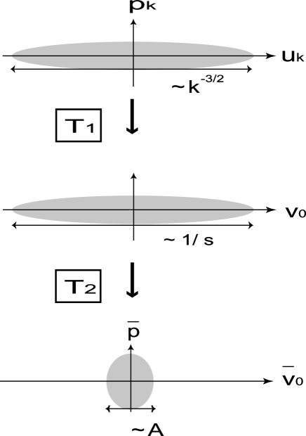
Figure 1: Two Bogoliubov transformations

Now we move on to the second step of transformation. Here we introduce another mode function for $p=0$ mode which naturally defines wave packets with a finite width even in the limit $s_{\bar{\alpha}}\rightarrow 0$ and $V_{c}\rightarrow\infty$. In Fig. 1, we depicted the changes of the wave packets under these two Bogoliubov transformations. For brevity, we have suppressed the indices $I$ and $\alpha$. We denote a new set of mode functions by $\{\bar{v}^{I}_{~{}{\alpha},\hbox{\boldmath{\scriptsize$p$}}}\}$, which is defined by

$$\bar{v}^{I}_{~{}{\alpha},0}(x) \!=\! \cosh r_{{\alpha}}~{}v^{I}_{~{}{\alpha},0}(x)-\sinh r_{{\alpha}}~{}v^{I~{}~{}*}_{~{}{\alpha},0}(x),$$ (121)

$$\bar{v}^{I}_{~{}{\alpha},\hbox{\boldmath{\scriptsize$k$}}}(x) \!=\! v^{I}_{~{}{\alpha},\hbox{\boldmath{\scriptsize$k$}}}(x),$$ (122)

with the squeeze parameter $r_{{\alpha}}$ such that

$$e^{r_{{\alpha}}}=\frac{1}{{\cal N}_{{\alpha}}\!A_{{\alpha}}s_{{\alpha}}}~{},$$ (123)

where $A_{{\alpha}}$ is a real constant. The mode functions for ${\bm{p}}\neq 0$ are unchanged:

$$\bar{v}^{I}_{~{}{\alpha},\hbox{\boldmath{\scriptsize$p$}}}=v^{I}_{~{}{\alpha},\hbox{\boldmath{\scriptsize$p$}}},\quad\mbox{for}~{}{\bm{p}}\neq 0.$$ (124)

We denote the creation and annihilation operators associated with $\{\bar{v}^{I}_{~{}{\alpha},\hbox{\boldmath{\scriptsize$p$}}}\}$ by ${\bar{a}}_{{\alpha}\hbox{\boldmath{\scriptsize$p$}}}^{\dagger}$ and ${\bar{a}}_{{\alpha}\hbox{\boldmath{\scriptsize$p$}}}$.

In the limit $s_{{\alpha}}\rightarrow 0$, we obtain

$$\bar{v}^{I}_{\,{\alpha},0}(x) = V_{c}^{\frac{1}{2}}\Biggl{[}A_{{\alpha}}g^{I}_{\,{\alpha},0}(t)+\frac{i}{A_{{\alpha}}}\frac{1}{V_{c}}\,d^{I}_{\,{\alpha},0}(t)$$

$$\qquad\qquad+\frac{i}{A_{{\alpha}}}\frac{1}{V_{c}}\sum_{\hbox{\boldmath{\scriptsize$p$}}\neq 0}\frac{W_{\hbox{\boldmath{\scriptsize$p$}}}}{W_{0}}d^{I}_{\,{\alpha},p}(t)e^{i\hbox{\boldmath{\scriptsize$p$}}\cdot\hbox{\boldmath{\scriptsize$x$}}}\Biggr{]}~{},$$

The first and the second terms in Eq. (LABEL:v0b) originate from the homogeneous mode, $u^{I}_{~{}{\alpha},0}$, and its complex conjugate. The terms that diverge in the limit $s_{{\alpha}}\to 0$ are common in $u^{I}_{~{}{\alpha},0}$ and $u^{I}_{~{}{\alpha},0}{}^{*}$, which cancel with each other in the definition of $\bar{v}^{I}_{~{}{\alpha},0}$ in Eq. (121). The third term in Eq. (LABEL:v0b) originates from the inhomogeneous modes, $u^{I}_{\,\alpha,p\neq 0}$. The contribution from $u^{I}_{~{}\alpha,p\neq 0}$ is also large in $v^{I}_{\,\alpha,0}$ in the IR limit, but it is not in $\bar{v}^{I}_{\,\alpha,0}$ . The leading terms of $d^{I}_{~{}{\alpha},p}(t)$ in ${\bm{p}}\rightarrow 0$ limit behaves as

$$d^{I}_{~{}{\alpha},p}(t)\approx d^{I}_{~{}{\alpha}}(t)~{}.$$

Hence, the momentum integral $\int d^{3}\bm{p}\,W_{\hbox{\boldmath{\scriptsize$p$}}}d^{I}_{\,{\alpha},p}(t)e^{i{\hbox{\boldmath{\scriptsize$p$}}}\cdot{\hbox{\boldmath{\scriptsize$x$}}}}$, which arises in the continuum limit, remains finite for $x<\infty$.

Here, we choose the unspecified constant $A_{{\alpha}}$ such that the mode functions $\bar{v}^{I}_{{\alpha},0}$ take the minimum amplitude on average. To do so, we compare the amplitude of the first term with that of the last term in Eq. (LABEL:v0b). Near the final time $t_{f}$ the last term is negligibly small, but it is larger in the past. Assuming $\dot{\phi}$ and $H$ are almost constant, the relative amplitude between these two terms is roughly estimated as $|A_{\alpha}^{-2}\int_{0}^{aH}d^{3}p\,d^{I}_{~{}{\alpha},p}|\approx H^{2}/A_{\alpha}^{2}$, where we used $d^{I}_{~{}{\alpha},p}\approx 1/(6Ha^{3})\delta^{I}_{\,{\alpha}}$. Hence, we find that it is appropriate to choose $A_{\bar{\alpha}}=H$ to minimize the amplitude of the mode functions. (We choose $A_{1}=1/s_{1}=\infty$ so that the mode function for the adiabatic mode is unchanged: $\bar{v}^{I}_{1,0}=v^{I}_{1,0}$.)

Now, sending $V_{c}\rightarrow\infty$, we take the continuum limit. We have summarized the correspondence between the discrete description and the continuous one in Appendix A. The overall factor $V_{c}^{\frac{1}{2}}$ in Eq. (LABEL:v0b) is cancelled by $V_{c}^{-\frac{1}{2}}$ in Eq.(55). In this limit, $\sum_{k}$ is replaced with $(2\pi)^{-3}V_{c}\int d^{3}k$. Since the expression (LABEL:v0b) has a factor $1/V_{c}$ in front of the summation $\sum_{k}$, we find that $\bar{v}^{I}_{~{}{\alpha},0}$ is free from the explicit divergence in the limit $V_{c}\to\infty$. In the continuum limit, $\breve{\varphi}^{I}_{1}$ can be expanded as

$$\breve{\varphi}^{I}_{1}(x)\! =\! \sum_{{\alpha}}\left\{{\bar{v}^{I}_{~{}{\alpha},0}\over M_{\rm pl}}{\bar{a}}_{{\alpha},0}+\int_{\hbox{\boldmath{\scriptsize$p$}}\neq 0}\!\frac{d^{3}{\bm{p}}}{(2\pi)^{\frac{3}{2}}}{\bar{v}^{I}_{~{}{\alpha},\hbox{\boldmath{\scriptsize$p$}}}(t)\over M_{\rm pl}}{\bar{a}}_{\alpha,{\hbox{\boldmath{\scriptsize$p$}}}}\right\}$$ (127)

$$\qquad\qquad+(\mbox{h.c.})~{},$$

where

$$\bar{v}^{I}_{\,{\alpha},0}(x)\! =\! H_{f}g^{I}_{\,{\alpha},0}(t)+\frac{i}{H_{f}}\int_{\hbox{\boldmath{\scriptsize$p$}}\neq 0}\frac{d^{3}\bm{p}}{(2\pi)^{3}}\frac{W_{\hbox{\boldmath{\scriptsize$p$}}}}{W_{0}}d^{I}_{\,{\alpha},p}(t)e^{i\hbox{\boldmath{\scriptsize$p$}}\cdot\hbox{\boldmath{\scriptsize$x$}}}~{},$$

$$\bar{v}^{I}_{\,{\alpha},\hbox{\boldmath{\scriptsize$p$}}}(x)\! =\! u^{I}_{\,{\alpha},p}(t)e^{i\hbox{\boldmath{\scriptsize$p$}}\cdot\hbox{\boldmath{\scriptsize$x$}}}-\frac{W_{-\hbox{\boldmath{\scriptsize$p$}}}}{W_{0}}{g^{I}_{\,{\bar{\alpha}},0}(t)\over c_{{\alpha}}(p)}~{}.$$ (129)

B.2 Expansion by coherent states

In this subsection, we show that the adiabatic vacuum state $|\,0\,\rangle_{a}$ can be expanded in terms of the coherent states $|\beta\rangle_{{\bar{a}}}$ associated with ${\bar{a}}_{{\alpha},0}$. The coherent state $|\beta\rangle_{{\bar{a}}}$ is defined by

$$|\beta\rangle_{{\bar{a}}}\equiv\prod_{{\bar{\alpha}}=2}^{D}e^{\beta_{{\bar{\alpha}}}({\bar{a}}_{{\bar{\alpha}},0}^{\dagger}-{\bar{a}}_{{\bar{\alpha}},0})}|\,0\,\rangle_{{\bar{a}}}=\prod_{{\bar{\alpha}}=2}^{D}e^{-\frac{\beta_{{\bar{\alpha}}}^{2}}{2}}e^{\beta_{{\bar{\alpha}}}{\bar{a}}_{{\bar{\alpha}},0}^{\dagger}}\,|\,0\,\rangle_{{\bar{a}}}~{},$$

(130)

where $|\,0\,\rangle_{{\bar{a}}}$ is the vacuum state annihilated by ${\bar{a}}_{{\bar{\alpha}},\hbox{\boldmath{\scriptsize$k$}}}$. This new vacuum state $|\,0\,\rangle_{{\bar{a}}}$ is related to $|\,0\,\rangle_{a}$ by

$$|\,0\,\rangle_{a}=\prod_{{\bar{\alpha}}=2}^{D}(\cosh r_{{\bar{\alpha}}})^{-1/2}e^{\frac{1}{2}\!\tanh r_{{\bar{\alpha}}}\,({\bar{a}}_{{\bar{\alpha}},0}^{\dagger})^{2}}\,|\,0\,\rangle_{{\bar{a}}}~{}.$$ (131)

It is easy to verify that the left hand side is annihilated by $b_{{\bar{\alpha}},0}=(\cosh r_{{\bar{\alpha}}})\,{\bar{a}}_{{\bar{\alpha}},0}-(\sinh r_{{\bar{\alpha}}})\,{\bar{a}}_{{\bar{\alpha}},0}^{\dagger}$. The coherent state satisfies

$${\bar{a}}_{{\bar{\alpha}},\hbox{\boldmath{\scriptsize$p$}}}|\beta\rangle_{{\bar{a}}}=\beta_{{\bar{\alpha}}}|\beta\rangle_{{\bar{a}}}~{},$$

$${\bar{a}}_{1,\hbox{\boldmath{\scriptsize$p$}}}|\beta\rangle_{{\bar{a}}}=0~{}.$$

The original vacuum state $|\,0\,\rangle_{a}$ can be expressed as a superposition of the new coherent states like

$$|\,0\,\rangle_{a} = \prod_{{\bar{\alpha}}=2}^{D}\left[\int^{\infty}_{-\infty}d\beta_{{\bar{\alpha}}}\,E_{{\bar{\alpha}}}(\beta_{{\bar{\alpha}}})\right]\,|\beta\rangle_{{\bar{a}}}~{},$$ (132)

where the coefficient $E_{{\bar{\alpha}}}({\beta_{{\bar{\alpha}}}})$ is given by

$$E_{{\bar{\alpha}}}(\beta_{{\bar{\alpha}}}) \equiv (2\pi\sinh r_{{\bar{\alpha}}})^{-1/2}e^{-\beta_{{\bar{\alpha}}}^{2}(e^{2r_{{\bar{\alpha}}}}-1)^{-1}}$$ (133)

$$\to \sqrt{s_{{\bar{\alpha}}}H_{f}\over\pi}e^{-(s_{{\bar{\alpha}}}H_{f}\beta_{{\bar{\alpha}}})^{2}},~{}(s_{{\bar{\alpha}}}\to 0).~{}$$ (134)

The formula (132) can be verified simply by performing Gaussian integral about $\{\beta_{{\bar{\alpha}}}\}$.

References

- (1) D. Boyanovsky and H. J. de Vega, Phys. Rev. D 70, 063508 (2004) [arXiv:astro-ph/0406287].
- (2) D. Boyanovsky, H. J. de Vega and N. G. Sanchez, Phys. Rev. D 71, 023509 (2005) [arXiv:astro-ph/0409406].
- (3) D. Boyanovsky, H. J. de Vega and N. G. Sanchez, Nucl. Phys. B 747, 25 (2006) [arXiv:astro-ph/0503669].
- (4) D. Boyanovsky, H. J. de Vega and N. G. Sanchez, Phys. Rev. D 72, 103006 (2005) [arXiv:astro-ph/0507596].
- (5) V. K. Onemli and R. P. Woodard, Class. Quant. Grav. 19, 4607 (2002) [arXiv:gr-qc/0204065].
- (6) T. Brunier, V. K. Onemli and R. P. Woodard, Class. Quant. Grav. 22, 59 (2005) [arXiv:gr-qc/0408080].
- (7) T. Prokopec, N. C. Tsamis and R. P. Woodard, arXiv:0707.0847 [gr-qc].
- (8) M. S. Sloth, Nucl. Phys. B 748, 149 (2006) [arXiv:astro-ph/0604488].
- (9) M. S. Sloth, Nucl. Phys. B 775, 78 (2007) [arXiv:hep-th/0612138].
- (10) D. Seery, JCAP 0711, 025 (2007) [arXiv:0707.3377 [astro-ph]].
- (11) D. Seery, JCAP 0802, 006 (2008) [arXiv:0707.3378 [astro-ph]].
- (12) Y. Urakawa and K. i. Maeda, Phys. Rev. D 78, 064004 (2008) [arXiv:0801.0126 [hep-th]].
- (13) E. Komatsu et al. [WMAP Collaboration], arXiv:0803.0547 [astro-ph].
- (14) N. Bartolo, S. Matarrese and A. Riotto, Phys. Rev. D 65, 103505 (2002) [arXiv:hep-ph/0112261].
- (15) N. Bartolo, E. Komatsu, S. Matarrese and A. Riotto, Phys. Rept. 402, 103 (2004) [arXiv:astro-ph/0406398].
- (16) J. M. Maldacena, JHEP 0305, 013 (2003) [arXiv:astro-ph/0210603].
- (17) S. A. Kim and A. R. Liddle, Phys. Rev. D 74, 063522 (2006) [arXiv:astro-ph/0608186].
- (18) D. Babich, P. Creminelli and M. Zaldarriaga, JCAP 0408, 009 (2004) [arXiv:astro-ph/0405356].
- (19) D. Seery and J. E. Lidsey, JCAP 0506, 003 (2005) [arXiv:astro-ph/0503692].
- (20) D. Seery and J. E. Lidsey, JCAP 0509, 011 (2005) [arXiv:astro-ph/0506056].
- (21) S. Weinberg, Phys. Rev. D 72, 043514 (2005) [arXiv:hep-th/0506236].
- (22) S. Weinberg, Phys. Rev. D 74, 023508 (2006) [arXiv:hep-th/0605244].
- (23) G. I. Rigopoulos, E. P. S. Shellard and B. J. W. van Tent, Phys. Rev. D 73, 083521 (2006) [arXiv:astro-ph/0504508].
- (24) G. I. Rigopoulos, E. P. S. Shellard and B. J. W. van Tent, Phys. Rev. D 73, 083522 (2006) [arXiv:astro-ph/0506704].
- (25) G. I. Rigopoulos, E. P. S. Shellard and B. J. W. van Tent, Phys. Rev. D 76, 083512 (2007) [arXiv:astro-ph/0511041].
- (26) F. Vernizzi and D. Wands, JCAP 0605, 019 (2006) [arXiv:astro-ph/0603799].
- (27) X. Chen, M. x. Huang, S. Kachru and G. Shiu, JCAP 0701, 002 (2007) [arXiv:hep-th/0605045].
- (28) T. Battefeld and R. Easther, JCAP 0703, 020 (2007) [arXiv:astro-ph/0610296].
- (29) S. Yokoyama, T. Suyama and T. Tanaka, Phys. Rev. D 77, 083511 (2008) [arXiv:0711.2920 [astro-ph]].
- (30) S. Yokoyama, T. Suyama and T. Tanaka, JCAP 0902, 012 (2009) [arXiv:0810.3053 [astro-ph]].
- (31) D. Seery, M. S. Sloth and F. Vernizzi, arXiv:0811.3934 [astro-ph].
- (32) A. Naruko and M. Sasaki, Prog. Theor. Phys. 121, 193 (2009) [arXiv:0807.0180 [astro-ph]].
- (33) S. Weinberg, arXiv:0805.3781 [hep-th].
- (34) S. Weinberg, Phys. Rev. D 78, 123521 (2008) [arXiv:0808.2909 [hep-th]].
- (35) S. Weinberg, arXiv:0810.2831 [hep-ph].
- (36) H. R. S. Cogollo, Y. Rodriguez and C. A. Valenzuela-Toledo, JCAP 0808, 029 (2008) [arXiv:0806.1546 [astro-ph]].
- (37) Y. Rodriguez and C. A. Valenzuela-Toledo, arXiv:0811.4092 [astro-ph].
- (38) D. H. Lyth, JCAP 0712, 016 (2007) [arXiv:0707.0361 [astro-ph]].
- (39) N. Bartolo, S. Matarrese, M. Pietroni, A. Riotto and D. Seery, JCAP 0801, 015 (2008) [arXiv:0711.4263 [astro-ph]].
- (40) A. Riotto and M. S. Sloth, JCAP 0804, 030 (2008) [arXiv:0801.1845 [hep-ph]].
- (41) K. Enqvist, S. Nurmi, D. Podolsky and G. I. Rigopoulos, JCAP 0804, 025 (2008) [arXiv:0802.0395 [astro-ph]].
- (42) Y. Urakawa and T. Tanaka, arXiv:0902.3209 [hep-th].
- (43) D. Polarski and A. A. Starobinsky, Class. Quant. Grav. 13, 377 (1996) [arXiv:gr-qc/9504030].
- (44) C. Kiefer, I. Lohmar, D. Polarski and A. A. Starobinsky, Class. Quant. Grav. 24, 1699 (2007) [arXiv:astro-ph/0610700].
- (45) A. A. Starobinsky, Lect. Notes Phys. 246, 107 (1986).
- (46) A. A. Starobinsky and J. Yokoyama, Phys. Rev. D 50, 6357 (1994) [arXiv:astro-ph/9407016].
- (47) K. i. Nakao, Y. Nambu and M. Sasaki, Prog. Theor. Phys. 80, 1041 (1988).
- (48) Y. Nambu and M. Sasaki, Phys. Lett. B 219, 240 (1989).
- (49) M. Morikawa, Phys. Rev. D 42, 1027 (1990).
- (50) M. Morikawa, Prog. Theor. Phys. 77, 1163 (1987).
- (51) T. Tanaka and M. a. Sakagami, Prog. Theor. Phys. 100, 547 (1998) [arXiv:gr-qc/9705054].
- (52) D. Seery, arXiv:0903.2788 [astro-ph.CO].
- (53) C. Gordon, D. Wands, B. A. Bassett and R. Maartens, Phys. Rev. D 63, 023506 (2001) [arXiv:astro-ph/0009131].
- (54) D. H. Lyth and Y. Rodriguez, Phys. Rev. D 71, 123508 (2005) [arXiv:astro-ph/0502578].
- (55) P. R. Jarnhus and M. S. Sloth, JCAP 0802, 013 (2008) [arXiv:0709.2708 [hep-th]].
- (56) A. Roura and E. Verdaguer, arXiv:0709.1940 [gr-qc].
- (57) Y. Urakawa and K. i. Maeda, Phys. Rev. D 77, 024013 (2008) [arXiv:0710.5342 [hep-th]].
- (58) F. Finelli, G. Marozzi, A. A. Starobinsky, G. P. Vacca and G. Venturi, Phys. Rev. D 79, 044007 (2009) [arXiv:0808.1786 [hep-th]].
- (59) N. C. Tsamis and R. P. Woodard, Annals Phys. 253, 1 (1997) [arXiv:hep-ph/9602316].
- (60) N. C. Tsamis and R. P. Woodard, Nucl. Phys. B 474, 235 (1996) [arXiv:hep-ph/9602315].
- (61) J. Garriga and T. Tanaka, Phys. Rev. D 77, 024021 (2008) [arXiv:0706.0295 [hep-th]].
- (62) N. C. Tsamis and R. P. Woodard, arXiv:0708.2004 [hep-th].