Computation of inflationary cosmological perturbations in chaotic inflationary scenarios using the phase-integral method

Abstract

The phase-integral approximation devised by Fröman and Fröman, is used for computing cosmological perturbations in the quadratic chaotic inflationary model. The phase-integral formulas for the scalar and tensor power spectra are explicitly obtained up to fifth order of the phase-integral approximation. We show that, the phase integral gives a very good approximation for the shape of the power spectra associated with scalar and tensor perturbations as well as the spectral indices. We find that the accuracy of the phase-integral approximation compares favorably with the numerical results and those obtained using the slow-roll and uniform approximation methods.

I Introduction

The study of the spectrum of anisotropies of the cosmic microwave background radiation and inhomogeneities in the large scale structure of the universe provides key elements in the study of the early universe. The results reported by WMAP favor inflation [1, 2, 3] over other cosmological scenarios. The present and future observational data will permit us to validate and discriminate among different inflationary models. According to WMAP5 data the power-law inflation, the hybrid inflation and quartic chaotic inflationary models $\lambda\phi^{4}$ are ruled out, while the quadratic chaotic inflationary model $m^{2}\phi^{2}$ agreed with the observational data [1, 4].

In order to compare with observations, we should be able to obtain very accurate results for the predicted power spectrum of primordial perturbations for a variety of inflationary scenarios. In general, most of the inflationary models are not exactly solvable and approximate or numerical methods are mandatory in the computation of the scalar and power spectra. Traditionally, the method of approximation applied in inflationary cosmology is the slow-roll approximation [5], which produces reliable results in inflationary models with smooth potentials, but cannot be improved on a simple way beyond the leading order. Recently, some authors have applied alternative approximations, such as the WKB method with the Langer modification [6, 7, 8], the Green function method [9], and the improved WKB method [10, 11].

Habib et al [13, 12, 14] have successfully applied the uniform approximation method in the calculation of the scalar and tensor power spectra and the corresponding spectral indices for the quadratic and quartic chaotic inflationary models, showing that the the uniform approximation gives more accurate results than the slow-roll approximation. Casadio et al [15] have applied the method of comparison equation to study cosmological perturbations during inflation. The comparison method is based on the uniform approximation proposed by Dingle [16] and Miller [17] and thoroughly discussed by Berry and Mount [18].

Recently [19, 20], the phase-integral approximation [21, 22, 23] has been applied to the calculation of the power spectra and spectral indices in the power-law inflationary model, showing that the phase-integral method gives results which are comparable or better than those obtained using slow-roll or the uniform approximation. It is purpose of this paper to compute approximate solutions for the scalar and tensor power spectra and their corresponding spectral indices for some chaotic inflationary models with the help of the phase-integral approximation method. We show that for the quadratic chaotic inflationary model the fifth-order phase integral approximation gives more accurate results than those obtained using the WKB or uniform approximation methods. For the quartic chaotic inflationary model we also obtain very accurate results but we do not report them since this model is ruled out by the observational data [1].

The article is structured as follows: In Sec. II we apply the phase-integral approximation to the chaotic quadratic inflationary model, we numerically solve the equation governing the scalar and tensor perturbations and compare the results for the power-spectra obtained using the phase-integral approach with those computed with the slow-roll and uniform-approximation methods. In Sec. III we summarize our results.

II Phase-integral approximation for the power spectrum in the $\phi^{2}$ chaotic inflation

In this section we discuss the application of the phase-integral approximation to the computation of the power spectrum in the chaotic inflationary $\frac{1}{2}m^{2}\phi^{2}$ model. We apply the phase-integral approximation in the study of the evolution of the mode $k$ equations for the scalar and tensor perturbations in order to compute the scalar and tensor power spectra. Using the fifth-order phase integral approximation we compute the scalar and tensor power spectra and their corresponding spectral indices. A detailed description of the method is given in reference [19, 20].

II.1 The model

The chaotic inflationary model was introduced by Linde [24, 25], he proposed that the preinflationary universe was chaotic which means that the fields would take different values in different points of the space following a random pattern and inflation will occur in virtually any universe that begins in a chaotic, high energy state and has a scalar field with unbounded potential energy. The simplest form of the inflaton potential $V(\phi)$ in a chaotic model is given by the quadratic potential

$$V(\phi)=\frac{1}{2}m^{2}\phi^{2},$$ (1)

giving as a result a free scalar field with mass $m$.

II.2 Equations of motion

In an inflationary universe driven by a scalar field, the equations of motion for the inflaton $\phi$ and the Hubble parameter $H$ are given by

$$\ddot{\phi} + 3H\dot{\phi}=-\frac{\partial V(\phi)}{\partial\phi},$$ (2)

$$H^{2} = \frac{1}{3M_{\mathrm{Pl}}^{2}}\left[V(\phi)+\frac{1}{2}\dot{\phi}^{2}\right],$$ (3)

where the dots indicate derivatives with respect to physical time $t$. In the quadratic chaotic inflationary model the Eqs. (2) and (3) are not exactly solvable in closed form; they can be solved numerically or using the slow-roll approximation. In the slow-roll approximation [26] we consider that the scalar field $V(\phi)$ varies very slowly $\frac{1}{2}\dot{\phi}^{2}\ll V(\phi)$. Using this approximation, we obtain that Eq. (2) and Eq.(3) for the quadratic chaotic inflationary model reduce to [27]

$$3H\dot{\phi} \simeq -m^{2}\phi,$$ (4)

$$H \simeq \frac{m\phi}{\sqrt{6}\,M_{\mathrm{Pl}}}.$$ (5)

Using Eq. (4) and Eq. (5) we obtain that, in the slow-roll approximation, the expansion factor $a(t)$ and the inflaton field $\phi(t)$ are

$$\phi_{\mathrm{sr}} \simeq \phi_{i}-\sqrt{\frac{2}{3}}m\,M_{\mathrm{Pl}}t,$$ (6)

$$a_{\mathrm{sr}} \simeq a_{i}\exp\left({\frac{m\phi_{i}}{\sqrt{6}\,M_{\mathrm{Pl}}}t-\frac{m^{2}}{6}t^{2}}\right),$$ (7)

where $\phi_{i}$ is a constant of integration corresponding to the initial value of the inflaton. Eq. (7) shows that the Universe expands exponentially during inflation The slow-roll parameter is [9]

$$\epsilon_{1}=\frac{\dot{H}}{H^{2}}=\frac{2\,M_{\mathrm{Pl}}^{2}}{\phi^{2}}.$$ (8)

The inflationary epoch finishes when $\epsilon_{1}=1$, that is $\phi_{\textnormal{f}}=\sqrt{2}\,M_{\mathrm{Pl}}$, when the scalar field starts to oscillate. The mass $m$ of the inflation can be fixed using the amplitude of the density fluctuations detected by WMAP. In order to fit $m$ to the observational data, we demand that $m\simeq 10^{-6}$ [3].

The equations of motion (2) and (3) are numerically integrated in the physical time $t$. We solve the system of coupled differential equations (2) and (3) with the help of the sixth-order Runge-Kutta method [28], which can be written as

$$\ddot{\phi} + 3\displaystyle{\frac{\dot{a}}{a}}\dot{\phi}+\frac{\partial V(\phi)}{\partial\phi}=0,$$ (9)

$$\displaystyle{\frac{\dot{a}}{a}} - \sqrt{6}\,M_{\mathrm{Pl}}\left[2V(\phi)+\dot{\phi}^{2}\right]^{1/2}=0.$$

We choose the initial value of the inflaton as $\phi_{i}=15.4\,\,M_{\mathrm{Pl}}$. Since the evolution of the inflation $\phi$ is governed by a second a second-order differential equation, we need to fix the initial value for the velocity of the scalar field $\dot{\phi}_{i}$, which can be obtained using the slow-roll approximation (6). The initial value for $a_{i}$ is chosen as $a_{i}=1$, the mass of the inflaton $m^{2}=1.89\times 10^{-12}\,M_{\mathrm{Pl}}^{2}$. The initial condition has been selected in order to guarantee enough inflation. In order to find the number of e-folds, we rewrite the system of differential equations (9) as

$$\ddot{\phi} + 3\dot{N}\dot{\phi}+\frac{\partial V(\phi)}{\partial\phi}=0,$$ (10)

$$\dot{N} = \sqrt{6}\,M_{\mathrm{Pl}}\left[2V(\phi)+\dot{\phi}^{2}\right]^{1/2}.$$

We find that the inflation finishes at $t_{f}=1.30\times 10^{7}\,M_{\mathrm{Pl}}^{-1}=3.51\times 10^{-36}\mathrm{s}$, a result that corresponds to $59.84$ e-folds before the scalar field starts to oscillate. Fig. 1 shows the evolution of the scalar field $\phi$.

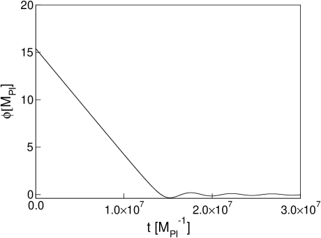
Figure 1: Evolution of the potential $\phi$ for the chaotic inflationary model $\frac{1}{2}m^{2}\phi^{2}$

In order to apply the phase-integral approximation to higher orders it is necessary to calculate the integrals $\omega(z)$ in the complex plane, therefore, it is of help to have an analytic expression for $a(t)$ and $\phi(t)$ which can be obtained after fitting the numerical data. We find that $a(t)$ and $\phi(t)$, take the form

$$a(t) = a_{i}\exp\left(\alpha t-\beta t^{2}\right),$$ (11)

$$\phi(t) = \gamma-\sigma t,$$ (12)

where $\alpha=8.6551\times 10^{-6}\,M_{\mathrm{Pl}}$, $\beta=3.1380\times 10^{-13}\,M_{\mathrm{Pl}}^{2}$, $\gamma=15.3992\,M_{\mathrm{Pl}}$ and $\sigma=1.1201\times 10^{-6}\,M_{\mathrm{Pl}}^{2}$. With the help of the expressions (11) and (12) we obtain that $z_{\mathrm{S}}$ is given by:

$$z_{\mathrm{S}}(t)=-\frac{a_{i}\gamma}{(\alpha-2\beta t)}\exp\left(\alpha t-\beta t^{2}\right).$$ (13)

Fig. 2 and Fig. 2 compare the fitting with the numerical result and the slow-roll approximations for $a(t)$ and $\phi(t)$. The fitting is valid up to $t=5.00\times 10^{6}\,M_{\mathrm{Pl}}^{-1}$. The inset is an enlargement of the figure. Fig. 3 and Fig. 3 show the ratio of the fit and slow-roll to exact solution for $a(t)$ and $\phi(t)$ and observe that the fitting better approximates the numerical result than the slow-roll approximation, therefore the expressions for the scalar and tensor perturbations will be constructed using the fitting $a(t)$ and $z_{\mathrm{S}}(t)$ given by expressions (11) and (13), respectively. If we use $a_{\mathrm{sr}}$ and $\phi_{\mathrm{sr}}$ in order to calculate the power spectrum, the expression we obtain does not approach the exact result.

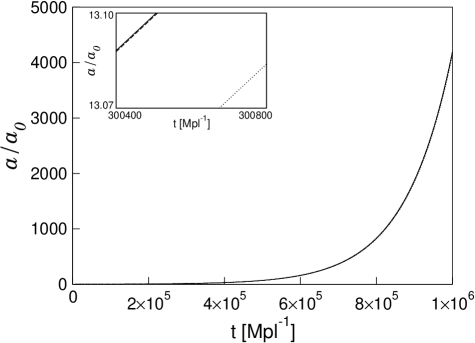
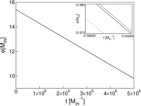
Figure 2: (a) Evolution of the scale factor $a$ and (b) evolution of the inflaton $\phi$ for the chaotic inflationary model $\frac{1}{2}m^{2}\phi^{2}$. Solid line: numerical solution; dashed line: fitting; dotted line: slow-roll approximation. The inset is an enlargement of the figure.

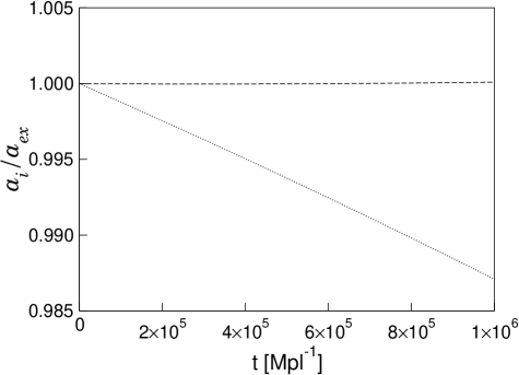
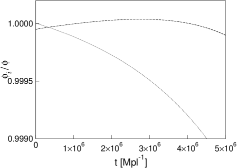
Figure 3: (a) Ratio of the fit and slow-roll to the exact solution for $a(t)$: $a_{i}/a$ and (b) ratio of the fit and slow-roll to the exact solution for $\phi(t)$: $\phi_{i}/\phi$, in the chaotic inflationary model $\frac{1}{2}m^{2}\phi^{2}$. Dashed line: fitting; dotted line: slow-roll approximation.

II.3 Equation for the perturbations

Since the expansion factor $a$ and the field $\phi$ exhibit a simpler form in the physical time $t$ than in the conformal time $\eta$, we proceed to write the equations for the scalar and tensor perturbations in the variable $t$. The relation between $t$ and $\eta$ is given via the equation $dt=a\,d\eta$. In this case, the equation for the perturbations can be written as

$$\ddot{u_{k}}+\frac{\dot{a}}{a}\dot{u_{k}}+\frac{1}{a^{2}}\left[k^{2}-\frac{\left(\dot{a}\dot{z_{\mathrm{S}}}+a\ddot{z_{\mathrm{S}}}\right)a}{z_{\mathrm{S}}}\right]u_{k} = 0,$$ (14)

$$\ddot{v_{k}}+\frac{\dot{a}}{a}\dot{v_{k}}+\frac{1}{a^{2}}\left[k^{2}-\left(\dot{a}^{2}+a\ddot{a}\right)\right]v_{k} = 0.$$ (15)

In order to apply the phase-integral approximation, we eliminate the terms $\dot{u}_{k}$ and $\dot{v}_{k}$ in Eq. (14) and Eq. (15). We make the change of variables $u_{k}(t)=\frac{U_{k}(t)}{\sqrt{a}}$ and $v_{k}(t)=\frac{V_{k}(t)}{\sqrt{a}}$, obtaining that $U_{k}$ and $V_{k}$ satisfy the differential equations:

$$\ddot{U}_{k}+R_{\mathrm{S}}(k,t)U_{k} = 0,$$ (16)

$$\ddot{V}_{k}+R_{\mathrm{T}}(k,t)V_{k} = 0,$$ (17)

with

$$R_{\mathrm{S}}(k,t) = \frac{1}{a^{2}}\left[k^{2}-\frac{\left(\dot{a}\dot{z_{\mathrm{S}}}+a\ddot{z_{\mathrm{S}}}\right)a}{z_{\mathrm{S}}}\right]+\frac{1}{4a^{2}}\left(a^{2}-2a\ddot{a}\right),$$ (18)

$$R_{\mathrm{T}}(k,t) = \frac{1}{a^{2}}\left[k^{2}-\left(\dot{a}^{2}+a\ddot{a}\right)\right]+\frac{1}{4a^{2}}\left(a^{2}-2a\ddot{a}\right),$$ (19)

where $U(k)$ satisfies the asymptotic conditions

$$U_{k} \rightarrow A_{k}\sqrt{a(t)}z_{\mathrm{S}}(t),\quad k\,t\rightarrow\infty$$ (20)

$$U_{k} \rightarrow \sqrt{\frac{a(t)}{2k}}\exp{\left[-ik\eta(t)\right]},\quad k\,t\rightarrow 0,$$ (21)

the asymptotic conditions (20) and (21) also hold for $V_{k}$.

We now proceed to write the explicit equations for quadratic chaotic inflation. From Eq. (18) and Eq. (19), with Eq. (11) and Eq. (12) we obtain

$$R_{\mathrm{S}}(k,t) = \frac{k^{2}}{a_{i}^{2}}\exp\left[-2t(\alpha-\beta t)\right]-\frac{\left[32\beta^{2}+9\left(\alpha-2\beta t\right)^{4}\right]}{4\left(\alpha-2\beta t\right)^{2}}-3\beta,$$ (22)

$$R_{\mathrm{T}}(k,t) = \frac{k^{2}}{a_{i}^{2}}\exp\left[-2t(\alpha-\beta t)\right]-\frac{9}{4}\left(\alpha-2\beta t\right)^{2}+3\beta.$$ (23)

In order to apply the asymptotic condition (21), we use of the relation between $\eta$ and $t$, which is given by:

$$\eta=\frac{\sqrt{\pi}}{2a_{i}\sqrt{\beta}}\exp\left(\frac{-\alpha^{2}}{4\beta}\right)\left[\mathrm{Erfi}\left(\frac{-\alpha+2\beta t}{2\sqrt{\beta}}\right)+\mathrm{Erfi}\left(\frac{\alpha-2\beta t_{0}}{2\sqrt{\beta}}\right)\right],$$ (24)

where $\mathrm{Erfi}(z)$ is the imaginary error function [29]. Since the conformal time $\eta$ is defined up to an integration constant, the lower limit $t_{i}$ of the integral

$$\mathrm{d}\eta=\int_{t_{i}}^{t}\frac{\mathrm{d}t}{a(t)},$$ (25)

is chosen in order to make $\eta=0$ at the end of the inflationary epoch, i.e, $t_{i}=10^{7}\,M_{\mathrm{Pl}}^{-1}$. The dependence of $\eta$ on $t$ is shown in Fig. 4. We can observe that as

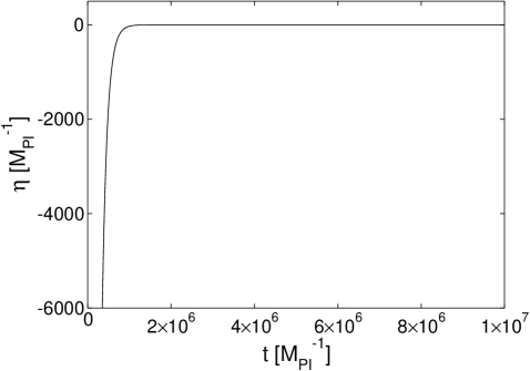
Figure 4: Behavior of $\eta$ as a function of the physical time $t$ for the chaotic inflationary model $\frac{1}{2}m^{2}\phi^{2}$.

$$-k\,\eta\rightarrow 0 \Rightarrow k\,t\rightarrow\infty,$$ (26)

$$-k\,\eta\rightarrow\infty \Rightarrow k\,t\rightarrow 0.$$ (27)

Eq. (16) and Eq. (17), where $R_{\mathrm{S}}(k,t)$ and $R_{\mathrm{T}}(k,t)$ are given by Eq. (22) and Eq. (23), do not possess exact analytic solution. In order to solve the differential equations governing the scalar and tensor perturbations in the physical time $t$, we use the fifth-order phase integral approximation and compare this results with the slow-roll and uniform approximation.

II.4 Phase-integral approximation

In order to solve Eq. (16) and Eq. (17) with the help of the phase-integral approximation, we choose the following base functions $Q$ for the scalar and tensor perturbations

$$Q_{\mathrm{S}}^{2}(k,t) = R_{\mathrm{S}}(k,t),$$ (28)

$$Q_{\mathrm{T}}^{2}(k,t) = R_{\mathrm{T}}(k,t),$$ (29)

where $R_{\mathrm{S}}(k,t)$ and $R_{\mathrm{T}}(k,t)$ are given by Eq. (22) and (23) respectively. Using this selection, the phase-integral approximation is valid as $kt\rightarrow\infty$, limit where we should impose the condition (20), where the validity condition $\mu\ll 1$ holds. The selection, given in Eq. (28), makes the first order phase-integral approximation coincide with the WKB solution. The bases functions $Q_{\mathrm{S}}(k,t)$ and $Q_{\mathrm{T}}(k,t)$ possess turning points $t_{\mathrm{ret}}=\tau_{\mathrm{S}}=1.38096\times 10^{6}\,M_{\mathrm{Pl}}^{-1}$ and $t_{\mathrm{ret}}=\tau_{\mathrm{T}}=t=1.38196\times 10^{6}\,M_{\mathrm{Pl}}^{-1}$, respectively for the mode $k=1.369\,h\,\mathrm{Mpc}^{-1}$. The turning point represents the horizon. There are two ranges where to define the solution. To the left of the turning point $0<t<t_{\mathrm{ret}}$ we have the classically permitted region $Q_{\mathrm{S},\mathrm{T}}^{2}(k,t)>0$ and to the right of the turning point $t>t_{\mathrm{ret}}$ corresponding to the classically forbidden region $Q_{\mathrm{S},\mathrm{T}}^{2}(k,t)<0$, such as it is shown in Figs 5 and Fig. 6.

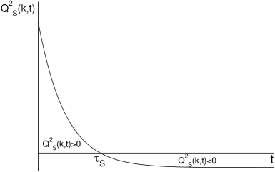
Figure 5: (a) Behavior of the function $Q_{\mathrm{S}}^{2}(k,t)$. (b) Contour of integration $\Gamma_{\tau_{\mathrm{S}}}(t)$ for $0<t<\tau_{\mathrm{S}}$. (c) Contour of integration $\Gamma_{\tau_{\mathrm{S}}}(t)$ for $t>\tau_{\mathrm{S}}$. The dashed line indicates the part of the path on the second Riemann sheet.

Figure 6: (a) Behavior of $Q_{\mathrm{T}}^{2}(k,t)$. (b) Contour of integration $\Gamma_{\tau_{\mathrm{T}}}(t)$ for $0<t<\tau_{\mathrm{T}}$. (c) Contour of integration $\Gamma_{\tau_{\mathrm{T}}}(t)$ for $t>\tau_{\mathrm{T}}$. The dashed lined indicates the part of the path on the second Riemann sheet.

The mode $k$ equations for the scalar an tensor perturbations (16) and (17)in the phase-integral approximation has two solutions: For $0<t<t_{\mathrm{ret}}$

$$u^{\mathrm{pi}}_{k}(t) = \frac{c_{1}}{\sqrt{a(t)}}\left|q_{\mathrm{S}}^{-1/2}(k,t)\right|\cos{\left[\left|\omega_{\mathrm{S}}(k,t)\right|-\frac{\pi}{4}\right]}$$

$$+ \frac{c_{2}}{\sqrt{a(t)}}\left|q_{\mathrm{S}}^{-1/2}(k,t)\right|\cos{\left[\left|\omega_{\mathrm{S}}(k,t)\right|+\frac{\pi}{4}\right]},$$

$$v^{\mathrm{pi}}_{k}(t) = \frac{d_{1}}{\sqrt{a(t)}}\left|q_{\mathrm{T}}^{-1/2}(k,t)\right|\cos{\left[\left|\omega_{\mathrm{T}}(k,t)\right|-\frac{\pi}{4}\right]}$$

$$+ \frac{d_{2}}{\sqrt{a(t)}}\left|q_{\mathrm{T}}^{-1/2}(k,t)\right|\cos{\left[\left|\omega_{\mathrm{T}}(zk,t\right|+\frac{\pi}{4}\right]}.$$

and for $t>t_{\mathrm{ret}}$

$$u^{\mathrm{pi}}_{k}(t) = \frac{c_{1}}{2\sqrt{a(t)}}\left|q_{\mathrm{S}}^{-1/2}(k,t)\right|\exp\left[-\left|\omega_{\mathrm{S}}(k,t)\right|\right]$$

$$+ \frac{c_{2}}{\sqrt{a(t)}}\left|q_{\mathrm{S}}^{-1/2}(k,t)\right|\exp\left[\left|\omega_{\mathrm{S}}(k,t)\right|\right],$$

$$v^{\mathrm{pi}}_{k}(z) = \frac{d_{1}}{2\sqrt{a(t)}}\left|q_{\mathrm{T}}^{-1/2}(k,t)\right|\exp\left[-\left|\omega_{\mathrm{T}}(k,t)\right|\right]$$

$$+ \frac{d_{2}}{\sqrt{a(t)}}\left|q_{\mathrm{T}}^{-1/2}(k,t)\right|\exp\left[\left|\omega_{\mathrm{T}}(k,t)\right|\right].$$

Using the phase-integral approximation up to fifth order ($2N+1=5\rightarrow N=2$), we have that $q_{\mathrm{S}}(k,t)$ and $q_{\mathrm{T}}(k,t)$ can be expanded in the form

$$q_{\mathrm{S}}(k,t)=\sum_{n=0}^{2}Y_{2n_{\mathrm{S}}}(k,t)Q_{\mathrm{S}}(k,t)=\left[Y_{0_{\mathrm{S}}}(k,t)+Y_{2_{\mathrm{S}}}(k,t)+Y_{4_{\mathrm{S}}}(k,t)\right]Q_{\mathrm{S}}(k,t),$$ (34)

$$q_{\mathrm{T}}(k,t)=\sum_{n=0}^{2}Y_{2n_{\mathrm{T}}}(k,t)Q_{\mathrm{T}}(k,t)=\left[Y_{0_{\mathrm{T}}}(k,t)+Y_{2_{\mathrm{T}}}(k,t)+Y_{4_{\mathrm{T}}}(k,t)\right]Q_{\mathrm{T}}(k,t).$$ (35)

In order to compute $q_{\mathrm{S}}(k,t)$ and $q_{\mathrm{T}}(k,t)$, we compute $Y_{2_{\mathrm{S}}}(k,t)$, $Y_{4_{\mathrm{S}}}(k,t)$, $Y_{2_{\mathrm{T}}}(k,t)$, $Y_{4_{\mathrm{T}}}(k,t)$ and the required functions $\varepsilon_{0_{\mathrm{S}}}(k,t)$, $\varepsilon_{2_{\mathrm{S}}}(k,t)$, $\varepsilon_{0_{\mathrm{T}}}(k,t)$ and $\varepsilon_{2_{\mathrm{T}}}(k,t)$. The expressions (34) and (35) give a fifth-order approximation for $q_{\mathrm{S}}(k,t)$ and $q_{\mathrm{T}}(k,t)$. In order to compute $\omega_{\mathrm{S}}(k,t)$ and $\omega_{\mathrm{T}}(k,t)$ we make a contour integration following the path indicated in Figs. 5-(c) 6-(c)

$$\omega_{\mathrm{S}}(k,t) = \omega_{0_{\mathrm{S}}}(k,t)+\sum_{n=1}^{2}\omega_{2n_{\mathrm{S}}}(k,t),$$ (36)

$$= \int_{\tau_{\mathrm{S}}}^{t}Q_{\mathrm{S}}(k,t)\mathrm{d}t+\frac{1}{2}\sum_{n=1}^{2}\int_{\Gamma_{\tau_{\mathrm{S}}}}Y_{2n_{\mathrm{S}}}(k,t)Q_{\mathrm{S}}(k,t)\mathrm{d}t,$$ (37)

$$= \int_{\tau_{\mathrm{S}}}^{t}Q_{\mathrm{S}}(k,t)\mathrm{d}t+\frac{1}{2}\sum_{n=1}^{2}\int_{\Gamma_{\tau_{\mathrm{S}}}}f_{2n_{\mathrm{S}}}(k,t)\mathrm{d}t,$$ (38)

$$\omega_{\mathrm{T}}(k,t) = \omega_{0_{\mathrm{T}}}(k,t)+\sum_{n=1}^{2}\omega_{2n_{\mathrm{T}}}(k,t),$$ (39)

$$= \int_{\tau_{\mathrm{T}}}^{t}Q_{\mathrm{T}}(k,t)\mathrm{d}t+\frac{1}{2}\sum_{n=1}^{2}\int_{\Gamma_{\tau_{\mathrm{T}}}}Y_{2n_{\mathrm{T}}}(k,t)Q_{\mathrm{T}}(k,t)\mathrm{d}t,$$ (40)

$$= \int_{\tau_{\mathrm{S}}}^{t}Q_{\mathrm{T}}(k,t)\mathrm{d}z+\frac{1}{2}\sum_{n=1}^{2}\int_{\Gamma_{\tau_{\mathrm{T}}}}f_{2n_{\mathrm{T}}}(k,t)\mathrm{d}t,$$ (41)

where

$$f_{2n_{\mathrm{S}}}(k,t) = Y_{2n_{\mathrm{S}}}(k,t)Q_{\mathrm{S}}(k,t),$$ (42)

$$f_{2n_{\mathrm{T}}}(k,t) = Y_{2n_{\mathrm{T}}}(k,t)Q_{\mathrm{T}}(k,t).$$ (43)

The functions $f_{2n_{\mathrm{S}}}(k,t)$ and $f_{2n_{\mathrm{T}}}(k,t)$ have the following functional dependence:

$$f_{2_{\mathrm{S}}}(k,t) = A(k,t)(t-\tau_{\mathrm{S}})^{-5/2},$$ (44)

$$f_{4_{\mathrm{S}}}(k,t) = B(k,t)(t-\tau_{\mathrm{S}})^{-11/2},$$ (45)

$$f_{2_{\mathrm{T}}}(k,t) = C(k,t)(t-\tau_{\mathrm{T}})^{-5/2},$$ (46)

$$f_{4_{\mathrm{T}}}(k,t) = D(k,t)(t-\tau_{\mathrm{T}})^{-11/2},$$ (47)

where the functions $A(k,t)$ and $B(k,t)$ are regular at $\tau_{\mathrm{S}}$ and the functions $C(k,t)$, $D(k,t)$ are regular at $\tau_{\mathrm{T}}$. With the help of the functions (44)-(47) we compute the integrals for $\omega_{2n}$ up to $N=4$ using the contour indicated in Figs. 5-(c) and 6-(c). The expressions for $\omega_{2n}$ permit one to obtain the fifth-order phase integral approximation of the solution to the equations for scalar (16) and tensor (17) perturbations. The constants $c_{1}$, $c_{2}$, $d_{1}$ and $d_{2}$ are obtained using the limit $k\,t\rightarrow 0$ of the solutions on the left side of the turning point (II.4) and (II.4), and are given by the expressions

$$c_{1} = -\mathrm{i}\,c_{2},$$ (48)

$$c_{2} = \frac{\mathrm{e}^{-\mathrm{i}\frac{\pi}{4}}}{\sqrt{2}}\mathrm{e}^{-\mathrm{i}\left[k\,\eta(0)+\left|\omega_{0_{\mathrm{S}}}(k,0)\right|\right]},$$ (49)

$$d_{1} = -\mathrm{i}\,d_{2},$$ (50)

$$d_{2} = \frac{\mathrm{e}^{-\mathrm{i}\frac{\pi}{4}}}{\sqrt{2}}\mathrm{e}^{-\mathrm{i}\left[k\,\eta(0)+\left|\omega_{0_{\mathrm{T}}}(k,0)\right|\right]},$$ (51)

In order to compute the scalar and tensor power spectra, we need to calculate the limit as $k\,t\rightarrow\infty$ of the growing part of the solutions on the right side of the turning point given by Eq. (II.4) and Eq. (II.4) for scalar and tensor perturbations respectively.

$$P_{\mathrm{S}}(k) = \lim_{-kt\rightarrow\infty}\frac{k^{3}}{2\pi^{2}}\left|\frac{u_{k}^{\mathrm{pi}}(t)}{z_{\mathrm{S}}(t)}\right|^{2},$$ (52)

$$P_{\mathrm{T}}(k) = \lim_{-kt\rightarrow\infty}\frac{k^{3}}{2\pi^{2}}\left|\frac{v_{k}^{\mathrm{pi}}(t)}{a(t)}\right|^{2}.$$ (53)

II.5 Uniform approximation

We want to obtain an approximate solution to the differential equations (16) and (17) in the range where $Q_{\mathrm{S}}^{2}(k,t)$ and $Q_{\mathrm{T}}^{2}(k,t)$ have a simple root at $t_{\mathrm{ret}}=\tau_{\mathrm{S}}$, and $t_{\mathrm{ret}}=\tau_{\mathrm{T}}$, respectively, so that $Q_{\mathrm{S},\mathrm{T}}^{2}(k,t)>0$ for $0<t<t_{\mathrm{ret}}$ and $Q_{\mathrm{S},\mathrm{T}}^{2}(k,t)<0$ for $t>t_{\mathrm{ret}}$ as depicted in Fig. 5 and Fig. 6. Using the uniform approximation method [18, 13, 19, 20], we obtain that for $0<t<t_{\mathrm{ret}}$ we have

$$U_{k}(k,t) = \left[\frac{\rho_{\mathrm{l}}(k,t)}{Q_{\mathrm{S}}^{2}(k,t)}\right]^{1/4}\left\{C_{1}A_{i}[-\rho_{\mathrm{l}}(k,t)]+C_{2}B_{i}[-\rho_{\mathrm{l}}(k,t)]\right\},$$ (54)

$$V_{k}(k,t) = \left[\frac{\rho_{\mathrm{l}}(k,t)}{Q_{\mathrm{T}}^{2}(k,t)}\right]^{1/4}\left\{C_{1}A_{i}[-\rho_{\mathrm{l}}(k,t)]+C_{2}B_{i}[-\rho_{\mathrm{l}}(k,t)]\right\},$$ (55)

$$\frac{2}{3}\left[\rho_{\mathrm{l}}(k,t)\right]^{3/2} = \int_{t}^{t_{\mathrm{ret}}}\left[Q_{\mathrm{S},\mathrm{T}}^{2}(k,t)\right]^{1/2}\mathrm{d}t,$$ (56)

where $C_{1}$ and $C_{2}$ are two constants to be determined with the help of the boundary conditions (21). For $t>t_{\mathrm{ret}}$

$$U_{k}(k,t) = \left[\frac{-\rho_{\mathrm{r}}(k,t)}{Q_{\mathrm{S}}^{2}(k,t)}\right]^{1/4}\left\{C_{1}A_{i}[\rho_{\mathrm{r}}(k,t)]+C_{2}B_{i}[\rho_{\mathrm{r}}(k,t)]\right\},$$ (57)

$$V_{k}(k,t) = \left[\frac{-\rho_{\mathrm{r}}(k,t)}{Q_{\mathrm{T}}^{2}(k,t)}\right]^{1/4}\left\{C_{1}A_{i}[\rho_{\mathrm{r}}(k,t)]+C_{2}B_{i}[\rho_{\mathrm{r}}(k,t)]\right\},$$ (58)

$$\frac{2}{3}\left[\rho_{\mathrm{r}}(k,t)\right]^{3/2} = \int_{t_{\mathrm{ret}}}^{t}\left[-Q_{\mathrm{S},\mathrm{T}}^{2}(k,t)\right]^{1/2}\mathrm{d}t,$$ (59)

For the computation of the power spectrum we need to take the limit $k\,t\rightarrow\infty$ of the solutions (57) and (58). In this limit we have

$$u_{k}^{\mathrm{ua}}(t) \rightarrow \frac{C}{\sqrt{2\,a(t)}}\left[-Q_{\mathrm{S}}^{2}(k,t)\right]^{-1/2}\left\{\frac{1}{2}\exp\left(-\int_{\tau_{\mathrm{S}}}^{t}\left[-Q_{\mathrm{S}}^{2}(k,t)\right]^{1/2}\mathrm{d}t\right)\right.$$

$$+ \left.\mathrm{i}\,\exp\left(\int_{\tau_{\mathrm{S}}}^{t}\left[-Q_{\mathrm{S}}^{2}(k,t)\right]^{1/2}\mathrm{d}t\right)\right\}$$

$$v_{k}^{\mathrm{ua}}(t) \rightarrow \frac{C}{\sqrt{2\,a(t)}}\left[-Q_{\mathrm{T}}^{2}(k,t)\right]^{-1/2}\left\{\frac{1}{2}\exp\left(-\int_{\tau_{\mathrm{T}}}^{t}\left[-Q_{\mathrm{T}}^{2}(k,t)\right]^{1/2}\mathrm{d}t\right)\right.$$

$$+ \left.\mathrm{i}\,\exp\left(\int_{\tau_{\mathrm{T}}}^{t}\left[-Q_{\mathrm{T}}^{2}(k,t)\right]^{1/2}\mathrm{d}t\right)\right\},$$

where $C$ is a phase factor. Notice that Eq. (II.5) and Eq. (II.5) are identical to Eq. (II.4) and Eq. (II.4) obtained in the first-order phase-integral approximation. Using Eqs. (11), (13) and the growing part of the solutions (II.5) and (II.5) one can compute the scalar and tensor power spectrum using the uniform approximation method,

$$P_{\mathrm{S}}(k) = \lim_{-kt\rightarrow\infty}\frac{k^{3}}{2\pi^{2}}\left|\frac{u_{k}^{\mathrm{ua}}(t)}{z_{\mathrm{S}}(t)}\right|^{2},$$ (62)

$$P_{\mathrm{T}}(k) = \lim_{-kt\rightarrow\infty}\frac{k^{3}}{2\pi^{2}}\left|\frac{v_{k}^{\mathrm{ua}}(t)}{a(t)}\right|^{2}.$$ (63)

We also use the second-order improved uniform approximation for the power spectrum [14],

$$\tilde{P}_{\mathrm{S},\mathrm{T}}(k)=P_{\mathrm{S},\mathrm{T}}(k)\left[\Gamma^{*}(\bar{\nu}_{\mathrm{S},\mathrm{T}})\right],$$ (64)

where $\bar{\nu}_{\mathrm{S},\mathrm{T}}$ is the turning point for the scalar or tensor power spectrum and

$$\Gamma^{*}(\nu)\equiv 1+\frac{1}{12\nu}+\frac{1}{288\nu}-\frac{139}{51840\nu}+\cdots.$$ (65)

II.6 Slow-roll approximation

The scalar and tensor power spectra in the slow-roll approximation to second-order are given by the expressions [9, 30]

$$P_{\mathrm{S}}^{\mathrm{sr}}(k) \simeq \left[1+(4c-2)\epsilon_{1}+2c\delta_{1}+\left(3c^{2}+2c-22+\frac{29\pi^{2}}{12}\right)\epsilon_{1}\delta_{1}+\left(3c^{2}-4+\frac{5\pi^{2}}{12}\right)\delta_{1}^{2}+\right.$$

$$+ \left.\left(-c^{2}+\frac{\pi^{2}}{12}\right)\delta_{2}\right]\left.\left(\frac{H}{2\pi}\right)^{2}\left(\frac{H}{\dot{\phi}}\right)^{2}\right|_{k=aH},$$

$$P_{\mathrm{T}}^{\mathrm{sr}}(k) \simeq \left[1+(2c-2)\epsilon_{1}+\left(2c^{2}-2c-3+\frac{\pi^{2}}{2}\right)\epsilon_{1}^{2}+\left(-c^{2}+2c-2+\frac{\pi^{2}}{12}\right)\epsilon_{2}\right]\left.\left(\frac{H}{2\pi}\right)^{2}\right|_{k=aH},$$ (67)

where $b$ is the Euler constant, $2-\ln 2-b\simeq 0.7296$ and $\ln 2+b-1\simeq 0.2704$, and

$$\epsilon_{1} = \frac{\dot{H}}{H^{2}}=\frac{1}{1+2N_{*}},$$ (68)

$$\epsilon_{2} = \frac{1}{H}\frac{\mathrm{d}\epsilon_{1}}{\mathrm{d}t}=\frac{2}{(1+2N_{*})^{2}},$$ (69)

$$\delta_{n} \equiv \frac{1}{H^{n}\dot{\phi}}\frac{\mathrm{d}^{n+1}\phi}{\mathrm{d}t^{n+1}}\rightarrow\delta_{1}=\delta_{2}=0.$$ (70)

The spectral index in the slow-roll approximation are

$$n_{\mathrm{S}}^{\mathrm{sr}}(k) \simeq 1-4\epsilon_{1}-2\delta_{1}+(8c-8)\epsilon_{1}^{2}+(10c-6)\epsilon_{1}\delta_{1},$$ (71)

$$n_{\mathrm{T}}^{\mathrm{sr}}(k) \simeq -2\epsilon_{1}-2\epsilon_{1}^{2}+(2\alpha-2)\epsilon_{2}.$$ (72)

The expressions (II.6), (67), (71) y (72) depend explicitly on time. In order to compute the scalar and tensor power spectra we need to obtain the dependence on the variable $k$. For a given value of $k$ ($0.0001\,\mathrm{Mpc}^{-1}\leq k\leq 15\,\mathrm{Mpc}^{-1}$) we obtain $t_{*}$ from the relation $k=aH$. Thus, for each $k$ one obtains a value of $t$ that we substitute into $N_{*}$ and Eqs. (II.6), (67), (71) y (72).

II.7 Numerical solution

We integrate on the physical time $t$ the equations (16) and (17) governing the scalar and tensor perturbations using the predictor-corrector Adams method of order $12$ [28], and solve two differential equations, one for the real part and another for the imaginary part $U_{k}$ and $V_{k}$. Two initial conditions are needed in each case $U_{k}(t_{i})$, $U^{\prime}_{k}(t_{i})$, $V_{k}(t_{i})$, $V^{\prime}_{k}(t_{i})$, which can be obtained from the third-order phase-integral approximation. We start the numerical integration at $t_{i}$ calculated at $25$ oscillations before reaching the turning point $t_{\mathrm{ret}}$ [31]. We call this procedure ICs phi3. Figs. 7-9 compare the numerical solution with the fifth-order phase-integral approximation for $\mathrm{Re}(u_{k})$, $\mathrm{Im}(u_{k})$, $\left|u_{k}\right|$, $\mathrm{Re}(v_{k})$, $\mathrm{Im}(v_{k})$, and $\left|v_{k}\right|$. Figures are plotted against the number of e-folds $N$. The solid line corresponds to the numerical solution (ICs phi3), the dashed line corresponds to the fifth-order phase-integral approximation. In each case the turning point $\tau_{\mathrm{S}}$ and $\tau_{\mathrm{T}}$ are indicated with an arrow. We stop the numerical computation of $P_{\mathrm{S}}(k)$ and $P_{\mathrm{T}}(k)$ at $t=5.00\times 10^{6}\,M_{\mathrm{Pl}}^{-1}$, after the mode leaves the horizon, where $u_{k}/z_{\mathrm{S}}$ and $v_{k}/a$ are approximately constant. Notice that the expressions for fitting (11) and (12) are valid in the aforementioned time scales, therefore we can use them for computing the scalar $P_{\mathrm{S}}(k)$ and tensor $P_{\mathrm{T}}(k)$ power spectra.

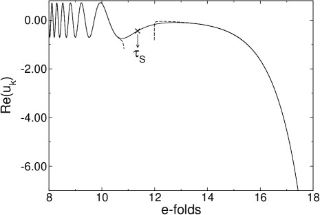
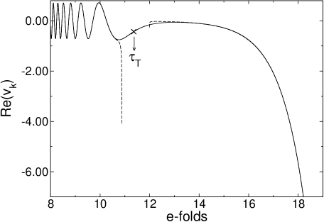
Figure 7: (a) $\mathrm{Re}(u_{k})$ and (b) $\mathrm{Re}(v_{k})$ versus the number of e-folds for the chaotic inflationary model $\frac{1}{2}m^{2}\phi^{2}$. Solid line: numerical solution (ICs phi3); dashed line : fifth-order phase-integral approximation

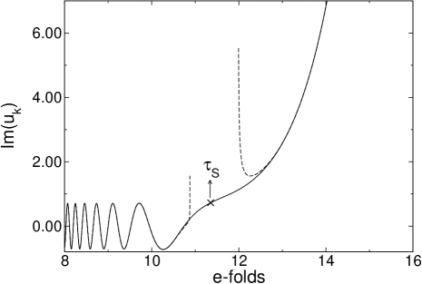
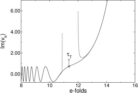
Figure 8: (a) $\mathrm{Im}(u_{k})$ and (b) $\mathrm{Im}(v_{k})$ versus the number of e-folds for the chaotic inflationary model $\frac{1}{2}m^{2}\phi^{2}$. Solid line : numerical result (ICs phi3); dashed line: fifth-order phase-integral approximation

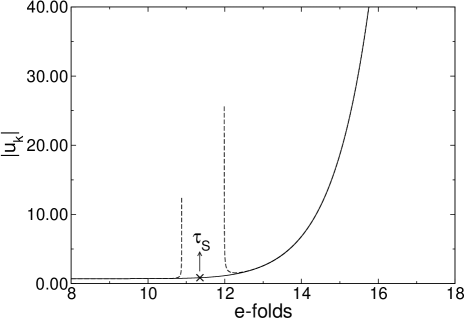
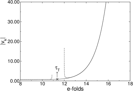
Figure 9: (a) $\left|u_{k}\right|$ and (b) $\left|v_{k}\right|$ versus the number of de e-folds for the chaotic inflationary model $\frac{1}{2}m^{2}\phi^{2}$. Solid line: Numerical result (ICs phi3); dashed line: fifth-order phase-integral approximation

II.8 Results

For the chaotic $\frac{1}{2}m^{2}\phi^{2}$ inflationary model, we want to compare the scalar and tensor power spectra and the spectral indices for different values of $k$ calculated using the third and fifth-order phase-integral approximation with the numerical result (ICs phi3), the first and second-order slow-roll approximation and the first and second-order uniform approximation method. First we analyze the results for the scalar $P_{\mathrm{S}}(k)$ and tensor $P_{\mathrm{T}}(k)$ power spectra shown in Fig. 10 and Fig. 12.

Table 1 shows the value of $P_{\mathrm{S}}(k)$, $P_{\mathrm{T}}(k)$, $n_{\mathrm{S}}(k)$, and $n_{\mathrm{T}}(k)$ using each method of approximation at the WMAP pivot scale. It can be observed that the best value is obtained with the fifth-order phase-integral approximation. It should be noticed that the slow-roll approximation works well since the parameters $\epsilon_{1}$, $\epsilon_{2}$ and $\delta_{n}$ are small.

	num${}^{\text{\tiny{a}}}$	phi3${}^{\text{\tiny{b}}}$	phi5${}^{\text{\tiny{c}}}$	sr1${}^{\text{\tiny{d}}}$	sr2${}^{\text{\tiny{e}}}$	phi1${}^{\text{\tiny{f}}}$, WKB${}^{\text{\tiny{g}}}$, ua1${}^{\text{\tiny{h}}}$	ua2${}^{\text{\tiny{i}}}$
$P_{\mathrm{S}}(k)\times 10^{-11}$	$8.3300$	$8.3419$	$8.3287$	$8.2282$	$8.2299$	$7.4946$	$8.2752$
$P_{\mathrm{T}}(k)\times 10^{-12}$	$1.6109$	$1.6132$	$1.6106$	$1.6047$	$1.6049$	$1.4486$	$1.6004$
$n_{\mathrm{S}}(k)$	$0.960473$	$0.960472$	$0.96473$	$0.960700$	$0.960491$	$0.960453$	$0.960486$
$n_{\mathrm{T}}(k)$	$-0.019965$	$-0.019982$	$-0.019965$	$-0.019650$	$-0.019948$	$-0.020000$	$-0.019984$

Table 1: Value of $P_{\mathrm{S}}(k)$, $P_{\mathrm{T}}(k)$, $n_{\mathrm{S}}(k)$, and $n_{\mathrm{T}}(k)$ obtained with different approximation methods for the chaotic inflationary model $\frac{1}{2}m^{2}\phi^{2}$ for the mode $k=0.05\,\mathrm{Mpc}^{-1}$.

${}^{\text{\tiny{a}}}$Numerical

${}^{\text{\tiny{b}}}$Third-order phase-integral approximation

${}^{\text{\tiny{c}}}$Fifth-order phase-integral approximation

${}^{\text{\tiny{d}}}$First-order slow-roll approximation

${}^{\text{\tiny{e}}}$Second-order slow-roll approximation

${}^{\text{\tiny{f}}}$First-order phase integral approximation

${}^{\text{\tiny{g}}}$WKB approximation

${}^{\text{\tiny{h}}}$First-order uniform approximation

${}^{\text{\tiny{i}}}$Second-order improved uniform approximation

Figures 11 and 13 show the relative error with respect to the numerical result that is obtained using the expression

$$\text{error rel.}\,\,P_{\mathrm{S},\mathrm{T}}(k)=\frac{\left[P_{\mathrm{S},\mathrm{T}}^{\text{\text{approx}}}(k)-P_{\mathrm{S},\mathrm{T}}^{\mathrm{num}}(k)\right]}{P_{\mathrm{S},\mathrm{T}}^{\mathrm{num}}(k)}\times 100.$$ (73)

The first-order phase integral approximation, the WKB and the first-order uniform approximation give the same result, and deviate from the numerical result in $10\%$. The second-order improved uniform approximation gives an error of $0.6\%$. With the first and second-order slow-roll approximation we have an error of $1\%$ for $P_{\mathrm{S}}(k)$ and of $0.4\%$ for $P_{\mathrm{T}}(k)$. Using the third-order phase-integral approximation the error gives $0.15\%$, whereas the fifth-order phase-integral reduces to $0.015\%$ in both cases. Fig. 14 and Fig. 15 show the results for the spectral indices $n_{\mathrm{S}}(k)$ and $n_{\mathrm{T}}(k)$ respectively.

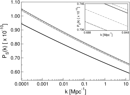
Figure 10: $P_{\mathrm{S}}(k)$ for the chaotic inflationary $\frac{1}{2}m^{2}\phi^{2}$ model. Thin solid line: numerical result (ICs phi3); dot-dashed line: third-order phase-integral approximation, dashed line: fifth-order phase-integral approximation; thick solid line: first-order phase-integral approximation, WKB and first-order uniform approximation, dashed double-dots line: second-order improved uniform approximation, double-dashed dot line: second-order slow-roll approximation, dotted line: first-order slow-roll approximation. The inset is an enlargement of the figure.

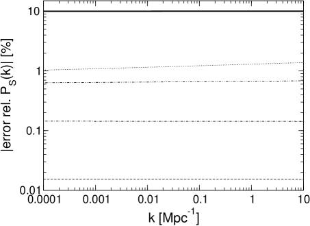
Figure 11: Relative error for $P_{\mathrm{S}}(k)$ for the chaotic inflationary $\frac{1}{2}m^{2}\phi^{2}$ model. Dot-dashed line: third-order phase-integral approximation; dashed line: fifth-order phase-integral approximation; thick solid line: first-order phase-integral approximation; WKB and first-order uniform approximation; dashed double-dots line: second-order improved uniform approximation; dotted line: first and second-order slow-roll approximation. The inset is an enlargement of the figure.

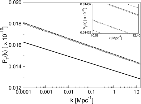
Figure 12: $P_{\mathrm{T}}(k)$ for the chaotic inflationary $\frac{1}{2}m^{2}\phi^{2}$ model. Thin solid line: numerical result (ICs phi3); dot-dashed line: third-order phase-integral approximation; dashed line: fifth-order phase-integral approximation; thick solid line: first-order phase-integral approximation, WKB and first-order uniform approximation; dashed double-dots line: second-order improved uniform approximation; double-dashed dot line: second-order slow-roll approximation; dotted line: first-order slow-roll approximation. The inset is an enlargement of the figure.

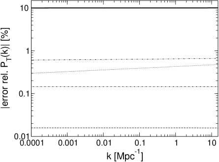
Figure 13: Relative error for $P_{\mathrm{T}}(k)$ for the chaotic inflationary $\frac{1}{2}m^{2}\phi^{2}$ model. Dot-dashed line: third-order phase-integral approximation, dashed line: fifth-order phase-integral approximation; thick solid line: first-order phase-integral approximation; WKB and first-order uniform approximation; dashed double-dots line: second-order improved uniform approximation; dotted line: first and second-order slow-roll approximation. The inset is an enlargement of the figure.

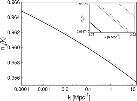
Figure 14: $n_{\mathrm{S}}(k)$ for the chaotic inflationary $\frac{1}{2}m^{2}\phi^{2}$ model. Thin solid line: numerical result (ICs phi3) and fifth-order phase-integral approximation; dot-dashed line: third-order phase-integral approximation;thick solid line: first-order phase-integral approximation; WKB and first-order uniform approximation; dashed double-dots line: second-order improved uniform approximation; double-dashed dot line: second-order slow-roll approximation; dotted line: first-order slow-roll approximation. The inset is an enlargement of the figure.

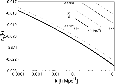
Figure 15: $n_{\mathrm{T}}(k)$ for the chaotic inflationary $\frac{1}{2}m^{2}\phi^{2}$ model. Thin solid line: numerical result (ICs phi3) and fifth-order phase-integral approximation; dot-dashed line: third-order phase-integral approximation; thick solid line: first-order phase-integral approximation; WKB and first-order uniform approximation; dashed double-dots line: second-order improved uniform approximation; double-dashed dot line: second-order slow-roll approximation; dotted line: first-order slow-roll approximation. The inset is an enlargement of the figure.

III Concluding remarks

The results reported in this article show that, in comparison with other approximation methods, the phase integral approach gives very good results for the scalar and tensor spectra in the quadratic inflationary model. The phase-integral approximation gives very accurate results as soon as the the integral $\mu(z,z_{0})$ is small. Figures 7-9 show that the phase integral approximation fails in the vicinity of the turning point $-\nu$, range where the $\mu$-integral diverges. The selection of the base function $Q(z)$ guarantees that $\mu\ll 1$ far from the turning point at any order of approximation. Since the scalar and tensor power spectra as well as the spectral indices are evaluated as $-k\eta\rightarrow 0$, the limit is taken far from the horizon (turning point), therefore their computation is not affected by the presence of the turning point.

Since the WKB method can be regarded as a first-order approximation of the phase-integral approximation with $Q^{2}(z)=R(z)$, it should be expected that the phase-integral method works in those cases where the WKB methods gives good estimates and slow-roll fails, that is the case where inflation is generated by a chaotic potential with a step [32, 15]. The good agreement between the numerical results and those obtained with the phase-integral approximation shows that the phase integral method is a very useful approximation tool for computing the scalar and tensor the power spectra in a wide range of inflationary scenarios.

- [1] E. Komatsu, J. Dunkley, M. R. Nolta, C. L. Bennet, B. Gold, G. Hinshaw, N. Jarosik, D. Larson, M. Limon, L. Page, D. N. Spergel, M. Halpern, R. S. Hill, A. Kogut, S. S. Meyer, G. S. Tucker, J. L. Weiland, E. Wollack, and E. L. Wright, Ap. J. 180, 330 (2009).
- [2] D. N. Spergel, R. Bean, O. Doré, M. R. Nolta, V. L. Bennett, G. Hinshaw, N. Jarosik, E. Komatsu, L. Page, H. Peiris, L. Verde, V. Barnes, M. Halpern, R. S. Hill, A. Kogut, M. Limon, S. S. Meyer, N. Odegard, G. S. Tucker, J. L. Weiland, E. Wollack, and E. L. Wright, Ap. J. 170, 377 (2007).
- [3] D. N. Spergel, L. Verde, H. V. Peiris, E. Komatsu, M. R. Nolta, C. L. Bennett, M. Halpern, G. Hinshaw, N. Jarosik, A. Kogut, M. Limon, S. S. Meyer, L. Page, G. S. Tucker, J. L. Weiland, E. Wollack, and E. L. Wright, Ap. J 148, 175 (2003).
- [4] W. H. Kinney, E. W. Kolb, A. Melchiorri, and A. Riotto, Phys. Rev. D., 78, 087302 (2008).
- [5] E. D. Stewart and D. H. Lyth, Phys. Lett. B 302, 171 (1993).
- [6] R. Langer, Phys. Rev. 51, 669 (1937).
- [7] J. Martin and D. J. Schwarz, Phys. Rev. D 67 083512, (2003).
- [8] R. Casadio, F. Finelli, M. Luzzi, and G. Venturi, Phys. Rev. D 71, 043517 (2005).
- [9] E. D. Stewart and J. Gong. Phys. Lett. B. 510 1 (2001).
- [10] R. Casadio, F. Finelli, M. Luzzi, and G. Venturi Phys. Rev. D 72 103516 (2005).
- [11] R. Casadio, F. Finelli, M. Luzzi, and G. Venturi, Phys. Lett. B 625 1 (2005).
- [12] S. Habib, A. Heinen, K. Heitmann, G. Jungman, and C. Molina-París, Phys. Rev. D, 70 083507, (2004).
- [13] S. Habib, K. Heitmann, G. Jungman, and C. Molina-París, Phys. Rev. Lett. 89, 281301 (2002).
- [14] S. Habib, A. Heinen, K. Heitmann, and G. Jungman, Phys. Rev. D. 71, 043518 (2005).
- [15] R. Casadio, F. Finelli, A Kamenshchik, M Luzzi, and G Venturi, JCAP 0604 (2006) 011
- [16] R. B. Dingle, Appl. Sci. Res. B 5 345, (1956).
- [17] S. C. Miller and R. H. Good, Phys. Rev. D. 91, 174 (1953).
- [18] M. V. Berry , and K. E. Mount, Rep. Prog. Phys. 35, 315 (1972).
- [19] C. Rojas and V. M. Villalba, Phys. Rev. D. 75 063518 (2007).
- [20] V. M. Villalba and C. Rojas, J. Phys.: Conf. Ser. 66 012034 (2007).
- [21] N. Fröman and P. O. Fröman, JWKB Approximation. Contribution to the Theory (North-Holland, Amsterdam, 1965).
- [22] N. Fröman and P.O. Fröman, Phase-Integral Method. Allowing Nearlying Transition Points, volume 40. (Springer Tracts in Natural Philosophy, New York, 1996).
- [23] N. Fröman and P. O. Fröman. Physical Problems Solved by the Phase-Integral Method (Cambridge University Press, Cambridge 2002).
- [24] A. D. Linde. JETP Lett. 38, 176 (1983).
- [25] A. D. Linde Phys. Lett. B. 129, 177 (1983).
- [26] A. R. Liddle and D. H. Lyth. Cosmological Inflation and Large-Scale Structure. (Cambridge University Press, 2000).
- [27] E. J. Copeland, Inflation in the early universe and today. The early universe and observational cosmology, Lecture Notes in Physics 646, 53 (Springer Verlag, Berlin, 2004).
- [28] C. F. Gerald and P. O. Wheatley Applied Numerical Analysis (Addison Wesley, 1984).
- [29] M. Abramowitz and I. Stegun, Handbook of Mathematical Functions (Dover, New York, 1964).
- [30] J. Gong, Clas. Quantum Grav. 21 5555 (2004).
- [31] C. E. Cunha. Evolution of background and perturbation equations in single field inflation models. http://astro.uchicago.edu/ cunha/inflation/node7.html (2005)
- [32] P. Hunt and S. Sarkar, Phys. Rev. D. 70 103518 (2004).