Bond percolation on a class of clustered random networks

Abstract

Analytical results are derived for the bond percolation threshold and the size of the giant connected component in a class of random networks with non-zero clustering. The network’s degree distribution and clustering spectrum may be prescribed, and theoretical results match well to numerical simulations on both synthetic and real-world networks.

Random network models have been extensively studied with a view to gaining insight into the structure and dynamics of many social, technological, and biological networks Newman (2003a); Dorogovtsev and Mendes (2003); Dorogovtsev et al. (2008). However, most analytical approaches rely on tree-like approximations of the local network structure and thus neglect the presence of short loops (cycles) in the graphs. The local clustering coefficient for a node $A$ is defined as the fraction of pairs of neighbors of node $A$ which are also neighbors of each other Watts and Strogatz (1998), and is typically non-negligible in real-world networks. The degree-dependent clustering or clustering spectrum $c_{k}$ is the average of the local clustering coefficient over the class of all nodes of degree $k$ Serrano and Boguñá (2006a); Vázquez et al. (2002). The question of how network models with non-zero $c_{k}$ (taken, for example, from real-world network data) differ from randomly-wired (configuration-model) networks with the same degree distribution $P_{k}$ is of considerable interest.

The bond percolation problem for a network may be stated as follows: each edge of the network graph is visited once, and damaged (deleted) with probability $1-p$. The quantity $p$ is the bond occupation probability and the non-damaged edges are termed occupied. The size of the giant connected component (GCC) of the graph becomes nonzero at some critical value of $p>0$: this critical value of $p$ is termed the bond percolation threshold $p_{th}$. The bond percolation problem has applications in epidemiology, where $p$ is related to the average transmissibility of a disease and the GCC represents the size of an epidemic outbreak Grassberger (1983); Newman (2002), and in the analysis of technological networks, where the resilience of a network to the random failure of links is quantified by the size of the GCC Serrano and Boguñá (2006b). Analytical solutions for percolation on randomly-wired networks and on correlated networks are well-known Molloy and Reed (1995); Callaway et al. (2000); Newman et al. (2001); Vázquez and Moreno (2003), but these cases have zero clustering in the limit of infinite network size.

In this paper we introduce a class of networks with non-zero clustering, and demonstrate analytical solutions for the GCC size and the bond percolation threshold. Most previous studies of clustering effects on percolation rely on numerical simulations using various algorithms to generate clustered networks, e.g. Klemm and Eguiluz (2002); Volz (2004); Serrano and Boguñá (2005). Analytical solutions were found by Newman Newman (2003b) for a bipartite graph model of highly clustered networks. However, the bipartite graph model (in contrast to the model discussed here) is not amenable to fitting to a prescribed degree distribution $P_{k}$. The bipartite graph model of Guillaume and Latapy Guillaume and Latapy (2006) may be fitted to real-world data but their networks do not permit analytical solution of the percolation problem. Serrano and Boguñá Serrano and Boguñá (2006c, b) also obtain approximate analytical solutions, but only for weak clustering cases with $c_{k}<1/(k-1)$. Trapman Trapman (2007) introduced a model of clustering in structured graphs based on embedding cliques (complete subgraphs) within a random tree structure. We show below that this model, and its generalization Gleeson and Melnik (2008) are in fact special cases of the model presented here. In a recent paper Newman (2009), Newman introduced a triangle-based model of clustered networks which may be seen as complementary to the model presented here: we discuss this model in detail at the end of the paper.

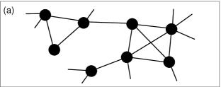
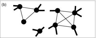
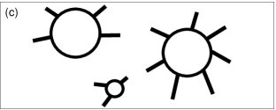
Figure 1: (a) Segment of a clustered random network; (b) split into disjoint cliques, with external links emphasized; (c) corresponding super-nodes.

We consider random networks in which each node may be part of a single clique (a fully-connected subgraph). Figure 1(a) shows a segment of such a network which contains one 3-clique (triangle), one 4-clique, and a single node which is not a member of a clique (for notational convenience we will refer to such individual nodes as members of a 1-clique). Nodes which are members of a $c$-clique have $c-1$ edges linking them to neighbors within the same clique. They also have an additional $k-c+1$ neighbors who are not in the same clique as themselves, where $k$ is the node degree (with $k\geq c-1$). Edges which are not internal to a clique are termed external links. In Fig.1(b) the external links are highlighted with thick lines, but for the purposes of the bond percolation problem they are indistinguishable from clique edges. In networks of this type each node is a member of at most one clique, and so the network can be decomposed into disjoint cliques which are linked together by the set of external links, see Fig. 1(b) . If each clique is regarded as a super-node (Fig. 1(c)) then realizations of the random network may be generated by connecting together randomly chosen pairs of the external link stubs, as in the configuration model for standard random networks Newman et al. (2001).

The fundamental quantity describing networks of this type is the joint probability distribution $\gamma(k,c)$, giving the probability that a randomly-chosen node in the network has degree $k$ and is a member of a $c$-clique. Note $\gamma(k,c)=0$ for $k<c-1$, i.e., $k$-degree nodes can only be members of $c$-cliques if their degree is high enough to provide links to all $c-1$ clique neighbors. The degree distribution $P_{k}$ of the network (probability that a random node has $k$ neighbors) is obtained from $\gamma$ by averaging over all cliques:

$$P_{k}=\sum_{c=1}^{k+1}\gamma(k,c)=\sum_{c}\gamma(k,c).$$ (1)

A node chosen at random from the set of all $k$-degree nodes is a member of a $c$-clique with probability $\gamma(k,c)/P_{k}$. As a member of a $c$-clique, it is part of $\left(\!\!\begin{array}[]{c}c-1\\ 2\end{array}\!\!\right)$ triangles, and so its local clustering coefficient is $\left(\!\!\begin{array}[]{c}c-1\\ 2\end{array}\!\!\right)/\left(\!\begin{array}[]{c}k\\ 2\end{array}\!\right)$. Therefore the degree-dependent clustering coefficient $c_{k}$ is given in terms of $\gamma$ by

$$c_{k}=\sum_{c}\frac{\gamma(k,c)}{P_{k}}\frac{(c-1)(c-2)}{k(k-1)}.$$ (2)

The class of networks described by the joint pdf $\gamma(k,c)$ includes the well-studied configuration model Newman et al. (2001), for which $\gamma(k,c)=\delta_{c1}P_{k}$. This limit contains no cliques, and hence the clustering (in the infinite network size limit) vanishes. Also contained within the class of networks is the Trapman model Trapman (2007); Gleeson and Melnik (2008) in which a fraction $f_{k}$ of $k$-degree nodes form cliques of precisely $k$ nodes, giving $\gamma(k,c)=\delta_{c1}(1-f_{k})P_{k}+\delta_{ck}f_{k}P_{k}$.

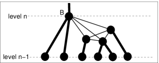
Figure 2: Tree diagram for updating the state of node $B$.

To determine the expected size of the GCC in the damaged network we choose a random node $A$ of the network and approximate the network as a tree structure, with the node $A$ at the top (root) of the tree. Each level of the tree structure (see Fig. 2) is accessed from the level above by traversing one external link. If a node is part of a $c$-clique, the remaining $c-1$ clique neighbors are shown at an intermediate level. Because the graph of super-nodes (Fig. 1(c)) is connected using the configuration model, this tree structure is a locally accurate approximation to the original network is the limit of infinite system size.

To calculate the probability that node $A$ is part of the GCC, we apply a tree-based approach which is generalizable to a variety of cascade dynamics on networks Gleeson (2008) and is related to work on the random field Ising model Dhar et al. (1997). We label nodes which are part of a connected component as active with the remaining nodes termed inactive. All nodes of the tree are initially considered inactive, and we examine the propagation of the active state upwards through the tree (from leaves to root) as an infection process beginning from an infinitesimally small fraction of active nodes infinitely deep in the tree. Consider a node at level $n$, e.g. node $B$ in Fig. 2. Initially $B$ (and its parent at level $n+1$) is inactive, but suppose nodes at level $n-1$ are active with probability $q$. If $B$ has degree $k$, and is a member of a $c$-clique (e.g. $k=6$ and $c=4$ in Fig. 2), it has $k-c+1$ external links, one of which necessarily leads to its parent at level $n+1$. The node $B$ will become active if any one of its $k-c$ externally-linked children at level $n-1$ is active, provided that an occupied edge joins that child to $B$; thus the probability that $B$ is not activated in this fashion is $(1-pq)^{k-c}$. The other mechanism whereby $B$ may be activated is via its neighbors in the $c$-clique; writing $Q_{c}$ for the probability that the top-node (such as $B$) of a $c$-clique is activated by its clique neighbors, we have the total probability of activation for $B$ of $1-(1-pq)^{k-c}(1-Q_{c})$. The probability $Q_{c}$ is calculated using the $P(m|k)$ functions introduced and tabulated in Newman (2003b), which are polynomials in $p$ giving the probability that a randomly chosen node in a damaged (i.e., taking into account bond percolation) $c$-clique belongs to a connected cluster of $m$ nodes (including itself) within the clique. Since node $B$ is activated if any one of its $m-1$ connected neighbors is active, we have

$$Q_{c}=\sum_{m=1}^{c}P(m|c)\left(1-(1-\overline{q}_{c})^{m-1}\right),$$ (3)

where $\overline{q}_{c}$ is the probability of a $c$-clique member at the intermediate level being activated by his level-$(n-1)$ children:

$$\overline{q}_{c}=\sum_{{k^{\prime}}}\frac{\gamma({k^{\prime}},c)}{\sum_{k^{\prime\prime}}\gamma(k^{\prime\prime},c)}\left(1-(1-pq)^{k^{\prime}-c+1}\right).$$ (4)

Here ${\gamma({k^{\prime}},c)}/{\sum_{k^{\prime\prime}}\gamma(k^{\prime\prime},c)}$ is the degree distribution of nodes which are members of cliques of size $c$, and the remaining term is the probability that a ${k^{\prime}}$-degree node in a $c$-clique is activated by one of its ${k^{\prime}}-c+1$ children at level $n-1$.

Given $q$, we can therefore calculate, using equations (3) and (4), the probability of $B$ becoming active. To close the system of equations, we consider the parent of $B$ at level $n+1$, for whom $q$ is the probability that one of its children is active. Since node $B$ has $k-c+1$ external links in total, the probability of it being a child of a random level-$(n+1)$ node is $\Pi_{kc}=(k-c+1)\gamma(k,c)/z_{e}$, where $z_{e}=\sum_{{k^{\prime}},c^{\prime}}({k^{\prime}}-c^{\prime}+1)\gamma({k^{\prime}},c^{\prime})$ is the average number of external links per node. Combining the equations above gives the closure relation

$$q=\sum_{k,c}\Pi_{kc}\left(1-(1-pq)^{k-c}(1-Q_{c})\right)\equiv G(q).$$ (5)

Equations (3)–(5) are solved by iterating from an infinitesimally small value of $q$ to a steady-state solution: this determines the probability (in an infinite network) that a node is active, conditional on its parent being inactive. The final calculation of the GCC size considers the node $A$ at the top (root) of the tree: with probability $\gamma(k,c)$ this has $k-c+1$ direct links to the level below. By similar arguments to before, node $A$ is active with probability

$$S=\sum_{k,c}\gamma(k,c)\left(1-(1-pq)^{k-c+1}(1-Q_{c})\right),$$ (6)

where $q$ is the solution of equations (3)–(5) and $S$ is the expected fractional size of the GCC.

Note that if we set $\gamma(k,c)=\delta_{c1}P_{k}$, equations (5) and (6) reduce to their well-studied configuration model versions (using $Q_{1}=0$). The bond percolation results of Trapman (2007); Gleeson and Melnik (2008) for the generalized Trapman model are also a special case of equations (3)–(6). Also of interest is the GCC size in an undamaged network—this is obtained from our equations by setting $p=1$ (for which $P(m|c)=\delta_{mc}$).

The bond percolation threshold is the value of $p$ at which the GCC size first becomes nonzero. This may be determined from the cascade condition Gleeson and Melnik (2008); Gleeson (2008) $G^{\prime}(0)=1$, where $G(q)$ is defined in equation (5). The resulting polynomial equation for $p$ may be written in the form

$$\frac{1}{z_{e}}\sum_{k,c}(k-c+1)\gamma(k,c)\left(p(k-c)+(z_{c}-c+1)D_{c}(p)\right)=1,$$ (7)

where $D_{c}(p)=p\sum_{m=1}^{c}(m-1)P(m|c)$ (see Gleeson and Melnik (2008)) and $z_{c}$ is the average degree of nodes in cliques of size $c$: $z_{c}=\sum_{k}k\gamma(k,c)/\sum_{{k^{\prime}}}\gamma({k^{\prime}},c)$.

We now describe an algorithm for generating realizations of random networks with a prescribed distribution $\gamma(k,c)$. For a large number $\widetilde{N}$ (which is related to the number $N$ of nodes in the final network, see below), we choose $\widetilde{N}$ random numbers $c_{i}$ ($i=1$ to $\widetilde{N}$) with pdf $\left(\sum_{k}\gamma(k,c)/c\right)/\left(\sum_{k,c^{\prime}}\gamma(k,c^{\prime})/c^{\prime}\right)$ to be the clique sizes in the network realization. For each $c_{i}$, we create $c_{i}$ nodes in a complete subgraph, and assign their degrees $k_{j}$ ($j=1$ to $c_{i}$) by drawing random numbers from a distribution with density $\gamma(k,c_{i})/\sum_{{k^{\prime}}}\gamma({k^{\prime}},c_{i})$. Node $j$ in clique $i$ then has $k_{j}-c_{i}+1$ external link stubs associated with it. Having created all $\widetilde{N}$ cliques in this fashion, we randomly choose pairs of external link stubs and connect them together to create the random network (c.f. Fig. 1). The expected number of nodes in a network generated using this algorithm is $N=\widetilde{N}/\left(\sum_{k,c}\gamma(k,c)/c\right)$, which allows us to estimate the value of $\widetilde{N}$ needed to produce a final network of size $N$. For finite-sized networks, the presence of cliques means this algorithm is not guaranteed to give exactly $N$ nodes in the final network, but in practice we find the variation in the network size is negligibly small for sufficiently large $N$.

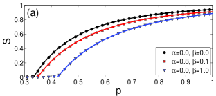
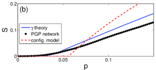
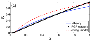
Figure 3: (Color online) Size of giant connected component as a function of bond occupation probability for (a) synthetic networks with Poisson degree distribution; (b) pretty-good-privacy network, for $p$ near $p_{th}$; (c) as (b), but for all $p$ values.

Figure 3(a) shows a comparison between GCC sizes from theory (from equations (3)–(6)) and numerical simulations on networks with the Poisson degree distribution $P_{k}=z^{k}e^{-z}/k!$ and mean degree $z=3$. We create non-zero clustering in the networks by inserting 3-cliques (triangles) and 4-cliques; specifically, we set $\gamma(k,c)=\left((1-\alpha-\beta)\delta_{c1}+\alpha\delta_{c3}+\beta\delta_{c4}\right)P_{k}$ for $k\geq 3$. This embeds a fraction $\alpha$ and $\beta$ of $k$-degree nodes in 3-cliques and 4-cliques, respectively, with the remainder as individuals (i.e, 1-cliques). Since nodes of degree $k$ cannot be part of $c$-cliques when $c$ exceeds $k+1$, we deal with nodes of degree $k<3$ as follows: $\gamma(2,c)=\left((1-\alpha)\delta_{c1}+\alpha\delta_{c3}\right)P_{2}$, and $\gamma(k,c)=P_{k}\delta_{c1}$ for $k=0$ or 1. The case $\alpha=\beta=0$ gives the standard configuration model network, with zero clustering. We also show results for $\alpha=0.8$, $\beta=0.1$ and for $\alpha=0$, $\beta=1$. Using (2), the first of these corresponds to a global clustering coefficient $C=\sum_{k}P_{k}c_{k}$ of 0.31, while the second case, which contains only 4-cliques, has $C=0.35$. The corresponding bond percolation thresholds may be calculated from the polynomial equation (7) using (see Gleeson and Melnik (2008)) $D_{3}(p)=2p^{2}(1+p-p^{2})$ and $D_{4}(p)=3p^{2}(1+2p-7p^{3}+7p^{4}-2p^{5})$. The resulting values are $p_{th}=0.349$ and $p_{th}=0.422$, both exceeding the configuration model value of $p_{th}=1/z=1/3$ Molloy and Reed (1995); Callaway et al. (2000). Numerical simulation results on networks of size $N=10^{5}$ are shown by the symbols, while the curves are the theoretical predictions of equations (3)–(6). The agreement between theory and numerics is excellent.

One of the motivations for the introduction of the $\gamma$ networks is the ability to obtain analytical results for networks with given degree distribution $P_{k}$ and clustering spectrum $c_{k}$. Equations (1) and (2) constrain the distribution $\gamma(k,c)$ to fit a desired $P_{k}$ and $c_{k}$, which may be measured, for example, in a real-world network. However, these constraints still permit significant freedom in choosing $\gamma(k,c)$. It is convenient therefore to consider a parametrization of $\gamma(k,c)$ which allows straightforward fitting to given network data. We suppose that the distribution of clique-sizes $c$ occupied by nodes of degree $k$ is given by a binomial distribution, defining

$$\gamma(k,c)=P_{k}\,\left(\!\!\begin{array}[]{c}k\\ c-1\end{array}\!\!\right)g_{k}^{c-1}(1-g_{k})^{k-c+1},$$ (8)

for $c=1$ to $k+1$. This distribution clearly satisfies (1), and it distributes the probability mass corresponding to the $k$-degree nodes over the $c$-clique sizes via the single parameter $g_{k}$. The relationship between the parameters $g_{k}$ and the clustering spectrum $c_{k}$ is remarkably simple; substituting the parametrization (8) into (2) yields $c_{k}=g_{k}^{2}$. Thus the form (8) for $\gamma$ may immediately be fitted to the $P_{k}$ and $c_{k}$ of a real-world dataset by setting $g_{k}=\sqrt{c_{k}}$.

Figures 3(b) and 3(c) show the results of applying the parametrization (8) to match the degree distribution and clustering spectrum of the connected component of the pretty-good-privacy (PGP) network Boguñá et al. (2004). The PGP network is highly clustered, with $c_{k}>1/(k-1)$ for most $k$ Serrano and Boguñá (2006b). Numerical calculations of the GCC size in this network are shown by the symbols on Fig. 3(b) and 3(c); also shown are the theoretical predictions for the zero-clustering (configuration model) case and the results of equations (3)–(6) with parametrization (8). The effects of clustering on the percolation threshold are well-captured by the $\gamma$ theory, see Fig. 3(b). Note that here, in contrast to the example in Fig. 3(a), clustering acts to decrease the percolation threshold: equation (7) gives $p_{th}=0.0236$, which is less than half the configuration model value of $0.0559$. The $\gamma$ theory gives quite a good approximation to the actual GCC size for bond occupation probabilities of $p$ up to about 0.5 (Fig. 3(c)); however the behavior at larger $p$ values is less accurate, with the predicted GCC in the undamaged ($p=1$) network being substantially smaller than its true value. This inaccuracy may be attributable to excessive clustering being induced by the parametrization (8) for the large $p$ case.

In summary, we have introduced a class of clustered random networks with arbitrary degree distribution and clustering spectrum, and analytically determined the size of the GCC and the bond percolation threshold. Numerically generated networks show excellent agreement with the theoretical results, and we have demonstrated the applicability of the theory by fitting to the pretty-good-privacy network to produce accurate predictions of the GCC size for small $p$. We have used a cascade-based approach here in preference to a generating function method, because (as we show in a subsequent paper) this approach generalizes to give analytical results for $k$-core sizes, Watts’ threshold decision model, and other cascading dynamics on clustered networks Gleeson (2008).

It is instructive to compare our $\gamma$-theory networks with the clustered network model recently introduced by Newman Newman (2009). In his model, a $k$-degree node may be a member of up to $k/2$ disjoint triangles (3-cliques), and thus have a local clustering coefficient of up to $1/(k-1)$. In contrast, nodes in the $\gamma$-theory networks can be members of only a single clique, but using large cliques can give arbitrarily high clustering. The restriction $c_{k}\leq 1/(k-1)$ imposed on Newman’s model networks inhibits a direct fit to most real-world networks, in contrast to our results in Fig. 3. It would be interesting to explore the possibility of modelling networks with multiple cliques per node (as in Newman (2009)) while allowing the cliques to be larger than triangles (as here). Indeed, a general model of this type is proposed in Bollobas et al. (2008) but it seems unlikely that easily computable analytical solutions, as found here and in Newman (2009), can be obtained in this more general setting.

Discussions with Sergey Melnik, Adam Hackett and Mason Porter are gratefully acknowledged. This work was funded by Science Foundation Ireland under programmes 06/IN.1/I366 and MACSI 06/MI/005.

References

- Newman (2003a) M. E. J. Newman, SIAM Rev. 45, 167 (2003a).
- Dorogovtsev and Mendes (2003) S. Dorogovtsev and J. Mendes, Evolution of Networks: From Biological Nets to the Internet and WWW (Oxford University Press, Oxford, 2003).
- Dorogovtsev et al. (2008) S. N. Dorogovtsev, A. V. Goltsev, and J. F. F. Mendes, Rev. Mod. Phys. 80, 1275 (2008).
- Watts and Strogatz (1998) D. J. Watts and S. H. Strogatz, Nature (London) 393, 440 (1998).
- Serrano and Boguñá (2006a) M. Á. Serrano and M. Boguñá, Phys. Rev. E 74, 056114 (2006a).
- Vázquez et al. (2002) A. Vázquez, R. Pastor-Satorras, and A. Vespignani, Phys. Rev. E 65, 066130 (2002).
- Grassberger (1983) P. Grassberger, Math. Biosci. 63, 157 (1983).
- Newman (2002) M. E. J. Newman, Phys. Rev. E 66, 016128 (2002).
- Serrano and Boguñá (2006b) M. Á. Serrano and M. Boguñá, Phys. Rev. E 74, 056115 (2006b).
- Molloy and Reed (1995) M. Molloy and B. Reed, Random Structures and Algorithms 6, 161 (1995).
- Callaway et al. (2000) D. S. Callaway, M. E. J. Newman, S. H. Strogatz, and D. J. Watts, Phys. Rev. Lett. 85, 5468 (2000).
- Newman et al. (2001) M. E. J. Newman, S. H. Strogatz, and D. J. Watts, Phys. Rev. E 64, 026118 (2001).
- Vázquez and Moreno (2003) A. Vázquez and Y. Moreno, Phys. Rev. E 67, 015101(R) (2003).
- Klemm and Eguiluz (2002) K. Klemm and V. M. Eguiluz, Phys. Rev. E 65, 036123 (2002).
- Volz (2004) E. Volz, Phys. Rev. E 70, 056115 (2004).
- Serrano and Boguñá (2005) M. Á. Serrano and M. Boguñá, Phys. Rev. E 72, 036133 (2005).
- Newman (2003b) M. E. J. Newman, Phys. Rev. E 68, 026121 (2003b).
- Guillaume and Latapy (2006) J.-L. Guillaume and M. Latapy, Physica A 371, 795 (2006).
- Serrano and Boguñá (2006c) M. Á. Serrano and M. Boguñá, Phys. Rev. Lett. 97, 088701 (2006c).
- Trapman (2007) P. Trapman, Theor. Pop. Biol. 71, 160 (2007).
- Gleeson and Melnik (2008) J. P. Gleeson and S. Melnik, arXiv (2008), eprint arXiv:0811.4511 (submitted to Phys. Rev. E).
- Newman (2009) M. E. J. Newman, Phys. Rev. Lett. 103, 058701 (2009).
- Gleeson (2008) J. P. Gleeson, Phys. Rev. E 77, 046117 (2008).
- Dhar et al. (1997) D. Dhar, P. Shukla, and J. P. Sethna, J. Phys. A 30, 5259 (1997).
- Boguñá et al. (2004) M. Boguñá, R. Pastor-Satorras, A. Diaz-Guilera, and A. Arenas, Phys. Rev. E 70, 056122 (2004).
- Bollobas et al. (2008) B. Bollobas, S. Janson, and O. Riordan, arXiv (2008), eprint arXiv:0807.2040.