RR Lyrae Variables in Two Fields in the Spheroid of M31

Abstract

We present Hubble Space Telescope observations taken with the Advanced Camera for Surveys Wide Field Channel of two fields near M32 - between four and six kpc from the center of M31. The data cover a time baseline sufficient for the identification and characterization of 681 RR Lyrae variables of which 555 are ab-type and 126 are c-type. The mean magnitude of these stars is $\langle$$V$$\rangle$$=25.29\pm 0.05$ where the uncertainty combines both the random and systematic errors. The location of the stars in the Bailey Diagram and the ratio of c-type RR Lyraes to all types are both closer to RR Lyraes in Oosterhoff type I globular clusters in the Milky Way as compared with Oosterhoff II clusters. The mean periods of the ab-type and c-type RR Lyraes are $\langle$$P_{ab}$$\rangle$$=0.557\pm 0.003$ and $\langle$$P_{c}$$\rangle$$=0.327\pm 0.003$, respectively, where the uncertainties in each case represent the standard error of the mean. When the periods and amplitudes of the ab-type RR Lyraes in our sample are interpreted in terms of metallicity, we find the metallicity distribution function to be indistinguishable from a Gaussian with a peak at $\langle$[Fe/H]$\rangle$=$-1.50\pm 0.02$, where the quoted uncertainty is the standard error of the mean. Using a relation between RR Lyrae luminosity and metallicity along with a reddening of $E(B-V)=0.08\pm 0.03$, we find a distance modulus of $(m-M)_{0}=24.46\pm 0.11$ for M31. We examine the radial metallicity gradient in the environs of M31 using published values for the bulge and halo of M31 as well as the abundances of its dwarf spheroidal companions and globular clusters. In this context, we conclude that the RR Lyraes in our two fields are more likely to be halo objects rather than associated with the bulge or disk of M31, in spite of the fact that they are located at 4-6 kpc in projected distance from the center.

1 Introduction

Pulsating variable stars such as RR Lyraes are powerful probes useful for investigating the properties of stellar populations. The mere presence of RR Lyraes among a population of stars suggests an ancient origin since ages older than $\sim$10 Gyr are required to produce RR Lyrae variables. Their periods and amplitudes are a reflection of the metal abundance of the population. Along with their incredible usefulness, RR Lyraes are also relatively straightforward to identify and characterize. This is because of their short periods and the distinct light curve shapes of the ab-types, which pulsate in the fundamental mode and exhibit a relatively rapid rise to maximum and a gradual decline to minimum. This is in contrast to the c-type RR Lyraes which pulsate in the first harmonic and show light curves that are more akin to sine curves. In spite of the great potential RR Lyraes hold as astrophysical tools, they have not been widely studied in our nearest large neighbor galaxy, Andromeda.

One of the first studies attempting to identify RR Lyraes in M31 was that of Pritchet & van den Bergh (1987). They used the Canada-France-Hawaii 3.6m telescope to observe a field at a distance of 9 kpc from the center of M31 along the minor axis partially overlapping the field observed by Mould & Kristian (1986). They identified 30 RR Lyrae candidates and were able to estimate periods for 28 of them. These ab-type variables have a mean period of $\langle$$P_{ab}$$\rangle$=0.548 days. The photometric errors in their data prevented them from identifying the lower-amplitude c-type RR Lyraes.

The RR Lyrae variables in M31 globular clusters have been investigated by Clementini et al. (2001, cf. Contreras et al. 2008). They used the Wide Field Planetary Camera 2 (WFPC2) onboard the Hubble Space Telescope (HST) to make the first tentative detection of RR Lyraes in G11, G33, G64, and G322, finding two, four, 11, and eight variables, respectively. Detection and characterization of these stars in globular clusters is more challenging than in the M31 field because of the increased crowding.

Returning to the work on field RR Lyraes, Dolphin et al. (2004) observed the same field as Pritchet & van den Bergh (1987) using the WIYN 3.5m on Kitt Peak. They found 24 RR Lyrae stars with a completeness fraction of 24%, suggesting that their $\sim$100 square arcmin field could contain $\sim$100 RR Lyraes resulting in a density of one RR Lyrae per square arcmin. This is much less than the value of $\sim$17 per square arcmin found by Pritchet & van den Bergh (1987). They also noted for the first time that the mean metallicity of the M31 RR Lyraes seemed to be significantly lower than that of the M31 halo. The work of Durrell et al. (2001) had reported a peak value of $[M/H]$$\sim$–0.8 for the M31 halo. Dolphin et al. (2004) were not able to reconcile this abundance value with the distance implied by the mean magnitude of their RR Lyrae sample.

The first definitive work on the RR Lyraes of M31 was published by Brown et al. (2004, hereafter B2004) and made use of $\sim$84 hours of imaging time (250 exposures over 41 days) with the Advanced Camera for Surveys onboard HST. Their field was located along the minor axis of M31 approximately 11 kpc from its center. Their analysis revealed a complete sample of RR Lyrae stars consisting of 29 ab-type variables and 25 c-type. The periods of these stars suggest a mean metallicity of $[Fe/H]$$\sim$-1.6 for the old population in the Andromeda halo. This is qualitatively consistent with the assertions of Dolphin et al. (2004) regarding the metal abundance of the M31 halo - that it is lower than the value suggested by the work of Durrell et al. (2001). More recent work has shown that the M31 halo extends from 30 to 165 kpc (Guhathakurta et al. 2005; Irwin et al. 2005) and has a metallicity that is actually closer to that of the Milky Way halo (Kalirai et al. 2006; Koch et al. 2008).

There is one more paper of note related to this topic and that is the work of Alonso-García et al. (2004). They used the Wide Field Planetary Camera 2 onboard HST to image a field $\sim$3.5 arcmin to the east of M32 and compared it with a control field that samples the M31 field stars well away from M32. They identify variable stars that they claim are RR Lyraes belonging to M32 therefore suggesting that M32 possesses a population that is older than $\sim$10 Gyr. They were not able to classify the RR Lyraes or derive periods and amplitudes for them so their results are not directly comparable to ours.

This review of the literature reveals a significant deficiency in the spatial coverage of RR Lyrae studies in the vicinity of M31. Given the great astrophysical utility of RR Lyrae variables and the expansive size of M31 on the sky, it is clear that a survey of these stars sampling a diversity of regions in Andromeda will provide valuable insights into the star formation and chemical enrichment history of our nearest spiral neighbor.

With this in mind, this paper presents the results of archival HST/ACS observations showcasing the RR Lyrae population in the inner regions of the M31 spheroid. The next section describes the observational material and the photometric procedure. We move on to describe the technique used to identify and characterize the variable stars in Sec. 3. The results of this study are described in Sec. 4, and a discussion of these results within the broader context of the M31 halo are presented in Sec. 5. Our conclusions are then summarized in Sec. 6.

2 Observations

The observations used in the present study were obtained with the Hubble Space Telescope Advanced Camera for Surveys (HST/ACS) in parallel with the imagery conducted by program GO-10572. The primary goal of this program was to obtain a deep color-magnitude diagram of the envelope of M32, using the High Resolution Channel (HRC) of the ACS. The total envelope exposure was 32 orbits, split between two filters. An identical set of HRC exposures was later obtained in a background field selected to represent the M31 disk+halo contribution to the M32 envelope exposures. The present images are the parallel observations associated with each pointing obtained with the ACS Wide Field Channel (WFC) using the F606W ($\sim$V) filter. Table 1 provide some details of the observational data. The temporal coverage is 2.2 days for field 1 and 3.1 days for field 2.

Figure 1 shows the locations of these fields relative to M31. While the M32-background field was carefully selected to fall along the M31 isophote that ran through the M32 envelope field, the two fields were significantly separated in time, thus different spacecraft rolls between the two epochs caused the parallel WFC aperture to fall randomly about the primary HRC fields. Field 1 thus samples a region that is 4.5 kpc in projected distance from the center of M31, while Field 2 is located 6.6 kpc from the center. Note that throughout this paper, we adopt an M31 distance modulus of $(m-M)_{o}=24.43$ corresponding to a distance of 770 kpc (Freedman & Madore 1990).

The spacecraft was dithered in a complex pattern to both achieve Nyquist-sampling in the HRC and rejection of CCD defects. Each pair of orbits was dithered in a $2\times 2$ square pattern of 0.5 HRC pixel steps, followed by larger steps to trace a skewed-square spiral of $\sim 0.2$ arcsec total amplitude over the 16 total orbits devoted to each filter/field combination. The subpixel dithering to achieve Nyquist sampling in the HRC is not optimal for the $2\times$ larger pixels of the WFC, but the larger-scale dither pattern fortunately served to offer diverse sampling information for the parallel imagery.

3 Reductions

3.1 Photometry of Program Frames

We chose to work on the FLT images as retrieved from the HST archive. These frames have been bias-subtracted and flat-fielded, but, unlike the drizzled (DRZ) images, they retain the geometric distortions of ACS (Mahmud & Anderson 2008). Photometry was performed using the same procedure as Sarajedini et al. (2006). The first step is the application of geometric correction images to the Wide Field Channel 1 and 2 (WFC1 and WFC2, respectively) portions of the FLT images. After this step, the data quality maps are applied where the values of the bad pixels in the science images are set to a number well below the sky background to be sure the photometry software ignores those pixels. At this point, the resultant images are ready to be photometered.

The detection of the stellar profiles and the measurement of magnitudes was done with the DAOPHOT/ALLSTAR/ALLFRAME crowded-field photometry software (Stetson 1987; 1994). After the application of the standard FIND and PHOT routines to detect stars and perform aperture photometry on them, ALLSTAR was applied to each of the 32 images in order to derive well-determined positions for all of the stars. In this step and in subsequent ones involving the application of a point-spread function (PSF) in order to determine positions and magnitudes, we made use of the high signal-to-noise PSFs constructed by Sarajedini et al. (2006). The reader is referred to that paper for the details of the PSF construction process.

The stellar positions from the ALLSTAR runs were used to construct a coordinate transformation between each of the 32 images and these were used to combine all of the images into one master frame per field. This combined frame was then input into ALLSTAR, from which a master coordinate list of stellar profiles was constructed. The resultant coordinate list along with the spatial transformation between the images and the PSFs were used in ALLFRAME to derive magnitudes for all detected profiles on each image. At this point, the measurements on each of the individual frames were matched and only stars appearing on all 32 images were kept.

The standardization of the individual magnitudes proceeded in the following manner. First, the correction for the charge transfer efficiency problem was applied using the prescription of Reiss & Mack (2004). The magnitudes were then adjusted to a radius of 0.5 arcsec and corrected for exposure time. Offsets to an infinite radius aperture published by Sirianni et al. (2005) were then applied. Finally, the resultant values were calibrated to the VegaMAG system using the zeropoint for the F606W filter from Sirianni et al. (2005). A correction to this zeropoint amounting to 0.022 mag was applied as a result of a revised calibration of the ACS/WFC photometric performance by Mack et al. (2007). Each of our magnitude measurements is affected by three sources of systematic error: the uncertainty in the aperture corrections ($\pm$0.02 mag), the error in the correction to infinite aperture ($\pm$0.00 mag) for the F606W filter, and the error in the VegaMAG zeropoint ($\pm$0.02 mag).

3.2 Characterization of the Variable Stars

For a given star with 32 magnitudes measurements, we calculated the mean photometric error as returned by ALLFRAME ($\langle$$\sigma_{err}$$\rangle$) and the standard deviation of the measurements ($\sigma_{sd}$). For the first round of variable searching, we considered any star a candidate if $\sigma_{sd}$ / $\langle$$\sigma_{err}$$\rangle$$\geq$3.0. Approximately 3000 stars fit this criterion in each of our two fields.

These stars were then input into our template fitting period-finding algorithm, which is based on the method used by Sarajedini et al. (2006) as originally formulated by Layden & Sarajedini (2000). We have taken the FORTRAN code written for the Layden & Sarajedini (2000) study and rewritten it using the Interactive Data Language (IDL) incorporating a graphical user interface (GUI). The original FORTRAN code used the ‘amoeba’ minimum-finding algorithm exclusively, but our code, dubbed FITLC, has the option to use a more robust algorithm known as ‘pikaia’ which has its roots in the study of genetics. The software uses 10 template light curves - six ab-type RR Lyraes, two c-type RR Lyraes, one eclipsing binary, and one contact binary. It searches over a period range from 0.2 day to a specified maximum (2.2 days for our field 1 and 3.1 days for field 2) looking for the period that minimizes the value of $\chi^{2}$. This is accomplished with a two step process. First pikaia is used to find the combination of epoch, amplitude, and mean magnitude that minimize $\chi^{2}$ at evenly spaced period increments of 0.01 day. Then pikaia is applied again to find the combination of epoch, amplitude, mean magnitude, and period that minimize $\chi^{2}$ within $\pm$ 0.01 day of the period with the lowest $\chi^{2}$. The best fitting period from this final step is taken to be the period of the variable. The resultant phased light curves for each star were visually examined, and the stars that presented a compelling case for variability were retained in our final database. Of the $\sim$6000 total stars originally fit, 752 exhibit genuine variability as shown by our data.

As a test of our template-fitting method, we have also applied the Lomb-Scargle period-finding algorithm (Scargle 1982; Horne & Baliunas 1986) to the time series photometry of the RR Lyraes in our sample. We find a mean difference of 0.0007d in the periods determined by the two methods throughout the period range of RR Lyraes. In the minority of cases where template-fitting and Lomb-Scargle yield significantly different results, the resultant phased light curves are of significantly higher quality for the former method as compared with the latter. Furthermore, to test for the presence of aliasing effects in our derived periods, we have also examined fitted light curves using periods that correspond to $\chi^{2}$ minima near half of the optimum period. In all cases, these fits are clearly inferior to the ones yielded by the optimum period from FITLC.

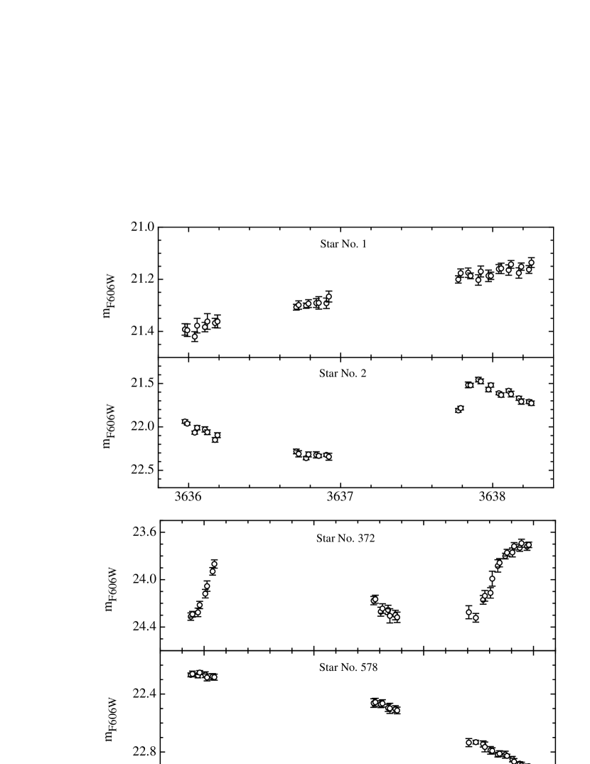
Figure 2: Unphased light curves for a sample of our variable stars with periods that are comparable to or longer than our observing window. The numbers refer to the stars in Tables 4 and 5.

Tables 2 and 3 list the individual F606W magnitudes of each variable at each epoch wherein 2 450 000 has been subtracted from the epoch value while Tables 4 and 5 list the candidate variables in our two fields along with their properties such as period, amplitude, and mean intensity-weighted magnitude. These stars fall into two broad categories. First, there are those that clearly show variability, but their periods are comparable to or longer than our observing window. These are referred to as ‘long period’ in Tables 4 and 5. There is also one candidate anomalous cepheid in our dataset, which is so indicated in Table 5. The second category includes stars that exhibit clear periodic variability with a period that is significantly shorter than our observing window but longer than 0.2d. These are the stars for which we can be confident of our periods. Some examples of stars with periods longer than our observing window are shown in Fig. 2 while Fig. 3 shows phased light curves of a number of contact and eclipsing binaries in our dataset. Figure 4 displays the phased light curves of all of the RR Lyrae variables for which we have derived periods.

All of the stars that exhibit RR Lyrae light curves also have apparent magnitudes in the range one would expect if they are at the distance of M31. Therefore, it is reasonable to assume that most if not all of these objects are RR Lyrae stars belonging to M31 and/or its environs. This assertion will become clearer when we compare the luminosity function (LF) of the non-variable stars with that of the RR Lyraes.

It should be noted that we are much less confident about the properties of the eclipsing and contact binaries that we have identified as compared with the RR Lyraes. This is because we know what period range to expect for the RR Lyraes ($\sim$0.25d to $\sim$0.90d), so that our observing window provides coverage of multiple cycles of variation for a given RR Lyrae star. In contrast, the periods of the eclipsing and contact binaries cannot be similarly constrained so it is difficult for us to ensure that our observing window is sufficient to derive the periods of these variables. As such, we have provided information for these stars (positions, periods, amplitudes, and magnitudes) so that future observers can confirm the nature of their variability, but we will not consider them further here. Instead, for the remainder of this paper, we will limit our discussion to the 681 RR Lyrae variables in our sample and what they reveal about the properties of the M31 system.

3.3 Light Curve Simulations

In order to characterize the possible biases in the derived periods of our variable star sample, we have performed simulations of our light curve fitting technique in the following manner. For the ab-type RR Lyraes, we selected one of the light curve templates (the results are insensitive to the actual ab-type template used) and produced artificial variables with a period range of 0.45 to 0.80 days and amplitudes between 0.3 and 1.3 mag. For the c-type RR Lyraes, a period range of 0.25 to 0.40 days and an amplitude range of 0.2 to 0.5 mag was used. One thousand variables were generated in each case and the mean photometric error at the level of the RR Lyraes was used to populate the light curves using the same observing window as the actual data. These simulated light curves were input into our template light curve fitting software. We are interested in comparing the input periods with the output periods in order to gauge any possible biases present in our analysis method.

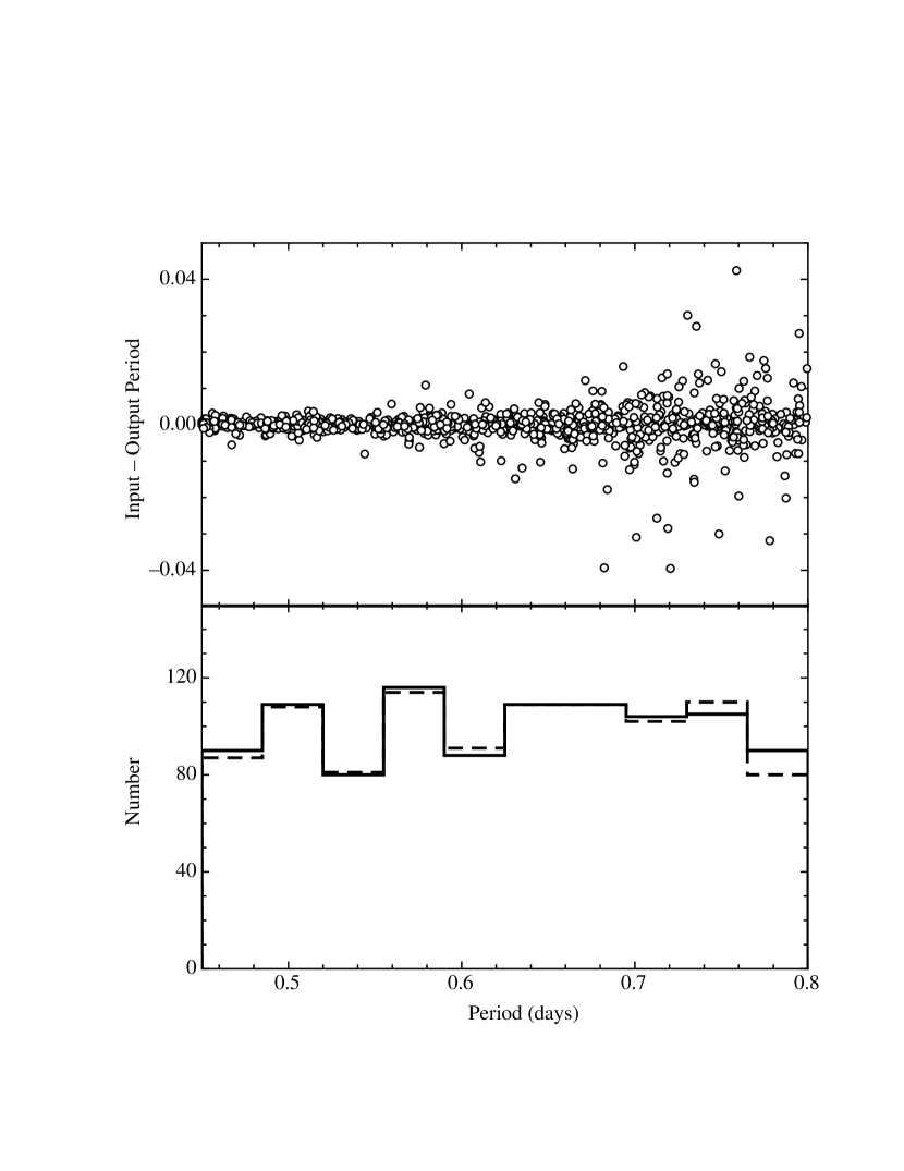
Figure 5: The results of the light curve simulations performed in order to characterize any biases in our period finding algorithm in the case of the RRab variables. The upper panel plots the variation of input minus recovered period while the lower panel plots the period distribution both as a function of period in days. The solid line is the input distribution while the dashed line represents the recovered one. These simulations suggest that the combination of the input data and the period-finding algorithm do not introduce significant biases in our derived periods.

Figures 5 (RRab) and 6 (RRc) show the result of these fits for Field 1 wherein the upper panel shows the mean difference between the input and output periods while the lower panel illustrates the differences in the period distributions. The result of the simulations for RR Lyraes in Field 2 are indistinguishable from those in Field 1. Of the 1000 ab-type RR Lyraes generated, none were mistaken for any other type of variable among the 10 light curve templates used in the fitting. For the c-type light curves, 2 of the 1000 generated variables were fit with a contact binary template. We find no significant biases in our determination of the periods for both types of RR Lyraes. As such, we will not apply any sort of correction to our derived periods. As for the errors in the period and amplitude determinations, these simulations suggest that an individual ab-type RR Lyrae has an error of $\pm$0.005 day and $\pm$0.044 mag, respectively. For a c-type RR Lyrae star, these error values are $\pm$0.001 day and $\pm$0.022 mag.

4 Results

4.1 Luminosity Functions

Figure 7 displays a comparison of the LFs of the nonvariable stars in the two fields. Both distributions feature a quick rise from brighter magnitudes to fainter ones with a pronounced peak at $m_{F606W}$$\sim$25.3 representing the core-helium burning horizontal branch (HB) stars. A sudden drop in both LFs at $m_{F606W}$$\sim$27.7 suggests the onset of significant incompleteness as the limit of the photometry is approached. The fact that the HB stars are more than 2 magnitudes brighter than this completeness threshold indicates that our sample of RR Lyrae variable candidates should not be adversely biased by photometric incompleteness.

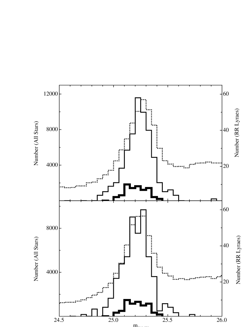
Figure 8: The luminosity functions (LFs) for the non-variable stars (dashed lines) compared with those of the RR Lyrae candidates (thin solid lines) in the two fields studied herein (see Table 1). The thicker solid lines represent the RR Lyrae stars from the study of Brown et al. (2004).

The two panels of Fig. 8 compare the LF of the nonvariable stars with those of the RR Lyraes in the two observed fields. We have used the intensity-weighted magnitudes listed in Tables 4 and 5 to construct these distributions. Gaussian fits to the regions around the RR Lyrae LF peaks yield $\langle$$m_{F606W}$$\rangle$$=25.20\pm 0.04$ for Field 1 and $\langle$$m_{F606W}$$\rangle$$=25.22\pm 0.04$ for Field 2, where the errors represent the standard error of the mean combined with the uncertainty in the photometric zeropoint added in quadrature. For the nonvariable stars, these peaks correspond to $\langle$$m_{F606W}$$\rangle$$=25.25\pm 0.04$ for Field 1 and $\langle$$m_{F606W}$$\rangle$$=25.23\pm 0.04$ for Field 2. The 1-$\sigma$ width of these distributions is $\sim$0.11 mag. These numbers suggest no significant difference in the mean magnitudes of the RR Lyraes and the nonvariable stars. This serves to confirm our assertion that most if not all of the variable stars in this magnitude range are RR Lyrae variables. In addition, when we combine the RR Lyrae variables from both fields, we find a mean magnitude of $m_{F606W}$$=25.21\pm 0.01$ on the VEGAmag system. The quoted uncertainty represents the standard error of the mean. When converted to the V-band using the mean offset for RR Lyraes in the middle of the instability strip from B2004 of $V-m_{F606W}$ = 0.08 $\pm$ 0.04, we derive $\langle$$V(RR)$$\rangle$$=25.29\pm 0.01$ (random) $\pm 0.05$ (systematic). This compares favorably with the value of $\langle$$V(RR)$$\rangle$$=25.30\pm 0.01$ based on the average for the ab-type and c-type RR Lyraes from the B2004 study (see Fig. 8). We note in passing that a Gaussian fit to the LF of the B2004 RR Lyraes yields a 1-$\sigma$ width of 0.12 mag, which is comparable to the value for the RR Lyraes in the present study.

4.2 Number Ratios

Of the 681 total RR Lyrae stars in our sample, 555 (267 in Field 1 and 288 in Field 2) are of the ab-type with the remainder being c-type (57 in Field 1 and 69 in Field 2). This leads to a ratio of $N_{c}/N_{abc}$=0.19$\pm$0.02, which is quite different than the value of $N_{c}/N_{abc}$=0.46$\pm$0.11 inferred from the B2004 data. Therefore, our samples of ab-type and c-type RR Lyraes are a factor of $\sim$2 greater and a factor of $\sim$2 less, respectively, than what we would expect based on the B2004 field. Taken at face value, this suggests that the old population in the environs of M31 exhibits different pulsation properties at 4–6 kpc as compared with 11 kpc.

To evaluate the validity of this assertion, we need to address the question of incompleteness in our sample of RR Lyraes. Are there significant numbers of RR Lyraes in our fields that we have failed to identify? We begin by noting that B2004 claim that their samples of c-type and ab-type RR Lyraes are complete and not significantly contaminated by dwarf cepheids. Therefore, we can gain some insight by comparing the amplitude distributions of the B2004 RR Lyrae variables with our sample as shown in Fig. 9. This comparison suggests that the amplitude distribution of the B2004 RR Lyraes are consistent with those of our sample. Application of the Kolmogorov-Smirnov test to these distributions confirms this suggestion. The fact that, at the low amplitude end, the two distributions are not substantially different argues that significant numbers of low amplitude RR Lyraes are not missing from our sample.

Another possibility to explain the differences in the $N_{c}/N_{abc}$ ratio between our fields and the one at 11 kpc is that our Field 1 data are significantly influenced by the stellar populations of M32 and not M31. In fact, we find $N_{c}/N_{abc}$=0.18$\pm$0.0.025 in Field 1 and $N_{c}/N_{abc}$=0.19$\pm$0.025 in Field 2, which are statistically indistinguishable from each other. In addition, the density of RR Lyrae variables and their period distributions are indistinguishable between fields 1 and 2. For example, for the ab-type variables, Field 1 exhibits a mean period of $\langle$$P_{ab}$$\rangle$$=0.553\pm 0.004$ while Field 2 shows $\langle$$P_{ab}$$\rangle$$=0.561\pm 0.005$. In the case of the c-type RR Lyraes, the analogous values are $\langle$$P_{c}$$\rangle$$=0.326\pm 0.005$ and $\langle$$P_{c}$$\rangle$$=0.327\pm 0.004$, respectively. These values suggests that both of our fields sample the regions around M31 and are minimally contaminated by M32 RR Lyraes.

If this difference in the $N_{c}/N_{abc}$ ratio between a radial distance of 11 kpc and 4–6 kpc in M31 is real, then it suggests that the RR Lyraes at 11 kpc are more akin to their brethren in Oosterhoff type II globular clusters while those at 4–6 kpc are more like RR Lyraes in Oosterhoff type I clusters. This is based on the fundings of Castellani et al. (2003) who examined the $N_{c}/N_{abc}$ ratio in Galactic globulars. They found that among the 12 clusters with 40 or more variables, $\langle$$N_{c}/N_{abc}$$\rangle$ = 0.37 for Oosterhoff II clusters and $\langle$$N_{c}/N_{abc}$$\rangle$ = 0.17 for those of Oosterhoff type I. These compare favorably with the values of $\langle$$N_{c}/N_{abc}$$\rangle$ = 0.46 for the 11 kpc field and $\langle$$N_{c}/N_{abc}$$\rangle$ = 0.19 for the 4–6 kpc field.

4.3 Periods, Amplitudes, and Metallicities

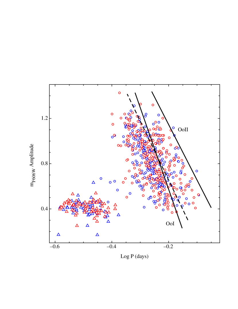
Figure 10: The Bailey Diagram for the RR Lyrae candidates in our fields. The open circles are the ab-type RR Lyraes while the open triangles represent the c-type variables. The color coding represents the field number with blue being stars observed in field 1 and red those found in field 2. This plot shows that, while the ab- and c-type RR Lyraes occupy their characteristic locations in this diagram, there is no significant difference between the RR Lyraes in the two observed fields. The dashed line shows the relation exhibited by the RRab stars in the field observed by Brown et al. (2004). The solid lines are the relations for Oosterhoff type I and II globular clusters from Clement (2000). These lines have been adjusted to account for the difference between an amplitude in the V-band and one in the F606W band.

The Bailey Diagram for our sample of RR Lyraes is shown in Fig. 10 where we plot the variables in the two fields using different colors. However, it is clear that they occupy the same regions of this diagram. The ab-type RR Lyrae variables are shown with open circles while the c-type stars are plotted as open triangles. The dashed line in Fig. 10 represents the relation exhibited by the RRab stars in the B2004 field. The solid lines are the relations for Oosterhoff I and II globular clusters from Clement (2000). These lines have been adjusted to account for the difference between an amplitude in the V-band and one in the F606W band. Interestingly, the B2004 RR Lyrae relation is closer to the OoI line even though the $N_{c}/N_{abc}$ ratio in the B2004 field is closer to that of OoII clusters. It is unclear why this should be the case.

The B2004 line appears to be offset compared with our data suggesting slightly shorter periods for the RRab variables in our fields. This behavior is further exemplified in Fig. 11 which shows the period distributions in the two fields compared with the mean periods of the ab- and c-type RR Lyraes from B2004. We find mean periods of $\langle$$P_{ab}$$\rangle$$=0.557\pm 0.003$ and $\langle$$P_{c}$$\rangle$$=0.327\pm 0.003$. For the B2004 field, these values are $\langle$$P_{ab}$$\rangle$$=0.594\pm 0.015$ and $\langle$$P_{c}$$\rangle$$=0.316\pm 0.007$. The mean periods of the c-type variables are statistically indistinguishable from each other but the ab-types in our fields exhibit a somewhat shorter period as compared with those in the B2004 fields.

It is well known that as the metallicity of ab-type RR Lyraes increases, their periods decrease (e.g. Sandage 1993; Layden 1995; Sarajedini et al. 2006). Thus, the period distribution of these stars (Fig. 11) can be converted to a metallicity distribution using equations derived by previous investigators. Using the data of Layden (2005, private communication) for 132 Galactic RR Lyraes in the solar neighborhood, Sarajedini et al. (2006) established a relation between period and metal abundance of the form

$$[Fe/H]=-3.43-7.82~{}Log~{}P_{ab}.$$ (1)

This equation does not take into account the amplitudes of the RR Lyraes even though, as Fig. 10 shows, there is a relation between amplitude and period for the ab-types. The work of Alcock et al. (2000) yielded a period-amplitude-metallicity relation of the form

$$[Fe/H]=-8.85[Log~{}P_{ab}+0.15A(V)]-2.60,$$ (2)

where $A(V)$ represents the amplitude in the V-band. We applied an 8% increase to the $m_{F606W}$ amplitudes to convert them to V-band values (B2004). Figure 12 shows the metallicity distribution function (MDF) for the ab-type RR Lyraes. The top panel compares the results obtained using equations (1) and (2) while the lower panel compares the MDFs for the two fields using Equation (2).

We see in the upper panel of Fig. 12 that, while the two MDFs exhibit very similar peak metallicities, the MDF generated using Eqn (2) displays a more prominent peak. This is representative of the fact that Eqn (2) accounts for the variation of period with amplitude as well as metallicity resulting in a cleaner abundance signature in the MDF. In the lower panel of Fig. 12, we see that the peaks of the RR Lyrae MDFs in our two fields differ by $\sim$0.1 dex; we find $\langle$[Fe/H]$\rangle$ = $-1.46\pm 0.03$ for Field 1 and $\langle$[Fe/H]$\rangle$ = $-1.54\pm 0.03$ for Field 2, where the errors represent standard errors of the mean. This difference is not statistically significant.

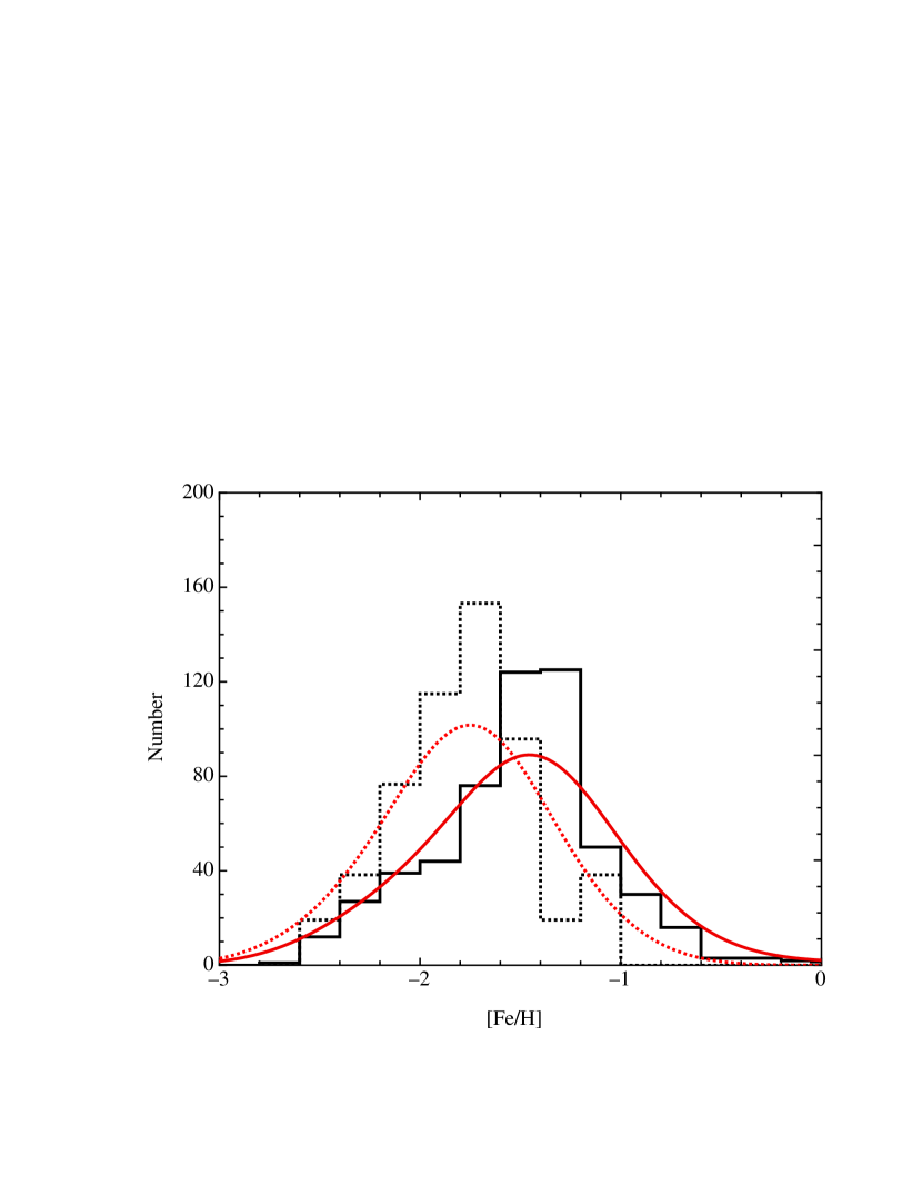
Figure 13: A comparison of the metallicity distribution function derived from the ab-type RR Lyraes from the present study (solid lines) and those from the Brown et al. (2004) study (dotted lines). The latter has been scaled to match the number of ab-type RR Lyraes in our two fields. Both binned and generalized histograms are shown.

Combining the RR Lyraes in the two fields yields the MDF shown as the solid line in Fig. 13, wherein the binned and generalized histograms are shown. The latter has been constructed using an error of 0.31 dex per star (Alcock et al. 2000). The peak metallicity for our sample of ab-type RR Lyraes is then $\langle$[Fe/H]$\rangle$=$-1.50\pm 0.02$ where the error is the standard error of the mean. The systematic error of this measurement is likely to be closer to $\sim$0.3 dex. The dotted distributions in Fig. 13 are the binned and generalized histograms for the RRab stars in the sample of B2004 scaled to the same number of ab-type RR Lyraes as in our fields. The peak abundance of this MDF is $\langle$[Fe/H]$\rangle$=$-1.77\pm 0.06$.

There are three observations we can make regarding the appearance of Fig. 13. First, it would seem that the errors on the individual metallicity measurements are significant enough to overwhelm any fine-structure that may be present in the two MDFs. That is to say, both MDFs look essentially like normal distributions. Second, since we have applied the same transformation from period to metallicity to both sets of RR Lyraes, we can assert with significant statistical certainty that the mean metal abundance of the RR Lyraes in the B2004 field is lower than that of the RR Lyraes in our two fields. This difference amounts to $\Delta$$[Fe/H]=0.27\pm 0.06$ and reflects back on the period shift seen in the Bailey Diagram shown in Fig. 10. Third, there are a small but non-negligible number of ab-type RR Lyraes with metallicities above $[Fe/H]$$\sim$-1 that are not seen in the B2004 field. Given the fact that our field is closer to the central regions of M31 as compared with the B2004, it is possible that these metal-rich RR Lyraes could belong to the bulge or disk of M31. We return to this point in the next section.

One last point needs to be addressed before leaving this section and that is concerned with the M31 distance implied by the RR Lyraes in our sample. Using the relation advocated by Chaboyer (1999) of $M_{V}(RR)=0.23[Fe/H]+0.93$ and a reddening of $E(B-V)=0.08\pm 0.03$ (Schlegel et al. 1998), we find a distance modulus of $(m-M)_{0}=24.46\pm 0.11$. This is consistent with the B2004 value and a number of previous determinations.

5 Discussion

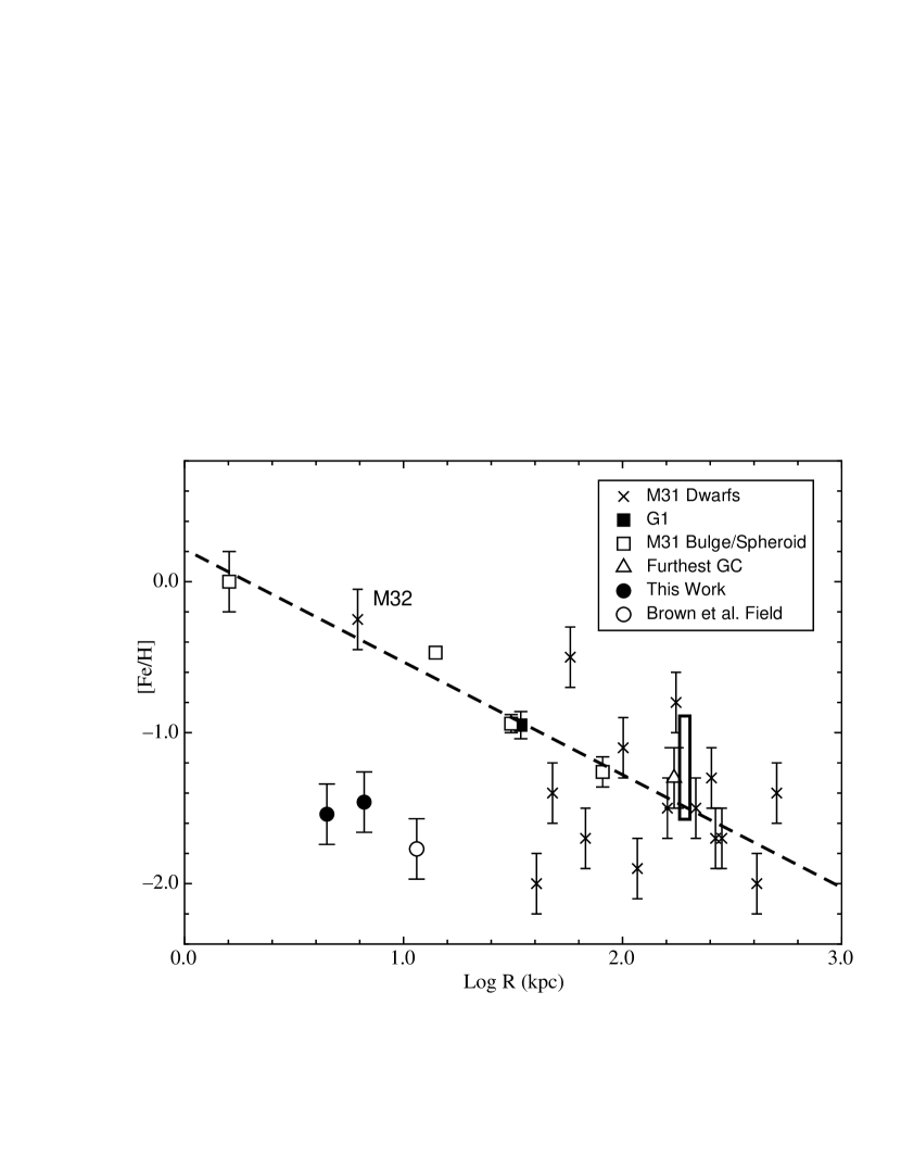
Figure 14: A plot of the variation of metal abundance with projected distance from the center of M31. Our results are shown by the filled circles while the mean metallicity of the RR Lyraes studied by Brown et al. (2004) is indicated by the open circle. The inner most open square represents the bulge abundance measured by Sarajedini & Jablonka (2006). The remaining open squares are the bulge/halo points from the work of Kalirai et al. (2006). The dashed line is the least squares fit to these data with a slope of –0.75 $\pm$ 0.11. The crosses represent the dwarf galaxies surrounding M31 from the work of Grebel et al. (2003) and Koch & Grebel (2006) whereas the abundance of M32 is taken from Grillmair et al. (1996). The filled square is the well-known massive globular cluster G1 studied by Meylan et al. (2001). The open triangle is the furthest known globular cluster in M31 discovered by Martin et al. (2006). For completeness, the boxed region shows the location of the halo globular clusters in M33 from the work of Sarajedini et al. (2000). All of these points have been scaled to an M31 distance of $(m-M)_{0}$ = 24.43.

We now seek to place our RR Lyrae abundance results within the broader context of the projected radial metallicity distribution of various populations in the environs of M31. Figure 14 shows this information for a range of stellar populations in and around M31. The metallicities for the RR Lyraes in the two fields considered herein are shown by the filled circles while the open circle represents the RR Lyraes in the B2004 field. The inner-most point is the bulge metallicity from the work of Sarajedini & Jablonka (2005), while the remaining open squares are the bulge/halo points from the work of Kalirai et al. (2006) as shown in their Table 3. The dashed line is the least squares fit to the open squares with a slope of $-0.75\pm 011$. The other points represent the dwarf spheroidal companions to M31 (crosses, Grebel et al. 2003; Koch & Grebel 2006), the globular cluster G1 (filled square, Meylan et al. 2001), and the furthest globular cluster in M31 (open triangle, Martin et al. 2006). Note that we have adopted the mean metallicity of M32 from the work of Grillmair et al. (1996). The elongated rectangle represents the locations of the halo globular clusters in M33 from Sarajedini et al. (2000). All of these values are based on a distance of $(m-M)_{o}=24.43$ (770 kpc) for M31. In cases where an error in the metallicity is not available, we have adopted a value of $\pm$0.2 dex.

We see in Fig. 14 a clear representation of the notion that the halo population in M31 does not begin to dominate until a galactocentric distance of $\sim$30 kpc, as suggested by a number of authors (Guhathakurta et al. 2005; Irwin et al. 2005; Kalirai et al. 2006; Koch et al. 2007). At this location, we see a transition region between the globular cluster G1 which is consistent with the inner-spheroid metallicity gradient (dashed line) and the dwarf spheroidal galaxies which show no relation between abundance and galactocentric distance. In this sense, it would appear that the RR Lyrae populations in our field and that of B2004 follow the trend outlined by the stellar populations outside of $\sim$30 kpc. This suggests that the RR Lyraes at these locations are probably members of the M31 halo rather than its bulge suggesting that the halo can be studied as close as 4 kpc from the center of M31 by focusing on the RR Lyraes.

6 Summary and Conclusions

We have presented F606W ($\sim$V) observations from the HST archive taken with the Advanced Camera for Surveys of two fields located 4-6 kpc from the center of M31. In these regions, we identify 752 variable stars of which 681 are likely to be bona fide RR Lyraes. From the properties of these stars, we draw the following conclusions.

1) The mean magnitude of the RR Lyrae stars is $\langle$$V$$\rangle$$=25.29\pm 0.05$ where the uncertainty combines both the random and systematic errors. This is in good agreement with the results of Brown et al. (2004)

2) The ratio of c-type RR Lyraes to all types is reminiscent of the RR Lyraes in Oosterhoff type I globular clusters in the Milky Way. This ratio is significantly different than the Brown et al. (2004) field at 11 kpc from the center of M31 wherein this ratio is closer to that of Oosterhoff II clusters.

3) When the periods and amplitudes of the ab-type RR Lyraes in our sample are interpreted in terms of metallicity, we find the metallicity distribution function to be indistinguishable from a Gaussian with a peak at $\langle$[Fe/H]$\rangle$=$-1.50\pm 0.02$, where the error is the standard error of the mean. The same analysis applied to the Brown et al. (2004) RR Lyraes yields a peak of $\langle$[Fe/H]$\rangle$=$-1.77\pm 0.06$.

4) Using the RR Lyrae luminosity - metallicity relation advocated by Chaboyer (1999) and a reddening of $E(B-V)=0.08\pm 0.03$, we find a distance modulus of $(m-M)_{0}=24.46\pm 0.11$ for M31.

5) We examine the radial metallicity gradient in the environs of M31 using published values for the bulge and halo of M31 as well as the abundances of the dwarf spheroidal companions and globular clusters of M31. In this context, despite the relative proximity of the RR Lyraes in the present study to the center of M31, their metal abundance is more reminiscent of a halo population than a bulge or disk. Therefore, by using the RR Lyraes as a proxy, the halo can be studied as close as 4 kpc from the center of M31.

Table 1: Observing Log

Field	RA (J2000)	Decl. (J2000)	Starting Date	Datasets	Filter	Exp Time	HJD Range (+2 453 000)
1	00 42 41.2	40 46 38	September 22, 2005	J9H905, J9H906,	F606W	16 $\times$ 1136s,	635.97 to 638.25
				J9H907, J9H908		16 $\times$ 1177s
2	00 43 20.8	40 57 25	February 9, 2006	J9H913, J9H914,	F606W	16 $\times$ 1136s,	775.88 to 778.96
				J9H915, J9H916		16 $\times$ 1177s

Table 2: Raw Light Curves Field 1

Epoch	001 Mag	001 Err	002 Mag	002 Err	003 Mag	003 Err	004 Mag	004 Err	005 Mag	005 Err
3635.97534180	21.414	0.022	21.960	0.021	24.033	0.033	24.782	0.059	24.639	0.049
3635.99096680	21.417	0.024	21.984	0.017	24.023	0.033	24.826	0.052	24.664	0.049
3636.04003906	21.442	0.019	22.088	0.018	24.024	0.052	24.967	0.065	24.699	0.044
3636.05566406	21.400	0.028	22.032	0.025	24.011	0.021	$\cdots$	$\cdots$	24.650	0.052
3636.10693359	21.405	0.018	22.051	0.030	24.016	0.051	24.750	0.034	24.604	0.045
3636.12304688	21.384	0.030	22.083	0.027	24.013	0.042	24.582	0.038	24.585	0.046
3636.17358398	21.390	0.018	22.171	0.027	23.998	0.043	$\cdots$	$\cdots$	24.556	0.039
3636.18969727	21.384	0.025	22.118	0.028	$\cdots$	$\cdots$	$\cdots$	$\cdots$	24.607	0.056
3636.70800781	21.329	0.011	22.305	0.027	24.050	0.059	24.706	0.039	24.890	0.037
3636.72363281	21.321	0.016	22.332	0.036	24.036	0.036	24.755	0.031	24.799	0.042
3636.77294922	21.323	0.010	22.382	0.019	$\cdots$	$\cdots$	24.853	0.044	24.617	0.022
3636.78833008	21.315	0.015	22.339	0.029	24.037	0.035	24.846	0.048	24.552	0.049
3636.83959961	21.313	0.017	22.344	0.035	24.057	0.045	24.784	0.029	24.594	0.055
3636.85571289	21.312	0.024	22.356	0.019	24.018	0.056	24.754	0.058	24.618	0.049
3636.90625000	21.314	0.020	22.344	0.018	24.074	0.043	24.673	0.053	24.619	0.037
3636.92236328	21.288	0.021	22.366	0.040	24.061	0.036	24.554	0.033	24.523	0.054
3637.77368164	21.222	0.014	21.832	0.022	23.992	0.040	24.629	0.037	24.619	0.025
3637.78930664	21.198	0.016	21.805	0.021	24.012	0.022	24.553	0.036	24.640	0.026
3637.83862305	21.197	0.018	21.538	0.033	23.949	0.030	24.672	0.039	24.643	0.040
3637.85424805	21.209	0.011	21.542	0.023	23.994	0.037	24.704	0.048	24.649	0.045
3637.90551758	21.225	0.020	21.477	0.027	23.980	0.034	24.932	0.071	24.646	0.098
3637.92163086	21.192	0.021	21.498	0.028	23.977	0.030	24.875	0.050	24.617	0.062
3637.97216797	21.208	0.022	21.591	0.026	$\cdots$	$\cdots$	24.882	0.026	24.606	0.087
3637.98803711	21.208	0.014	21.541	0.023	23.987	0.031	24.841	0.044	$\cdots$	$\cdots$
3638.04028320	21.183	0.017	21.634	0.018	24.000	0.025	24.764	0.032	24.669	0.042
3638.05566406	21.180	0.020	21.655	0.025	24.007	0.025	24.673	0.050	24.594	0.071
3638.10498047	21.186	0.020	21.606	0.021	24.000	0.036	24.594	0.038	24.914	0.036
3638.12060547	21.165	0.015	21.644	0.033	24.063	0.022	24.587	0.026	25.073	0.057
3638.17187500	21.198	0.020	21.692	0.024	24.060	0.034	24.648	0.041	25.115	0.047
3638.18798828	21.173	0.014	21.730	0.031	24.031	0.043	24.639	0.028	25.236	0.091
3638.23852539	21.184	0.015	21.732	0.022	24.043	0.073	24.754	0.025	24.946	0.068
3638.25463867	21.158	0.019	21.750	0.026	24.086	0.035	24.760	0.038	24.909	0.035

Table 3: Raw Light Curves Field 2

Epoch	366 Mag	366 Err	367 Mag	367 Err	368 Mag	368 Err	369 Mag	369 Err	370 Mag	370 Err
3775.87866211	21.896	0.034	22.464	0.029	22.360	0.038	$\cdots$	$\cdots$	23.676	0.023
3775.89428711	21.955	0.031	22.409	0.050	22.387	0.038	23.583	0.025	23.667	0.036
3775.94409180	21.901	0.024	22.388	0.041	22.347	0.028	23.624	0.024	23.597	0.026
3775.95971680	21.885	0.035	22.443	0.029	22.342	0.038	23.626	0.026	23.664	0.030
3776.01098633	21.930	0.028	22.417	0.043	22.347	0.029	23.686	0.027	23.607	0.020
3776.02685547	21.881	0.034	22.400	0.032	22.387	0.032	23.689	0.036	23.579	0.036
3776.07763672	21.886	0.027	22.384	0.032	22.391	0.035	23.716	0.026	23.584	0.033
3776.09350586	21.914	0.019	22.323	0.063	22.332	0.028	23.688	0.037	23.592	0.022
3777.54418945	21.748	0.044	22.178	0.041	22.234	0.034	23.806	0.070	23.671	0.035
3777.55957031	21.693	0.035	22.174	0.054	22.178	0.030	23.807	0.063	23.741	0.034
3777.60913086	21.706	0.034	22.179	0.049	22.159	0.029	23.836	0.053	23.740	0.041
3777.62475586	21.722	0.043	22.174	0.040	22.053	0.060	23.872	0.066	23.707	0.034
3777.67602539	21.692	0.053	22.166	0.045	22.150	0.029	23.863	0.029	23.698	0.029
3777.69189453	21.711	0.063	22.149	0.033	22.140	0.036	23.888	0.040	23.719	0.042
3777.74243164	21.710	0.060	22.160	0.025	22.158	0.028	23.858	0.029	23.672	0.047
3777.75854492	21.679	0.049	22.156	0.041	22.152	0.029	23.855	0.033	23.664	0.023
3778.41113281	21.662	0.028	22.085	0.020	22.113	0.024	23.397	0.020	23.635	0.055
3778.47485352	21.656	0.032	22.074	0.020	22.128	0.033	23.454	0.029	23.702	0.061
3778.54150391	21.652	0.033	22.067	0.026	22.113	0.035	23.553	0.036	23.899	0.056
3778.55712891	21.636	0.032	22.065	0.024	22.097	0.023	23.515	0.026	23.905	0.059
3778.60839844	21.589	0.043	22.055	0.034	22.081	0.035	23.567	0.030	23.981	0.032
3778.62451172	21.614	0.025	22.052	0.039	22.085	0.033	23.594	0.029	23.941	0.027
3778.67504883	21.618	0.032	22.055	0.035	22.087	0.030	23.584	0.023	23.783	0.038
3778.69116211	21.599	0.044	22.045	0.035	22.059	0.042	23.632	0.034	23.834	0.034
3778.74340820	21.592	0.028	22.056	0.038	22.077	0.036	23.671	0.023	23.735	0.026
3778.75903320	21.609	0.034	22.041	0.031	22.054	0.059	23.721	0.025	23.815	0.040
3778.80786133	21.600	0.027	22.030	0.022	22.055	0.036	23.723	0.018	23.653	0.020
3778.82348633	21.594	0.028	22.053	0.036	22.016	0.036	23.746	0.020	23.687	0.031
3778.87475586	21.581	0.029	22.049	0.045	22.038	0.031	23.779	0.029	23.656	0.021
3778.89086914	21.608	0.025	22.047	0.039	22.029	0.032	23.814	0.030	23.659	0.020
3778.94140625	21.597	0.013	22.040	0.041	22.044	0.023	23.835	0.024	23.638	0.019
3778.95751953	21.597	0.025	22.032	0.038	22.045	0.034	23.845	0.029	23.667	0.028

Table 4: Field 1 Variable Stars

Star ID	RA (J2000)	Dec (J2000)	Period (days)	$m_{F606W}$ Amplitude	$\langle$$m_{F606W}$$\rangle$	Type
1	0 42 38.35	40 47 8.3	1.551	0.301	21.337	long period
2	0 42 41.92	40 45 19.1	2.559	0.919	22.070	long period
3	0 42 37.94	40 45 18.9	1.408	0.100	24.029	long period
4	0 42 34.90	40 46 4.3	0.387	0.288	24.712	RRc
5	0 42 42.82	40 45 23.6	1.561	0.490	24.685	Eclipsing
6	0 42 34.49	40 46 29.0	1.400	0.246	24.758	Contact
7	0 42 41.61	40 46 7.4	0.660	0.725	24.877	RRab
8	0 42 42.42	40 44 59.8	1.539	0.160	24.820	long period
9	0 42 43.09	40 44 59.0	0.508	0.575	24.859	RRab
10	0 42 36.11	40 47 13.9	2.188	0.130	24.918	long period
11	0 42 43.88	40 44 41.7	0.642	0.825	25.034	RRab
12	0 42 38.30	40 45 58.6	0.743	0.599	24.930	RRab
13	0 42 31.65	40 46 53.8	0.749	0.403	24.988	Contact
14	0 42 37.81	40 45 32.7	0.682	0.937	24.952	RRab
15	0 42 41.33	40 45 18.6	0.697	0.718	25.062	RRab
16	0 42 35.83	40 46 12.0	0.342	0.472	25.025	RRc
17	0 42 44.37	40 45 0.2	0.708	0.803	24.975	RRab
18	0 42 40.85	40 45 1.0	0.488	0.635	25.019	RRab
19	0 42 35.77	40 46 44.1	0.744	0.444	25.086	RRab
20	0 42 38.05	40 46 57.9	0.376	0.377	25.073	RRc
21	0 42 46.29	40 46 3.5	0.805	0.523	25.061	RRab
22	0 42 39.16	40 45 55.6	0.339	0.357	25.095	RRc
23	0 42 33.52	40 46 16.4	0.365	0.459	25.121	RRc
24	0 42 34.23	40 47 28.1	0.611	0.693	25.078	RRab
25	0 42 46.08	40 45 16.1	0.705	0.427	25.154	RRab
26	0 42 34.51	40 47 11.4	0.641	0.616	25.049	RRab
27	0 42 37.99	40 46 49.8	0.555	0.669	25.103	RRab
28	0 42 43.53	40 45 38.6	0.596	0.827	25.117	RRab
29	0 42 43.41	40 46 30.1	0.497	0.991	25.200	RRab
30	0 42 41.43	40 46 10.7	0.328	0.440	25.096	RRc
31	0 42 42.05	40 46 7.1	0.567	0.937	25.138	RRab
32	0 42 43.80	40 46 15.3	0.597	0.633	25.191	RRab
33	0 42 39.84	40 45 50.0	0.355	0.356	25.097	RRc
34	0 42 40.83	40 45 22.0	0.618	0.719	25.186	RRab
35	0 42 42.73	40 45 18.2	0.531	0.749	25.215	RRab
36	0 42 42.68	40 44 44.3	0.689	0.504	25.207	RRab
37	0 42 35.22	40 46 24.8	0.502	1.020	25.130	RRab
38	0 42 44.21	40 45 3.9	0.332	0.413	25.143	RRc
39	0 42 47.25	40 45 21.1	0.627	0.650	25.240	RRab
40	0 42 32.79	40 46 7.9	0.537	0.928	25.079	RRab
41	0 42 45.25	40 45 0.3	0.582	1.016	25.107	RRab
42	0 42 36.42	40 46 1.4	0.648	0.491	25.174	RRab
43	0 42 38.30	40 45 14.6	0.351	0.461	25.172	RRc
44	0 42 42.33	40 46 14.9	0.494	0.967	25.187	RRab
45	0 42 44.21	40 45 44.0	0.545	0.506	25.216	RRab
46	0 42 34.14	40 47 22.1	0.560	0.782	25.213	RRab
47	0 42 31.11	40 46 9.8	0.544	1.050	25.136	RRab
48	0 42 35.42	40 46 32.0	0.488	0.789	25.260	RRab
49	0 42 42.47	40 45 21.0	0.308	0.450	25.185	RRc
50	0 42 36.52	40 45 53.3	0.445	1.122	25.212	RRab
51	0 42 42.84	40 46 18.7	0.680	0.478	25.245	RRab
52	0 42 33.73	40 46 28.0	0.517	0.415	25.199	RRab
53	0 42 44.24	40 46 12.4	0.378	0.326	25.182	RRc
54	0 42 47.19	40 45 51.7	0.522	0.936	25.238	RRab
55	0 42 44.64	40 46 22.2	0.500	0.949	25.143	RRab
56	0 42 47.40	40 45 54.5	0.611	0.479	25.260	RRab
57	0 42 42.89	40 45 52.3	0.578	0.627	25.150	RRab
58	0 42 38.77	40 45 32.4	0.364	0.428	25.177	RRc
59	0 42 47.21	40 45 46.8	0.589	0.649	25.204	RRab
60	0 42 40.82	40 46 40.0	0.698	0.586	25.187	RRab
61	0 42 34.15	40 47 15.2	0.508	0.735	25.156	RRab
62	0 42 36.32	40 46 42.2	0.564	0.784	25.241	RRab
63	0 42 31.84	40 46 48.9	0.583	0.479	25.316	RRab
64	0 42 45.53	40 45 2.3	0.550	0.824	25.222	RRab
65	0 42 46.68	40 45 33.8	0.365	0.388	25.212	RRc
66	0 42 45.53	40 46 13.8	0.503	0.605	25.245	RRab
67	0 42 34.91	40 46 22.5	0.590	0.531	25.313	RRab
68	0 42 38.65	40 45 52.5	0.316	0.403	25.251	RRc
69	0 42 43.64	40 45 49.7	0.566	0.857	25.135	RRab
70	0 42 42.74	40 46 2.6	0.527	0.780	25.276	RRab
71	0 42 33.70	40 46 14.0	0.524	0.721	25.205	RRab
72	0 42 44.27	40 46 19.7	0.318	0.384	25.256	RRc
73	0 42 44.46	40 45 35.5	0.619	0.500	25.333	RRab
74	0 42 46.17	40 46 5.4	0.340	0.431	25.231	RRc
75	0 42 36.52	40 46 44.6	0.303	0.457	25.275	RRc
76	0 42 40.85	40 45 5.1	0.298	0.453	25.273	RRc
77	0 42 35.96	40 47 7.3	0.347	0.382	25.289	RRc
78	0 42 46.84	40 45 39.2	0.610	0.595	25.323	RRab
79	0 42 41.15	40 44 55.0	0.337	0.500	25.231	RRc
80	0 42 34.11	40 47 39.8	0.577	0.583	25.246	RRab
81	0 42 37.41	40 46 28.7	0.515	1.085	25.252	RRab
82	0 42 33.80	40 47 10.5	0.588	0.789	25.235	RRab
83	0 42 44.88	40 44 36.5	0.452	1.133	25.279	RRab
84	0 42 39.82	40 46 54.6	0.583	1.166	25.186	RRab
85	0 42 35.71	40 46 38.3	0.556	0.711	25.243	RRab
86	0 42 33.93	40 47 35.0	0.572	0.669	25.293	RRab
87	0 42 41.91	40 46 2.8	0.334	0.418	25.264	RRc
88	0 42 46.42	40 45 58.8	0.557	0.611	25.249	RRab
89	0 42 42.72	40 44 52.4	0.597	0.605	25.313	RRab
90	0 42 40.66	40 44 57.6	0.569	0.662	25.289	RRab
91	0 42 34.57	40 46 20.9	0.540	0.663	25.312	RRab
92	0 42 40.56	40 45 25.1	0.299	0.383	25.283	RRc
93	0 42 34.05	40 47 20.5	0.585	1.103	25.144	RRab
94	0 42 42.01	40 46 1.6	0.540	0.748	25.280	RRab
95	0 42 46.18	40 46 10.0	0.491	0.896	25.290	RRab
96	0 42 36.45	40 45 36.1	0.504	0.871	25.300	RRab
97	0 42 42.89	40 45 2.6	0.277	0.415	25.306	RRc
98	0 42 46.78	40 46 4.9	0.567	0.795	25.259	RRab
99	0 42 38.40	40 45 12.6	0.562	0.712	25.279	RRab
100	0 42 42.22	40 46 13.0	0.565	0.943	25.333	RRab
101	0 42 34.34	40 45 43.4	0.559	0.467	25.371	RRab
102	0 42 33.73	40 46 47.3	0.471	0.809	25.243	RRab
103	0 42 43.19	40 45 0.2	0.604	0.792	25.218	RRab
104	0 42 39.80	40 46 27.9	0.553	1.010	25.327	RRab
105	0 42 40.80	40 45 5.3	0.519	0.916	25.374	RRab
106	0 42 38.06	40 47 5.8	0.545	0.902	25.273	RRab
107	0 42 46.21	40 45 25.8	0.473	1.146	25.363	RRab
108	0 42 32.59	40 46 53.0	0.512	0.946	25.479	RRab
109	0 42 43.02	40 45 29.8	0.607	0.442	25.318	RRab
110	0 42 38.26	40 45 16.2	0.329	0.344	25.350	RRc
111	0 42 41.85	40 46 21.4	0.540	0.746	25.314	RRab
112	0 42 43.66	40 46 25.8	0.270	0.393	25.384	RRc
113	0 42 41.74	40 46 30.2	0.534	0.768	25.387	RRab
114	0 42 35.06	40 46 1.6	0.548	0.779	25.349	RRab
115	0 42 44.44	40 44 46.7	0.584	0.740	25.316	RRab
116	0 42 36.10	40 46 34.8	0.588	0.612	25.307	RRab
117	0 42 32.46	40 46 14.4	0.591	0.617	25.324	RRab
118	0 42 33.59	40 47 1.3	0.547	0.502	25.403	RRab
119	0 42 39.91	40 46 30.2	0.494	1.095	25.442	RRab
120	0 42 34.26	40 46 22.4	0.481	1.016	25.331	RRab
121	0 42 39.35	40 47 0.6	0.548	0.924	25.464	RRab
122	0 42 36.65	40 46 43.8	0.533	1.035	25.390	RRab
123	0 42 43.62	40 44 50.5	0.469	1.129	25.461	RRab
124	0 42 36.05	40 46 53.7	0.531	1.080	25.428	RRab
125	0 42 36.95	40 46 49.1	0.507	0.807	25.504	RRab
126	0 42 46.13	40 45 24.5	0.511	0.850	25.429	RRab
127	0 42 44.55	40 45 21.3	0.612	0.531	25.390	RRab
128	0 42 32.50	40 46 36.2	0.502	0.982	25.517	RRab
129	0 42 47.76	40 45 43.0	0.471	0.948	25.444	RRab
130	0 42 36.63	40 47 9.2	0.669	0.859	25.273	RRab
131	0 42 34.65	40 46 57.9	0.502	1.051	25.484	RRab
132	0 42 41.78	40 44 52.7	0.484	0.824	25.496	RRab
133	0 42 33.24	40 46 57.0	0.393	0.635	25.569	RRab
134	0 42 44.75	40 45 23.5	0.461	1.232	25.419	RRab
135	0 42 31.51	40 46 27.7	1.776	1.221	25.659	Eclipsing
136	0 42 38.41	40 46 22.4	1.747	0.516	25.642	Eclipsing
137	0 42 42.18	40 45 36.2	0.408	1.049	25.548	RRab
138	0 42 44.46	40 45 19.8	1.056	0.788	25.736	Contact
139	0 42 35.92	40 46 0.5	0.474	1.025	25.919	RRab
140	0 42 37.19	40 47 7.3	1.480	0.751	26.322	Contact
141	0 42 45.35	40 45 22.7	1.311	0.765	26.480	Eclipsing
142	0 42 34.47	40 46 44.5	1.597	0.945	26.490	Contact
143	0 42 40.89	40 47 19.3	2.061	0.252	22.197	long period
144	0 42 44.45	40 47 47.6	1.599	0.345	23.035	long period
145	0 42 37.88	40 48 6.3	1.556	0.505	23.412	long period
146	0 42 36.93	40 48 28.6	2.210	0.659	23.639	long period
147	0 42 38.51	40 48 39.3	1.389	0.339	23.843	long period
148	0 42 40.86	40 48 41.8	1.696	0.974	23.955	long period
149	0 42 45.30	40 48 0.8	1.117	0.375	24.108	Eclipsing
150	0 42 44.36	40 47 59.8	1.724	0.423	24.171	long period
151	0 42 44.30	40 47 45.7	0.354	0.170	24.354	RRc
152	0 42 42.98	40 48 2.6	0.486	0.646	24.585	RRab
153	0 42 37.88	40 48 55.3	0.656	1.117	24.998	RRab
154	0 42 39.50	40 49 3.8	1.344	0.535	24.712	Eclipsing
155	0 42 40.13	40 47 44.9	0.670	0.879	24.966	RRab
156	0 42 46.21	40 48 16.4	0.645	0.606	24.932	RRab
157	0 42 41.28	40 47 40.4	0.562	0.749	24.858	RRab
158	0 42 45.14	40 46 35.0	0.792	0.735	24.882	RRab
159	0 42 48.57	40 46 45.5	0.343	0.632	24.943	RRc
160	0 42 48.04	40 47 9.4	0.439	0.993	24.922	RRab
161	0 42 50.25	40 47 16.6	0.682	0.820	24.917	RRab
162	0 42 45.20	40 48 5.4	0.611	0.815	24.843	RRab
163	0 42 43.23	40 47 14.6	0.698	0.735	25.047	RRab
164	0 42 48.14	40 47 58.5	0.684	0.818	24.933	RRab
165	0 42 35.85	40 48 24.1	1.529	1.403	25.236	Contact
166	0 42 42.79	40 47 27.4	0.386	0.461	24.986	RRab
167	0 42 43.38	40 47 56.2	0.594	0.550	24.968	RRab
168	0 42 38.36	40 48 37.2	0.589	0.648	25.039	RRab
169	0 42 46.24	40 48 0.3	0.693	0.587	25.017	RRab
170	0 42 47.60	40 46 9.5	0.420	0.346	24.969	RRc
171	0 42 40.38	40 47 2.6	0.332	0.352	25.034	RRc
172	0 42 43.42	40 47 26.2	0.558	0.616	24.985	RRab
173	0 42 37.69	40 47 46.5	0.600	0.841	25.087	RRab
174	0 42 47.19	40 48 5.4	0.364	0.669	24.977	RRab
175	0 42 47.95	40 46 44.7	0.620	0.903	25.082	RRab
176	0 42 42.07	40 47 25.4	0.751	0.643	25.155	RRab
177	0 42 48.49	40 47 56.2	0.630	0.688	25.146	RRab
178	0 42 37.76	40 48 32.9	0.530	0.837	25.109	RRab
179	0 42 43.18	40 46 39.2	0.604	0.792	25.158	RRab
180	0 42 40.13	40 48 32.2	0.559	0.904	25.098	RRab
181	0 42 48.47	40 47 12.5	0.559	0.821	25.117	RRab
182	0 42 47.53	40 46 26.5	0.607	0.664	25.142	RRab
183	0 42 38.49	40 47 37.1	0.613	0.501	25.089	RRab
184	0 42 40.61	40 48 48.2	0.601	0.605	25.165	RRab
185	0 42 39.71	40 47 21.6	0.417	0.567	25.156	RRab
186	0 42 40.26	40 48 6.0	0.541	0.678	25.107	RRab
187	0 42 34.79	40 47 42.9	1.560	1.827	25.335	Contact
188	0 42 44.24	40 46 33.6	0.656	0.482	25.126	RRab
189	0 42 48.53	40 47 59.8	0.553	0.712	25.143	RRab
190	0 42 41.29	40 48 20.9	0.526	0.805	25.155	RRab
191	0 42 46.97	40 46 37.7	0.590	0.697	25.219	RRab
192	0 42 40.18	40 48 45.9	0.570	1.062	25.064	RRab
193	0 42 39.23	40 49 5.4	0.327	0.252	25.111	RRc
194	0 42 46.49	40 47 31.2	0.547	0.631	25.170	RRab
195	0 42 48.20	40 47 12.8	0.814	0.232	25.146	long period
196	0 42 41.44	40 48 47.8	0.345	0.373	25.084	RRc
197	0 42 45.64	40 46 32.5	0.589	0.599	25.169	RRab
198	0 42 36.65	40 47 45.7	0.491	1.010	25.093	RRab
199	0 42 44.01	40 48 6.4	0.610	0.467	25.210	RRab
200	0 42 34.62	40 47 49.9	0.604	0.629	25.246	RRab
201	0 42 46.25	40 48 6.7	0.583	0.601	25.139	RRab
202	0 42 47.12	40 47 35.5	0.535	0.740	25.092	RRab
203	0 42 52.45	40 47 6.2	0.546	0.811	25.216	RRab
204	0 42 44.27	40 47 3.3	0.357	0.455	25.090	RRc
205	0 42 37.55	40 48 9.0	0.471	0.918	25.030	RRab
206	0 42 39.73	40 48 54.6	0.590	0.880	25.232	RRab
207	0 42 39.18	40 49 0.1	0.277	0.410	25.168	RRc
208	0 42 42.72	40 47 24.4	0.384	0.339	25.137	RRc
209	0 42 49.76	40 47 3.4	0.380	0.369	25.154	RRc
210	0 42 37.62	40 47 23.3	0.361	0.384	25.152	RRc
211	0 42 37.66	40 48 55.6	0.665	0.935	25.120	RRab
212	0 42 47.17	40 47 32.7	0.568	0.919	25.143	RRab
213	0 42 50.28	40 47 34.1	0.516	0.923	25.217	RRab
214	0 42 41.64	40 47 44.6	0.729	0.491	25.151	RRab
215	0 42 41.71	40 48 38.3	0.481	0.886	25.126	RRab
216	0 42 46.61	40 47 13.5	0.582	1.230	25.041	RRab
217	0 42 40.65	40 48 36.8	0.675	0.431	25.230	RRab
218	0 42 40.43	40 47 44.8	0.581	0.669	25.150	RRab
219	0 42 43.66	40 47 58.1	0.457	1.240	25.210	RRab
220	0 42 37.60	40 48 8.1	0.537	0.803	25.203	RRab
221	0 42 42.72	40 48 39.9	0.505	1.093	25.179	RRab
222	0 42 51.34	40 47 8.3	0.299	0.398	25.229	RRc
223	0 42 45.73	40 47 38.2	0.541	0.803	25.194	RRab
224	0 42 49.71	40 47 17.0	0.499	1.045	25.279	RRab
225	0 42 40.73	40 48 18.1	0.517	0.710	25.169	RRab
226	0 42 51.80	40 46 55.5	0.596	1.014	25.054	RRab
227	0 42 44.19	40 47 52.8	0.315	0.447	25.179	RRc
228	0 42 39.79	40 48 25.8	0.645	0.713	25.232	RRab
229	0 42 41.18	40 48 51.8	0.463	1.065	25.196	RRab
230	0 42 44.93	40 47 44.7	0.291	0.362	25.209	RRc
231	0 42 44.77	40 47 48.2	0.521	1.126	25.130	RRab
232	0 42 40.01	40 48 27.8	0.526	0.846	25.209	RRab
233	0 42 50.17	40 47 19.5	0.604	0.391	25.259	RRab
234	0 42 42.80	40 47 57.5	0.627	0.705	25.230	RRab
235	0 42 39.33	40 48 0.2	0.310	0.413	25.218	RRc
236	0 42 40.51	40 48 54.9	0.532	1.086	25.162	RRab
237	0 42 43.83	40 46 53.3	0.461	1.139	25.153	RRab
238	0 42 37.39	40 47 56.9	0.493	1.043	25.254	RRab
239	0 42 35.87	40 47 46.3	0.522	0.994	25.191	RRab
240	0 42 45.11	40 46 39.3	0.339	0.446	25.179	RRc
241	0 42 42.18	40 47 26.8	0.542	0.773	25.217	RRab
242	0 42 38.02	40 47 46.1	0.556	0.738	25.282	RRab
243	0 42 50.60	40 47 2.6	0.295	0.455	25.248	RRc
244	0 42 51.13	40 47 14.4	0.522	1.055	25.215	RRab
245	0 42 45.37	40 47 18.8	0.558	1.150	25.226	RRab
246	0 42 38.88	40 47 42.8	0.585	0.663	25.265	RRab
247	0 42 35.01	40 47 56.8	0.592	0.679	25.174	RRab
248	0 42 39.02	40 48 3.5	0.576	0.732	25.242	RRab
249	0 42 50.40	40 46 51.6	0.571	0.812	25.279	RRab
250	0 42 41.51	40 47 35.9	0.537	0.490	25.213	RRab
251	0 42 45.97	40 47 43.2	0.303	0.520	25.234	RRc
252	0 42 44.51	40 48 8.1	0.539	0.783	25.232	RRab
253	0 42 39.39	40 47 40.6	0.528	0.859	25.267	RRab
254	0 42 45.81	40 46 25.0	0.288	0.471	25.243	RRc
255	0 42 40.59	40 47 4.0	0.596	0.992	25.227	RRab
256	0 42 51.93	40 47 35.7	0.552	0.918	25.177	RRab
257	0 42 39.84	40 47 51.1	0.654	0.679	25.113	RRab
258	0 42 47.05	40 46 46.9	0.501	1.028	25.214	RRab
259	0 42 49.02	40 46 27.3	0.287	0.411	25.281	RRc
260	0 42 40.62	40 48 48.0	0.514	0.920	25.263	RRab
261	0 42 50.35	40 47 44.8	0.326	0.367	25.234	RRc
262	0 42 42.07	40 47 42.0	0.322	0.423	25.244	RRc
263	0 42 49.46	40 47 47.8	0.798	0.419	25.240	Contact
264	0 42 42.52	40 47 33.7	0.553	0.754	25.247	RRab
265	0 42 46.69	40 46 25.0	0.332	0.393	25.277	RRc
266	0 42 47.09	40 48 6.0	0.474	0.953	25.254	RRab
267	0 42 51.91	40 47 19.5	0.695	0.719	25.103	RRab
268	0 42 45.97	40 46 31.3	0.292	0.387	25.259	RRc
269	0 42 49.30	40 46 7.4	0.570	0.626	25.196	RRab
270	0 42 43.09	40 48 9.6	0.543	0.823	25.274	RRab
271	0 42 46.00	40 46 53.7	0.585	0.607	25.296	RRab
272	0 42 42.26	40 48 19.0	0.601	0.611	25.210	RRab
273	0 42 40.29	40 48 23.6	0.582	0.637	25.314	RRab
274	0 42 48.66	40 47 30.5	0.499	1.055	25.334	RRab
275	0 42 37.54	40 47 23.6	0.537	0.809	25.320	RRab
276	0 42 36.91	40 47 54.5	0.593	0.817	25.229	RRab
277	0 42 48.33	40 46 19.3	0.580	0.662	25.344	RRab
278	0 42 39.26	40 47 49.1	0.539	0.903	25.243	RRab
279	0 42 42.99	40 47 59.0	0.507	1.000	25.282	RRab
280	0 42 45.42	40 47 35.9	0.561	0.768	25.313	RRab
281	0 42 37.07	40 47 42.5	0.564	0.727	25.255	RRab
282	0 42 36.62	40 48 39.9	0.581	1.055	25.278	RRab
283	0 42 41.55	40 47 23.4	0.490	0.955	25.345	RRab
284	0 42 44.28	40 46 43.1	0.455	0.955	25.245	RRab
285	0 42 50.18	40 46 23.6	0.519	0.985	25.316	RRab
286	0 42 46.25	40 47 8.7	0.364	0.385	25.290	RRc
287	0 42 39.75	40 47 35.5	0.512	0.595	25.294	RRab
288	0 42 45.47	40 47 38.5	0.661	1.050	25.044	RRab
289	0 42 41.69	40 46 57.4	0.304	0.479	25.310	RRc
290	0 42 50.31	40 46 37.8	0.478	0.676	25.279	RRab
291	0 42 41.11	40 48 32.6	0.292	0.394	25.293	RRc
292	0 42 41.10	40 48 29.1	0.464	1.208	25.217	RRab
293	0 42 45.52	40 46 23.1	0.548	0.738	25.281	RRab
294	0 42 39.67	40 47 4.9	0.577	0.833	25.415	RRab
295	0 42 42.49	40 47 8.7	0.485	1.055	25.187	RRab
296	0 42 49.60	40 46 22.3	0.518	0.960	25.322	RRab
297	0 42 40.04	40 48 56.8	0.537	0.805	25.294	RRab
298	0 42 47.29	40 47 45.5	0.295	0.431	25.323	RRc
299	0 42 39.26	40 47 21.8	0.525	1.238	25.326	RRab
300	0 42 48.48	40 46 54.2	0.506	0.716	25.337	RRab
301	0 42 43.37	40 46 42.0	0.586	0.868	25.253	RRab
302	0 42 45.54	40 48 18.2	0.477	1.121	25.304	RRab
303	0 42 46.98	40 47 31.6	0.510	0.931	25.296	RRab
304	0 42 46.95	40 46 44.6	0.513	0.903	25.239	RRab
305	0 42 48.86	40 46 27.4	0.258	0.172	25.330	RRc
306	0 42 43.19	40 48 32.1	0.541	0.759	25.392	RRab
307	0 42 35.75	40 47 54.9	0.812	0.314	25.365	Contact
308	0 42 48.80	40 47 18.4	0.561	0.656	25.372	RRab
309	0 42 39.38	40 49 3.2	0.564	0.450	25.400	RRab
310	0 42 51.18	40 46 43.8	0.471	1.092	25.218	RRab
311	0 42 36.50	40 48 35.7	0.465	1.267	25.392	RRab
312	0 42 44.20	40 47 18.8	0.498	1.192	25.278	RRab
313	0 42 47.72	40 46 39.6	0.588	0.643	25.317	RRab
314	0 42 45.97	40 46 59.5	0.473	1.052	25.308	RRab
315	0 42 41.90	40 47 31.8	0.518	0.899	25.386	RRab
316	0 42 40.80	40 47 7.0	0.497	0.639	25.368	RRab
317	0 42 48.74	40 47 57.3	0.540	0.906	25.349	RRab
318	0 42 46.34	40 47 22.5	0.452	0.982	25.394	RRab
319	0 42 38.55	40 49 8.2	0.289	0.425	25.367	RRc
320	0 42 38.34	40 48 42.9	0.520	0.997	25.337	RRab
321	0 42 35.87	40 47 36.8	0.490	0.693	25.416	RRab
322	0 42 37.69	40 47 45.7	0.477	1.312	25.305	RRab
323	0 42 46.86	40 46 36.1	0.513	0.941	25.274	RRab
324	0 42 45.40	40 47 5.0	0.549	0.586	25.315	RRab
325	0 42 43.38	40 47 23.4	0.444	1.143	25.337	RRab
326	0 42 48.62	40 46 52.9	0.527	0.903	25.396	RRab
327	0 42 39.86	40 48 41.9	0.522	0.890	25.359	RRab
328	0 42 41.65	40 47 30.0	0.535	1.046	25.295	RRab
329	0 42 43.56	40 46 56.7	0.295	0.397	25.373	RRc
330	0 42 45.68	40 47 54.5	0.498	1.172	25.375	RRab
331	0 42 36.69	40 47 36.0	0.499	0.602	25.387	RRab
332	0 42 50.06	40 46 50.4	0.522	1.220	25.270	RRab
333	0 42 41.87	40 47 30.0	0.569	0.466	25.410	RRab
334	0 42 37.37	40 47 21.4	0.262	0.412	25.422	RRc
335	0 42 39.26	40 47 34.0	0.573	0.852	25.348	RRab
336	0 42 39.08	40 48 58.3	0.590	0.545	25.383	RRab
337	0 42 44.51	40 46 37.5	0.567	0.980	25.361	RRab
338	0 42 46.05	40 47 34.5	1.419	0.466	25.529	Eclipsing
339	0 42 50.62	40 46 47.7	0.484	1.136	25.389	RRab
340	0 42 38.94	40 48 27.3	0.578	0.988	25.312	RRab
341	0 42 47.10	40 46 50.9	0.598	0.885	25.376	RRab
342	0 42 51.60	40 46 51.5	0.519	0.678	25.509	RRab
343	0 42 36.39	40 48 21.3	0.461	0.969	25.527	RRab
344	0 42 40.29	40 48 43.2	0.489	0.809	25.550	RRab
345	0 42 41.30	40 47 22.9	0.494	1.214	25.418	RRab
346	0 42 43.10	40 48 22.2	0.470	0.688	25.602	RRab
347	0 42 48.81	40 47 16.2	0.447	1.204	25.354	RRab
348	0 42 42.52	40 47 11.8	0.467	1.134	25.475	RRab
349	0 42 46.32	40 47 2.3	0.461	0.537	25.600	RRab
350	0 42 35.66	40 48 15.6	1.823	0.668	25.594	Eclipsing
351	0 42 46.69	40 47 48.3	0.437	1.039	25.536	RRab
352	0 42 47.14	40 47 41.5	0.448	1.125	25.564	RRab
353	0 42 46.55	40 47 53.9	1.683	1.143	25.746	Eclipsing
354	0 42 50.43	40 47 38.6	0.400	1.035	25.563	RRab
355	0 42 49.26	40 46 51.5	1.690	1.809	25.935	Eclipsing
356	0 42 39.48	40 48 29.5	1.589	0.856	25.942	Contact
357	0 42 40.64	40 48 45.2	1.360	1.027	25.901	Eclipsing
358	0 42 44.08	40 47 23.5	0.407	0.645	25.922	RRab
359	0 42 49.92	40 46 43.8	0.955	0.713	26.051	Eclipsing
360	0 42 48.05	40 46 50.3	1.714	0.982	26.168	Eclipsing
361	0 42 39.47	40 48 45.2	1.178	0.734	26.081	Eclipsing
362	0 42 45.87	40 46 36.3	1.031	0.821	26.219	Eclipsing
363	0 42 50.80	40 47 24.4	1.045	1.061	26.356	Eclipsing
364	0 42 43.13	40 47 45.4	1.843	1.430	26.397	Eclipsing
365	0 42 43.99	40 46 53.6	1.442	1.071	26.520	Contact

Table 5: Field 2 Variable Stars

Star ID	RA (J2000)	Dec (J2000)	Period (days)	$m_{F606W}$ Amplitude	$\langle$$m_{F606W}$$\rangle$	Type
366	0 43 17.55	40 58 42.3	1.886	0.314	21.732	long period
367	0 43 20.31	40 58 12.1	2.234	0.387	22.141	long period
368	0 43 24.43	40 56 27.8	2.220	0.288	22.146	long period
369	0 43 24.57	40 56 51.9	1.366	0.501	23.625	long period
370	0 43 16.06	40 58 29.2	1.978	0.291	23.675	Eclipsing
371	0 43 23.53	40 57 3.9	0.557	0.558	23.794	RRab
372	0 43 30.90	40 56 53.4	2.575	0.794	24.014	long period
373	0 43 17.54	40 58 48.8	1.142	0.839	24.299	Eclipsing
374	0 43 20.14	40 57 30.7	2.570	0.368	24.386	Contact
375	0 43 20.79	40 57 27.2	0.600	0.563	24.454	RRab
376	0 43 16.09	40 58 42.9	2.029	1.324	24.853	long period
377	0 43 18.98	40 58 9.3	0.449	0.504	24.628	RRab
378	0 43 22.64	40 57 11.6	1.397	0.155	24.631	long period
379	0 43 26.66	40 57 3.9	0.674	0.575	24.716	RRab
380	0 43 25.67	40 56 24.6	0.612	0.437	24.811	RRab
381	0 43 23.34	40 56 44.5	1.215	0.149	24.858	Eclipsing
382	0 43 21.39	40 57 59.0	0.601	1.202	24.821	RRab
383	0 43 29.10	40 57 15.2	0.662	0.834	24.842	RRab
384	0 43 17.96	40 58 26.6	0.803	0.526	24.930	RRab
385	0 43 28.40	40 56 43.7	0.775	0.501	24.927	RRab
386	0 43 26.42	40 57 40.7	0.592	1.104	25.068	RRab
387	0 43 20.39	40 58 38.6	0.769	0.452	24.968	RRab
388	0 43 29.24	40 56 45.7	0.409	0.400	24.992	RRc
389	0 43 17.12	40 58 35.6	0.621	0.893	24.990	RRab
390	0 43 17.65	40 58 26.3	0.673	0.945	24.995	RRab
391	0 43 26.39	40 58 16.4	0.642	1.095	24.988	RRab
392	0 43 16.82	40 58 27.2	0.533	0.945	25.045	RRab
393	0 43 21.13	40 57 30.7	0.762	0.669	24.963	RRab
394	0 43 23.18	40 56 38.3	0.784	0.408	25.052	RRab
395	0 43 23.70	40 57 57.4	0.553	0.972	25.117	RRab
396	0 43 20.11	40 58 53.6	1.397	0.639	25.099	Anomalous Cepheid?
397	0 43 19.38	40 58 16.6	1.873	0.315	24.955	Eclipsing
398	0 43 25.47	40 58 8.2	0.515	0.567	25.071	RRab
399	0 43 25.77	40 56 25.9	0.625	0.414	25.019	RRab
400	0 43 28.42	40 57 35.9	0.710	0.534	25.057	RRab
401	0 43 19.25	40 57 43.8	0.345	0.315	25.041	RRc
402	0 43 16.06	40 58 27.6	0.596	0.894	25.137	RRab
403	0 43 20.64	40 57 24.2	0.635	0.883	25.110	RRab
404	0 43 23.27	40 59 8.0	0.388	0.370	25.082	RRc
405	0 43 26.26	40 56 36.9	0.634	0.744	25.054	RRab
406	0 43 24.14	40 57 37.0	0.368	0.447	25.107	RRc
407	0 43 23.63	40 58 45.7	0.374	0.445	25.059	RRc
408	0 43 23.18	40 58 2.3	0.642	0.966	25.086	RRab
409	0 43 16.06	40 58 25.3	0.722	0.451	25.098	RRab
410	0 43 22.25	40 59 17.6	0.387	0.408	25.041	RRc
411	0 43 19.16	40 57 39.0	0.619	0.620	25.061	RRab
412	0 43 16.38	40 58 33.5	0.379	0.370	25.092	RRc
413	0 43 26.37	40 57 0.8	0.560	0.777	25.192	RRab
414	0 43 20.80	40 58 41.5	0.556	0.858	25.245	RRab
415	0 43 22.33	40 57 34.3	0.598	0.669	25.186	RRab
416	0 43 28.07	40 57 1.1	0.328	0.415	25.110	RRc
417	0 43 26.43	40 58 5.3	0.671	0.693	25.104	RRab
418	0 43 28.05	40 56 58.6	0.706	0.762	25.053	RRab
419	0 43 22.76	40 59 2.5	0.331	0.458	25.166	RRc
420	0 43 29.14	40 56 41.2	0.549	0.948	25.234	RRab
421	0 43 27.51	40 57 21.5	0.508	0.976	25.061	RRab
422	0 43 17.96	40 58 30.6	0.540	0.846	25.281	RRab
423	0 43 19.94	40 58 17.9	0.585	0.975	25.118	RRab
424	0 43 27.62	40 56 17.1	0.470	0.932	25.061	RRab
425	0 43 30.08	40 57 8.2	0.666	0.504	25.143	RRab
426	0 43 17.25	40 58 30.4	0.546	0.893	25.283	RRab
427	0 43 17.11	40 58 50.2	0.579	0.731	25.248	RRab
428	0 43 23.08	40 57 33.8	0.361	0.466	25.146	RRc
429	0 43 25.79	40 57 29.1	0.535	0.684	25.134	RRab
430	0 43 23.18	40 59 16.5	0.454	0.959	25.042	RRab
431	0 43 27.72	40 56 45.3	0.638	0.813	25.095	RRab
432	0 43 25.94	40 57 42.3	0.603	0.717	25.143	RRab
433	0 43 25.28	40 57 49.2	0.353	0.338	25.129	RRc
434	0 43 25.20	40 58 40.4	0.541	1.099	25.160	RRab
435	0 43 22.03	40 59 15.8	0.629	0.457	25.157	RRab
436	0 43 25.56	40 57 57.0	0.469	0.629	25.118	RRab
437	0 43 20.49	40 57 29.9	0.342	0.383	25.178	RRc
438	0 43 22.30	40 58 2.6	0.626	0.529	25.166	RRab
439	0 43 22.78	40 59 20.4	0.360	0.479	25.207	RRc
440	0 43 21.72	40 57 20.9	0.548	0.893	25.320	RRab
441	0 43 16.25	40 58 47.6	0.732	0.612	25.110	RRab
442	0 43 19.41	40 59 6.7	0.672	0.374	25.187	RRab
443	0 43 25.67	40 56 35.5	0.592	0.649	25.142	RRab
444	0 43 19.66	40 57 36.5	0.588	0.731	25.158	RRab
445	0 43 23.27	40 57 24.2	0.573	0.721	25.239	RRab
446	0 43 29.58	40 57 6.2	0.484	1.041	25.102	RRab
447	0 43 22.53	40 56 54.3	0.656	0.591	25.191	RRab
448	0 43 22.19	40 56 50.1	0.366	0.382	25.169	RRc
449	0 43 23.58	40 57 3.7	0.622	0.916	25.183	RRab
450	0 43 25.34	40 58 16.3	0.736	0.698	25.225	Eclipsing
451	0 43 20.72	40 59 14.6	0.376	0.333	25.154	RRc
452	0 43 26.92	40 58 16.9	0.601	0.636	25.237	RRab
453	0 43 29.96	40 56 54.9	0.601	1.007	25.025	RRab
454	0 43 29.91	40 56 58.1	0.524	1.058	25.083	RRab
455	0 43 22.12	40 59 19.4	0.595	0.592	25.261	RRab
456	0 43 22.00	40 59 11.1	0.546	0.699	25.149	RRab
457	0 43 24.45	40 57 55.5	0.510	0.973	25.179	RRab
458	0 43 20.09	40 58 23.6	0.565	0.781	25.251	RRab
459	0 43 20.53	40 57 17.3	0.582	0.684	25.179	RRab
460	0 43 23.59	40 57 41.4	0.578	1.000	24.982	RRab
461	0 43 25.12	40 58 2.2	0.299	0.361	25.208	RRc
462	0 43 25.34	40 56 41.0	0.321	0.399	25.196	RRc
463	0 43 25.26	40 58 27.0	0.304	0.451	25.180	RRc
464	0 43 19.33	40 59 1.0	0.368	0.423	25.209	RRc
465	0 43 19.89	40 58 35.0	0.343	0.482	25.264	RRc
466	0 43 29.02	40 56 31.4	0.353	0.377	25.226	RRc
467	0 43 21.74	40 57 44.2	0.583	0.540	25.288	RRab
468	0 43 27.02	40 56 12.2	0.352	0.378	25.203	RRc
469	0 43 24.07	40 57 52.6	0.567	0.745	25.301	RRab
470	0 43 24.59	40 56 47.8	0.616	0.638	25.239	RRab
471	0 43 27.44	40 58 10.9	0.271	0.451	25.232	RRc
472	0 43 28.05	40 56 34.4	0.450	1.011	25.235	RRab
473	0 43 30.33	40 57 10.1	0.335	0.455	25.206	RRc
474	0 43 18.93	40 58 2.7	0.612	0.746	25.137	RRab
475	0 43 26.54	40 57 34.0	0.537	0.824	25.296	RRab
476	0 43 18.85	40 58 31.2	0.573	0.845	25.248	RRab
477	0 43 23.16	40 56 34.8	0.280	0.478	25.276	RRc
478	0 43 25.07	40 57 6.4	0.341	0.412	25.239	RRc
479	0 43 17.98	40 58 51.1	0.578	0.475	25.258	RRab
480	0 43 22.06	40 57 49.2	0.556	1.005	25.174	RRab
481	0 43 25.06	40 58 11.2	0.322	0.423	25.261	RRc
482	0 43 20.92	40 57 18.2	0.652	0.428	25.224	RRab
483	0 43 20.92	40 57 18.5	0.455	1.123	25.177	RRab
484	0 43 19.89	40 58 1.8	0.585	0.699	25.221	RRab
485	0 43 27.23	40 56 26.7	0.307	0.436	25.272	RRc
486	0 43 18.98	40 59 17.0	0.594	0.715	25.241	RRab
487	0 43 27.67	40 56 54.9	0.281	0.451	25.266	RRc
488	0 43 27.69	40 58 6.7	0.562	0.886	25.267	RRab
489	0 43 17.51	40 57 59.6	0.471	1.069	25.299	RRab
490	0 43 19.47	40 58 33.4	0.512	0.669	25.263	RRab
491	0 43 22.43	40 59 3.2	0.634	1.029	25.168	RRab
492	0 43 22.84	40 59 5.4	0.588	0.809	25.280	RRab
493	0 43 27.79	40 56 26.3	0.509	0.934	25.296	RRab
494	0 43 25.00	40 58 13.4	0.568	0.585	25.330	RRab
495	0 43 19.74	40 59 6.5	0.657	0.829	25.258	RRab
496	0 43 21.99	40 58 2.1	0.576	0.632	25.376	RRab
497	0 43 18.34	40 58 22.4	0.290	0.431	25.328	RRc
498	0 43 24.39	40 58 1.4	0.532	0.809	25.178	RRab
499	0 43 21.14	40 58 26.4	0.489	1.082	25.258	RRab
500	0 43 22.88	40 59 5.0	0.458	0.735	25.356	RRab
501	0 43 23.24	40 58 29.9	0.337	0.375	25.287	RRc
502	0 43 26.11	40 56 3.4	0.453	1.045	25.301	RRab
503	0 43 24.96	40 56 30.7	0.453	0.836	25.190	RRab
504	0 43 28.15	40 56 59.9	0.471	0.882	25.267	RRab
505	0 43 26.41	40 56 38.8	0.451	1.003	25.284	RRab
506	0 43 27.79	40 56 35.4	0.510	1.092	25.195	RRab
507	0 43 23.46	40 57 35.2	0.344	0.380	25.308	RRc
508	0 43 20.12	40 59 9.6	0.308	0.445	25.298	RRc
509	0 43 22.60	40 57 34.0	0.494	0.650	25.329	RRab
510	0 43 27.63	40 56 27.4	0.628	0.399	25.302	RRab
511	0 43 28.09	40 56 33.2	0.484	1.143	25.207	RRab
512	0 43 24.00	40 58 26.0	0.522	0.808	25.264	RRab
513	0 43 21.11	40 58 57.1	0.658	0.535	25.309	RRab
514	0 43 26.25	40 56 39.1	0.531	0.906	25.223	RRab
515	0 43 17.82	40 58 23.5	0.456	1.188	25.370	RRab
516	0 43 19.38	40 58 56.1	0.535	0.773	25.261	RRab
517	0 43 23.79	40 58 5.9	0.477	1.048	25.324	RRab
518	0 43 24.86	40 57 41.9	0.512	1.003	25.231	RRab
519	0 43 20.91	40 58 37.2	0.509	0.946	25.342	RRab
520	0 43 17.34	40 58 35.4	0.564	0.777	25.209	RRab
521	0 43 29.29	40 57 13.1	0.446	0.965	25.290	RRab
522	0 43 21.30	40 58 42.6	0.633	0.515	25.345	RRab
523	0 43 28.67	40 57 26.7	0.562	0.806	25.283	RRab
524	0 43 25.68	40 58 28.3	0.461	1.118	25.348	RRab
525	0 43 23.21	40 57 18.5	0.352	0.404	25.345	RRc
526	0 43 21.63	40 58 57.5	0.558	1.108	25.182	RRab
527	0 43 25.02	40 57 2.7	0.522	0.969	25.257	RRab
528	0 43 27.03	40 57 56.5	0.401	1.148	25.401	RRab
529	0 43 24.66	40 57 16.2	0.409	0.434	25.299	RRc
530	0 43 31.15	40 56 59.9	0.628	0.429	25.366	RRab
531	0 43 20.25	40 59 2.9	0.504	0.997	25.353	RRab
532	0 43 16.91	40 58 52.2	0.483	1.034	25.372	RRab
533	0 43 18.65	40 58 26.9	0.461	1.232	25.322	RRab
534	0 43 24.23	40 57 44.9	0.500	0.716	25.395	RRab
535	0 43 29.16	40 57 2.4	0.571	0.413	25.298	RRab
536	0 43 25.35	40 58 26.6	0.558	1.052	25.479	RRab
537	0 43 22.71	40 57 24.7	0.499	0.786	25.276	RRab
538	0 43 25.85	40 56 54.8	0.406	1.052	25.375	RRab
539	0 43 16.40	40 58 34.6	0.525	0.867	25.301	RRab
540	0 43 21.70	40 59 3.2	0.539	0.763	25.375	RRab
541	0 43 27.09	40 57 25.4	0.456	1.012	25.369	RRab
542	0 43 21.37	40 57 9.4	0.289	0.392	25.375	RRc
543	0 43 24.12	40 57 18.7	0.478	1.125	25.289	RRab
544	0 43 23.12	40 57 5.1	0.538	1.005	25.281	RRab
545	0 43 21.64	40 58 55.1	0.324	0.384	25.372	RRc
546	0 43 21.81	40 59 24.4	0.493	0.985	25.400	RRab
547	0 43 22.91	40 58 40.3	0.476	0.979	25.415	RRab
548	0 43 23.86	40 58 21.2	0.569	0.725	25.291	RRab
549	0 43 20.27	40 57 34.9	0.580	0.815	25.329	RRab
550	0 43 25.55	40 58 11.5	0.437	0.635	25.458	RRab
551	0 43 23.45	40 57 32.1	0.535	0.996	25.380	RRab
552	0 43 22.56	40 58 8.9	0.423	1.426	25.335	RRab
553	0 43 24.18	40 57 50.0	0.478	0.761	25.388	RRab
554	0 43 25.55	40 56 54.1	0.543	0.699	25.366	RRab
555	0 43 16.81	40 58 28.1	0.460	1.192	25.288	RRab
556	0 43 20.99	40 57 32.1	0.575	1.126	25.206	RRab
557	0 43 17.30	40 58 20.7	0.263	0.416	25.484	RRc
558	0 43 22.63	40 57 38.7	0.555	0.839	25.338	RRab
559	0 43 24.33	40 56 54.8	0.572	0.858	25.486	RRab
560	0 43 25.28	40 57 41.1	0.550	0.831	25.350	RRab
561	0 43 24.80	40 58 33.2	0.526	0.781	25.459	RRab
562	0 43 27.89	40 56 23.5	0.513	0.518	25.480	RRab
563	0 43 24.91	40 58 37.2	0.518	0.855	25.522	RRab
564	0 43 16.20	40 58 36.0	0.636	0.701	25.557	RRab
565	0 43 20.17	40 58 58.0	1.461	0.662	25.585	Eclipsing
566	0 43 20.93	40 58 48.4	2.970	0.213	25.574	Eclipsing
567	0 43 24.93	40 58 33.9	0.428	0.958	25.539	RRab
568	0 43 24.15	40 58 48.0	0.527	0.978	25.565	RRab
569	0 43 22.33	40 59 21.8	0.420	0.962	25.583	RRab
570	0 43 21.74	40 57 7.8	0.442	1.158	25.511	RRab
571	0 43 16.66	40 58 43.3	0.298	0.471	25.726	RRc
572	0 43 27.61	40 56 22.4	0.460	1.179	25.725	RRab
573	0 43 26.17	40 57 48.2	1.675	0.856	26.131	Contact
574	0 43 20.90	40 58 20.4	2.440	0.924	26.176	Eclipsing
575	0 43 20.35	40 58 18.0	1.205	0.656	26.243	Contact
576	0 43 25.95	40 57 39.6	1.663	0.734	26.478	Contact
577	0 43 10.05	40 57 47.9	1.889	0.669	22.613	long period
578	0 43 8.11	40 57 24.9	1.945	0.595	22.600	long period
579	0 43 14.56	40 55 55.6	0.978	0.124	22.744	Contact
580	0 43 16.93	40 55 33.4	1.828	0.440	23.351	long period
581	0 43 13.91	40 58 8.1	1.597	0.334	23.486	long period
582	0 43 10.48	40 57 8.1	0.974	0.518	23.514	Contact
583	0 43 19.15	40 55 20.5	1.955	0.434	23.671	long period
584	0 43 8.85	40 57 27.4	2.648	0.310	23.797	Contact
585	0 43 21.71	40 56 32.8	1.723	0.386	24.609	Contact
586	0 43 21.07	40 55 56.8	0.545	1.039	24.730	RRab
587	0 43 10.68	40 57 33.0	0.744	0.616	24.759	RRab
588	0 43 8.64	40 57 20.1	0.300	0.251	24.843	RRc
589	0 43 12.16	40 57 57.2	0.724	0.596	24.822	RRab
590	0 43 14.51	40 56 25.0	0.588	1.115	24.924	RRab
591	0 43 16.38	40 55 35.9	0.697	0.627	24.962	RRab
592	0 43 14.93	40 58 15.9	0.476	0.792	24.917	RRab
593	0 43 17.18	40 56 24.3	0.720	0.704	24.930	RRab
594	0 43 11.81	40 57 16.8	0.685	0.852	24.928	RRab
595	0 43 17.28	40 56 39.7	0.636	0.779	24.970	RRab
596	0 43 20.59	40 56 31.0	0.713	0.779	25.012	RRab
597	0 43 11.87	40 56 36.9	0.586	0.912	25.034	RRab
598	0 43 11.18	40 57 17.7	0.605	0.936	24.996	RRab
599	0 43 22.94	40 55 41.0	0.662	0.785	25.020	RRab
600	0 43 15.95	40 58 8.1	0.662	0.839	25.014	RRab
601	0 43 21.13	40 55 46.5	0.604	1.016	25.038	RRab
602	0 43 16.86	40 57 11.0	0.554	0.849	25.103	RRab
603	0 43 19.62	40 55 9.2	0.692	0.663	25.060	RRab
604	0 43 21.47	40 56 51.3	0.586	0.830	24.952	RRab
605	0 43 22.66	40 55 37.7	0.353	0.289	25.013	RRc
606	0 43 15.02	40 56 53.1	0.569	0.976	25.088	RRab
607	0 43 19.29	40 55 33.0	0.720	0.567	25.030	RRab
608	0 43 19.00	40 55 43.5	0.762	0.566	25.048	RRab
609	0 43 20.05	40 56 26.7	0.592	0.906	25.072	RRab
610	0 43 15.32	40 57 26.4	0.658	0.849	25.048	RRab
611	0 43 11.54	40 56 35.2	0.569	0.866	25.051	RRab
612	0 43 12.87	40 57 31.7	0.584	1.004	25.175	RRab
613	0 43 12.68	40 56 29.0	0.360	0.384	25.052	RRc
614	0 43 20.13	40 57 6.2	0.702	0.830	25.017	RRab
615	0 43 17.47	40 57 45.6	0.276	0.376	25.064	RRc
616	0 43 9.51	40 57 6.9	0.549	0.863	25.008	RRab
617	0 43 20.15	40 55 28.6	0.355	0.468	25.041	RRc
618	0 43 12.46	40 57 1.5	0.359	0.358	25.072	RRc
619	0 43 19.98	40 56 38.6	0.604	0.936	25.039	RRab
620	0 43 13.39	40 57 19.5	0.659	0.624	25.058	RRab
621	0 43 20.17	40 56 2.0	0.568	1.167	25.139	RRab
622	0 43 16.20	40 56 55.6	0.522	0.893	25.037	RRab
623	0 43 20.95	40 55 12.8	0.642	0.611	25.132	RRab
624	0 43 16.41	40 56 40.4	0.583	0.655	25.150	RRab
625	0 43 15.80	40 56 57.3	0.524	0.815	25.183	RRab
626	0 43 9.76	40 57 18.3	0.631	0.769	25.083	RRab
627	0 43 14.49	40 57 11.1	0.528	0.624	25.157	RRab
628	0 43 12.94	40 57 57.5	0.453	1.147	25.331	RRab
629	0 43 8.67	40 57 25.5	0.562	0.509	25.188	RRab
630	0 43 13.42	40 56 13.2	0.568	1.052	25.061	RRab
631	0 43 19.93	40 55 59.6	0.660	0.588	25.189	RRab
632	0 43 23.03	40 55 56.3	0.487	1.085	25.179	RRab
633	0 43 12.28	40 56 43.5	0.637	0.790	25.157	RRab
634	0 43 23.20	40 56 27.0	0.320	0.459	25.115	RRc
635	0 43 17.36	40 56 21.1	0.622	0.500	25.123	RRab
636	0 43 16.63	40 55 38.2	0.701	0.564	25.099	RRab
637	0 43 13.22	40 57 47.8	0.569	1.104	25.129	RRab
638	0 43 24.32	40 55 47.8	0.591	1.050	25.048	RRab
639	0 43 19.95	40 55 31.0	0.315	0.434	25.159	RRc
640	0 43 13.49	40 56 27.8	0.452	1.043	25.286	RRab
641	0 43 15.66	40 55 58.8	0.297	0.344	25.159	RRc
642	0 43 16.60	40 57 12.8	0.457	1.104	25.248	RRab
643	0 43 21.83	40 55 38.0	0.555	0.606	25.110	RRab
644	0 43 20.90	40 55 28.7	0.352	0.455	25.129	RRc
645	0 43 15.74	40 56 8.5	0.584	0.751	25.165	RRab
646	0 43 21.73	40 56 19.2	0.654	0.442	25.173	RRab
647	0 43 10.52	40 57 3.4	0.649	0.368	25.178	RRab
648	0 43 15.20	40 56 46.7	0.344	0.457	25.180	RRc
649	0 43 23.46	40 56 23.2	0.582	0.521	25.245	RRab
650	0 43 15.71	40 57 47.4	0.606	1.050	25.269	RRab
651	0 43 16.83	40 55 43.3	0.504	0.721	25.231	RRab
652	0 43 12.19	40 57 7.0	0.349	0.539	25.145	RRc
653	0 43 23.53	40 55 35.7	0.620	0.525	25.198	RRab
654	0 43 17.59	40 57 27.5	0.497	1.050	25.131	RRab
655	0 43 17.18	40 57 5.6	0.281	0.444	25.201	RRc
656	0 43 20.09	40 56 38.0	0.585	1.045	25.173	RRab
657	0 43 18.87	40 57 4.4	0.497	1.208	25.092	RRab
658	0 43 16.19	40 57 32.0	0.567	0.979	25.236	RRab
659	0 43 15.95	40 56 41.5	0.629	0.592	25.162	RRab
660	0 43 15.17	40 57 27.1	0.590	0.803	25.131	RRab
661	0 43 16.13	40 56 24.6	0.601	1.050	25.093	RRab
662	0 43 13.20	40 58 7.1	0.519	1.090	25.055	RRab
663	0 43 9.54	40 57 12.5	0.503	1.327	25.180	RRab
664	0 43 16.80	40 56 23.4	0.509	1.013	25.133	RRab
665	0 43 16.39	40 57 24.2	0.571	0.657	25.213	RRab
666	0 43 12.42	40 57 13.0	0.575	0.802	25.241	RRab
667	0 43 20.38	40 55 30.5	0.586	0.671	25.177	RRab
668	0 43 10.89	40 57 54.3	0.585	0.545	25.112	RRab
669	0 43 11.84	40 56 40.1	0.537	0.786	25.255	RRab
670	0 43 13.77	40 57 7.6	0.579	1.049	25.038	RRab
671	0 43 17.11	40 57 26.5	0.502	1.077	25.142	RRab
672	0 43 21.35	40 56 39.1	0.618	0.858	25.221	RRab
673	0 43 15.90	40 55 47.5	0.499	0.919	25.207	RRab
674	0 43 10.28	40 57 30.5	0.541	0.953	25.222	RRab
675	0 43 24.26	40 56 0.9	0.341	0.390	25.192	RRc
676	0 43 15.38	40 56 32.4	0.531	0.875	25.201	RRab
677	0 43 21.86	40 56 41.4	0.358	0.370	25.170	RRc
678	0 43 13.42	40 57 53.9	0.505	1.150	25.369	RRab
679	0 43 11.68	40 56 59.5	0.319	0.370	25.234	RRc
680	0 43 11.47	40 57 33.4	0.300	0.423	25.191	RRc
681	0 43 14.59	40 57 7.7	0.283	0.469	25.225	RRc
682	0 43 15.41	40 56 47.5	0.498	0.746	25.199	RRab
683	0 43 17.09	40 55 47.3	0.556	0.777	25.368	RRab
684	0 43 19.91	40 57 4.8	0.605	0.688	25.164	RRab
685	0 43 21.16	40 56 16.4	0.442	1.239	25.202	RRab
686	0 43 10.13	40 57 9.5	0.573	0.712	25.216	RRab
687	0 43 17.19	40 56 39.1	0.293	0.384	25.251	RRc
688	0 43 17.80	40 56 32.3	0.532	0.879	25.183	RRab
689	0 43 22.06	40 56 17.4	0.292	0.438	25.275	RRc
690	0 43 14.57	40 58 0.1	0.345	0.472	25.169	RRc
691	0 43 11.53	40 57 59.8	0.601	0.654	25.255	RRab
692	0 43 16.02	40 57 37.5	0.290	0.531	25.259	RRc
693	0 43 13.47	40 56 41.6	0.597	0.590	25.329	RRab
694	0 43 14.88	40 57 9.5	0.474	1.153	25.194	RRab
695	0 43 13.86	40 57 37.2	0.352	0.366	25.222	RRc
696	0 43 11.66	40 57 54.7	0.586	0.900	25.169	RRab
697	0 43 16.94	40 56 14.5	0.444	0.669	25.245	RRab
698	0 43 10.20	40 57 5.3	0.578	0.658	25.341	RRab
699	0 43 8.08	40 57 27.5	0.551	0.922	25.201	RRab
700	0 43 12.51	40 56 41.2	0.265	0.413	25.238	RRc
701	0 43 12.77	40 57 28.4	0.592	0.883	25.277	RRab
702	0 43 14.98	40 56 10.0	0.586	0.435	25.256	RRab
703	0 43 16.18	40 56 6.5	0.529	0.669	25.294	RRab
704	0 43 14.94	40 56 15.5	0.591	0.528	25.300	RRab
705	0 43 19.85	40 54 57.6	0.504	1.115	25.292	RRab
706	0 43 14.81	40 55 48.9	0.482	0.691	25.242	RRab
707	0 43 18.16	40 55 14.3	0.619	0.453	25.263	RRab
708	0 43 10.37	40 57 32.3	0.550	0.669	25.184	RRab
709	0 43 17.85	40 55 17.3	0.510	0.998	25.174	RRab
710	0 43 13.95	40 56 50.2	0.590	0.496	25.317	RRab
711	0 43 19.20	40 57 23.5	0.605	0.630	25.268	RRab
712	0 43 16.73	40 57 58.8	0.461	1.042	25.263	RRab
713	0 43 12.67	40 58 12.2	0.542	0.644	25.230	RRab
714	0 43 19.86	40 57 10.8	0.324	0.434	25.262	RRc
715	0 43 18.51	40 55 20.5	0.527	1.050	25.348	RRab
716	0 43 15.63	40 57 26.8	0.565	0.611	25.270	RRab
717	0 43 14.52	40 57 35.6	0.535	0.930	25.176	RRab
718	0 43 11.98	40 58 1.0	0.284	0.463	25.326	RRc
719	0 43 14.24	40 58 4.4	0.459	1.150	25.305	RRab
720	0 43 17.28	40 56 10.4	0.483	0.933	25.265	RRab
721	0 43 11.67	40 57 11.5	0.611	0.571	25.239	RRab
722	0 43 11.88	40 57 18.0	0.534	0.950	25.183	RRab
723	0 43 19.59	40 54 56.8	0.555	1.319	25.141	RRab
724	0 43 12.27	40 57 20.5	0.624	0.479	25.287	RRab
725	0 43 19.15	40 56 20.1	0.449	0.830	25.241	RRab
726	0 43 17.22	40 57 43.2	0.269	0.425	25.297	RRc
727	0 43 16.83	40 55 21.7	0.528	0.618	25.272	RRab
728	0 43 12.35	40 56 60.0	0.572	0.665	25.354	RRab
729	0 43 10.78	40 57 24.3	0.521	0.976	25.281	RRab
730	0 43 14.09	40 58 13.7	0.292	0.436	25.323	RRc
731	0 43 18.09	40 54 59.3	0.507	0.950	25.266	RRab
732	0 43 17.76	40 57 24.7	0.476	1.120	25.252	RRab
733	0 43 18.48	40 56 43.5	0.261	0.398	25.347	RRc
734	0 43 10.09	40 57 37.4	0.557	1.064	25.157	RRab
735	0 43 17.41	40 56 25.9	0.549	1.005	25.256	RRab
736	0 43 9.84	40 57 36.0	0.513	0.880	25.305	RRab
737	0 43 19.06	40 56 25.4	0.492	1.174	25.307	RRab
738	0 43 23.11	40 55 40.0	0.275	0.460	25.369	RRc
739	0 43 20.64	40 55 12.0	0.468	0.958	25.324	RRab
740	0 43 19.31	40 56 23.4	0.429	1.203	25.427	RRab
741	0 43 12.39	40 57 41.1	0.520	1.050	25.348	RRab
742	0 43 14.17	40 56 59.3	0.470	0.920	25.392	RRab
743	0 43 15.75	40 57 33.9	0.558	0.656	25.532	RRab
744	0 43 18.19	40 55 9.1	0.450	1.202	25.322	RRab
745	0 43 19.14	40 55 11.8	0.399	1.239	25.465	RRab
746	0 43 21.80	40 56 15.5	0.456	0.993	25.352	RRab
747	0 43 20.00	40 55 6.8	0.471	1.250	25.360	RRab
748	0 43 20.37	40 57 0.8	0.488	1.219	25.436	RRab
749	0 43 22.33	40 55 29.1	0.483	0.706	25.522	RRab
750	0 43 16.73	40 55 24.0	0.517	0.612	25.526	RRab
751	0 43 14.66	40 58 24.0	3.109	1.092	25.594	Contact
752	0 43 16.90	40 57 0.8	0.576	0.905	25.475	RRab

Figure 1: The location of our ACS fields overplotted on a digitized sky survey image in the region of M31. The dwarf elliptical galaxy M32 is near the center of the image. North is up and east is to the left.

Figure 3: Phased light curves for some of the contact and eclipsing binaries identified in this study.

Figure 4: Phased light curves for the 681 RR Lyrae variables identified in this study. The open circles are repeated to complete the light curve for phase less than zero and greater than one.

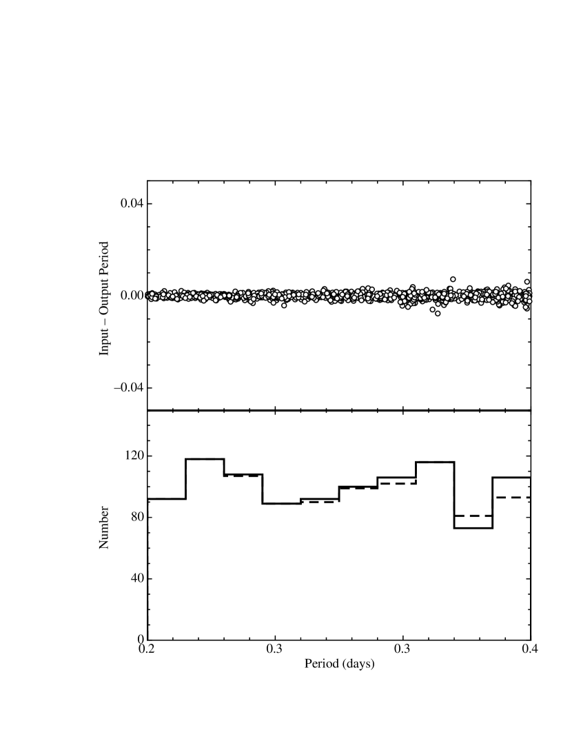
Figure 6: Same as Fig. 6 except that the simulations have been performed using an c-type RR Lyrae variable light curve.

Figure 7: The luminosity functions (LFs) for the non-variable stars in the two fields studied herein. The solid line in the lower panel is the F606W band LF for the field observed in 2005 (field 1 in Table 1) while the dashed line is the LF for the region observed in 2006 (field 2 in Table 1). The two upper panels show the variation of the photometric error as output by ALLFRAME with magnitude. We have plotted every 10th point to make the appearance of these plots manageable.

Figure 9: The upper panel shows the amplitude distribution of the c-type RR Lyraes from the present study (solid line) and the work of Brown et al. (2004, dotted line) scaled to the same maximum. The lower panel is the same as the upper one except that the ab-type RR Lyraes are plotted.

Figure 11: The period distributions of the ab-type (solid) and c-type (dotted) RR Lyrae variables. The dashed vertical lines represent the mean periods of these same stars from Brown et al. (2004). While the mean periods of the c-type variables agree between our study and that of Brown et al. (2004), the mean period of the ab-type RR Lyraes is somewhat shorter in our sample as compared with that of Brown et al.

Figure 12: The upper panel shows the metallicity distribution function for our sample of RRab variables using two different formulations for the conversion between period and metal abundance (solid line - Eqn (1), dashed line - Eqn (2)). The lower panel shows the MDFs derived using Eqn (2) for the two observed fields (dashed line - Field 2, solid line - Field 1).

References

- (1) Alcock, C. et al. 2000, AJ, 119, 2194
- (2) Alonso-García, J., Mateo, M., & Worthey, G. 2004, AJ, 127, 868
- (3) Brown, T. M. et al. 2004, AJ, 127, 2738 (B2004)
- (4) Castellani, M., Caputo, F., & Castellani, V. 2003, A&A, 410, 871
- (5) Chaboyer, B. 1999, in Post-Hipparcos cosmic candles, edited by A. Heck and F. Caputo. (Dordrecht ; Boston) Astrophysics and space science library, Vol. 237), p.111
- (6) Clement, C. M. 2000, in IAU COll. 176, The Impact of Large Scale Surveys on Pulsating Star Research, ed. L. Szabados & D. W. Kurtz (ASP Conf. Ser. 203) (San Francisco:ASP), 266
- (7) Clementini, G., Federici, L., Corsi, C., Cacciari, C., Bellazzini, M., & Smith, H. A. 2001, ApJ, 559, L109
- (8) Contreras, R., Federici, L., Clementini, G., Cacciari, C., Merighi, R., Kinemuchi, K., Catelan, M., Fusi Pecci, F., Marconi, M., Pritzl, B., & Smith, H. 2008, Memorie della Societa Astronomica Italiana, 79, 686
- (9) Dolphin, A. E., Saha, A., Olzsewski, E., Thim, F., Skillman, E. D., Gallagher, J. J., & Hoessel, J. 2004, AJ, 127, 875
- (10) Durrell, P. R., Harris, W. E., & Pritchet, C. J. 2001, AJ, 121, 2557
- (11) Freedman, W. L., & Madore, B. F. 1990, ApJ, 365, 186
- (12) Grebel, E. K., Gallagher, J. S. III, & Harbeck, D. 2003, AJ, 125, 1926
- (13) Grillmair, C. et al. 1996, AJ, 112, 1975
- (14) Guhathakurta, P. et al. 2005, arXiv preprint (astro-ph/0502366)
- (15) Horne, J. H. & Baliunas, S. L. 1986, ApJ, 302, 757
- (16) Irwin, M. J., Ferguson, A. M. N., Ibata, R. A., Lewis, G. F., & Tanvir, N. R. 2005, ApJ, 628, L108
- (17) Kalirai, J. S. et al. 2006, ApJ, 648, 389
- (18) Koch, A., & Grebel, E. K. 2006, 131, 1405
- (19) Koch, A., et al. 2008, ApJ, 689, 958
- (20) Layden, A. C. 1995, AJ, 110, 2312
- (21) Layden A. C., & Sarajedini, A. 2000, AJ, 119, 1760
- (22) Mack, J., Gilliland, R. L., Anderson. J., & Sirianni, M. 2007, ISR-ACS 2007-02
- (23) Mahmud, N. & Anderson, J. 2008, PASP,120, 907
- (24) Martin, N. F. et al. 2006, MNRAS, 371, 1983
- (25) Meylan, G. Sarajedini, A., Jablonka, P., Djorgovski, S. G., Bridges, T., & Rich, R. M. 2001, AJ, 122, 830
- (26) Mould, J., & Kristian, J. 1986, ApJ, 305, 591
- (27) Pritchet, C. J., & van den Bergh, S. 1987, ApJ, 316, 517
- (28) Reiss, A., & Mack, J. 2004, ISR-ACS 2004-06
- (29) Sandage, A. R. 1993, AJ, 106, 687
- (30) Sarajedini, A., Barker, M., Geisler, D., Harding, P., Schommer, R. 2006, AJ, 132, 1361
- (31) Sarajedini, A., & Jablonka, P. 2005, AJ, 130, 1627
- (32) Scargle, J. D. 1982, ApJ, 263, 835
- (33) Sirianni, M. et al. 2005, PASP, 117, 1049
- (34) Stetson, P. B. 1987, PASP, 99, 191
- (35) Stetson, P. B. 1994, PASP, 106, 250