Numerical Computation of First-Passage Times of Increasing Lévy Processes

Abstract

Let $\{D(s),\ s\geq 0\}$ be a non-decreasing Lévy process. The first-hitting time process $\{E(t)\ t\geq 0\}$ (which is sometimes referred to as an inverse subordinator) defined by $E(t)=\inf\{s:D(s)>t\}$ is a process which has arisen in many applications. Of particular interest is the mean first-hitting time $U(t)=\mathbb{E}E(t)$. This function characterizes all finite-dimensional distributions of the process $E$. The function $U$ can be calculated by inverting the Laplace transform of the function $\widetilde{U}(\lambda)=(\lambda\phi(\lambda))^{-1}$, where $\phi$ is the Lévy exponent of the subordinator $D$. In this paper, we give two methods for computing numerically the inverse of this Laplace transform. The first is based on the Bromwich integral and the second is based on the Post-Widder inversion formula. The software written to support this work is available from the authors and we illustrate its use at the end of the paper.

1 Introduction

Let $\{D(s),\ s\geq 0\}$ be a Lévy subordinator, that is, a non-decreasing Lévy process starting from $0$, which is continuous from the right with left limits. This process has stationary and independent increments and is characterized by its Laplace Transform

$$\mathbb{E}e^{-\lambda D(s)}=e^{-s\phi(\lambda)},\quad\lambda\geq 0.$$ (1)

The function $\phi$ above is known as the Lévy exponent (or Laplace exponent) and is given by the Lévy-Khintchine formula:

$$\phi(\lambda)=\mu\lambda+\int_{(0,\infty)}\left(1-e^{-\lambda x}\right)\Pi(dx),$$ (2)

where $\mu\geq 0$ is the drift and the Lévy measure $\Pi$ is a measure on $\mathbb{R}^{+}\cup\{0\}$ which satisfies $\int_{0}^{\infty}(1\wedge x)\Pi(dx)<\infty$ (see  [3],  [9] or  [10]).

Consider the inverse subordinator $\{E(t),\ t\geq 0\}$, which is given by the first-passage time of $D$:

$$E(t)=\inf\{s:D(s)>t\}.$$ (3)

The process $E(t)$ is non-decreasing, and its sample paths are a.s. continuous if and only if $D$ is strictly increasing. Also, $E$ is, in general, non-Markovian with non-stationary and non-independent increments.

Inverse subordinators are of particular interest in the study of fractional kinetics and the scaling limits of continuous time random walks, [7], [8], [20], [24],  [4]. Here, a Markov process, $\{X(t),t\geq 0\}$, is time-changed with an inverse subordinator, yielding the new process $M(t)=X(E(t))$, $t\geq 0$. For certain choices of subordinators $D$, using $E$ as a time change gives a model of anomalous diffusion, where the mean-squared displacement of $M$ grows non-linearly in time. For example, if $D$ is an $\alpha$-stable subordinator, that is, the subordinator whose Lévy exponent is given by

$$\phi(\lambda)=\lambda^{\alpha},\quad 0<\alpha<1,$$ (4)

then the mean of $E(t)$ is given by the power law $\mathbb{E}E(t)\sim t^{\alpha}$. Other types of non-linear behavior are also possible. In [20], Meerschaert considers the subordinator with Lévy exponent given by the following generalization of (4):

$$\phi(\lambda)=\int_{0}^{1}\lambda^{\beta}dp(\beta),$$ (5)

where $p$ is a probability measure on $(0,1)$. Depending on the choice of $p$, the mean of $E$ in this case can grow at logarithmic rates. Meerschaert also shows in this case that the transition density of the process $M$ solves a time-fractional diffusion equation whose order is distributed according to $p$.

Inverse Subordinators have also appeared in many other areas of probability theory. Early work regarding the joint distribution of $E(t)$ and $D(E(t))$ was done in [15] and [19]. More recently, in [18], Kaj and Martin-Löf show that a scaled sum of these processes converges weakly to another non-stable and non-Gaussian process. An application of inverse subordinators in modeling of foreign exchange markets was considered in [27]. Distributional properties of inverse subordinators were studied in [21], which drew upon a connection with Cox processes. A different approach using differential equations to characterize the joint distribution function of the process $E$ was used in [26] and [7].

An important function in the study of inverse subordinators is the so-called renewal function, $U(t)$, $t\geq 0$, which is given by the mean of the inverse subordinator, $U(t)=\mathbb{E}E(t)$. It has be shown by different methods that this function characterizes all finite-dimensional distributions of the process $E$. The Laplace transform of $U$ is given simply in terms of the Lévy exponent $\phi$, however, inverting this Laplace transform to obtain $U$ in closed form is not always possible. In this paper, we provide two numerical methods for obtaining this mean first-passage time which take as input the drift $\mu$ and the Lévy measure $\Pi$ of the corresponding subordinator $D$. Once $U$ is obtained, higher order moments can be calculated by methods described in [26] or [21].

This paper is organized as follows: We begin in Section 2 by giving a brief background on the theory of inverse subordinators, as well as describe the importance of the function $U$. In Section 3, we develop two methods for calculating $U$ numerically and test them in cases where $U$ can be computed analytically. In Section 4 we apply these techniques to the following examples: Poisson process with drift (Section 4.1), Compound Poisson process with Pareto jumps (Section 4.2), special cases of the “mixed” $\alpha$-stable process (Section 4.3), and the generalized inverse Gaussian Lévy process (Section 4.4). For each example, we compute one and two-time moments of $E$. Methods to compute $U$ for each example are implemented in MATLAB. The software for doing this is freely available from the authors and its use is described in Section 6.

2 Background

We start by recalling the fundamental relationship between a subordinator and its inverse. If $D$ is strictly increasing, then for $t_{1},t_{2},\dots,t_{n}$ and $s_{1},s_{2},\dots,s_{n}$ positive,

$$\{D(s_{i})<t_{i},i=1,\dots n\}=\{E(t_{i})>s_{i},i=1,\dots,n\}.$$ (6)

If $D$ is not strictly increasing, then the above relationship holds off a set of measure $0$ in $(t_{1},t_{2},\dots,t_{n})$ (see [26]).

As in the introduction, define the renewal function to be the mean of the inverse subordinator, $U(t)=\mathbb{E}E(t)$ for $t\geq 0$. Also, let $H_{s}(t)=P[D(s)<t]$. From the Lévy-Khintchine formula, we have $\int_{0}^{\infty}e^{-\lambda t}dH_{s}(t)=e^{-s\phi(\lambda)}$. This together with (6) lets us compute the Laplace transform, $\widetilde{U}$, of $U$:

$$\widetilde{U}(\lambda) = \int_{0}^{\infty}U(t)e^{-\lambda t}dt$$ (7)

$$= \int_{0}^{\infty}\int_{0}^{\infty}P[E(t)>s]e^{-\lambda t}dsdt$$ (8)

$$= \int_{0}^{\infty}\int_{0}^{\infty}P[D(s)<t]e^{-\lambda t}dsdt$$ (9)

$$= \int_{0}^{\infty}\int_{0}^{\infty}\frac{1}{\lambda}e^{-\lambda t}dH_{s}(t)ds$$ (10)

$$= \frac{1}{\lambda}\int_{0}^{\infty}e^{-s\phi(\lambda)}ds=\frac{1}{\lambda\phi(\lambda)}.$$ (11)

Thus, $\widetilde{U}$ characterizes the process $E$ (since $\phi$ characterizes $D$). Since $E$ is non-decreasing, we can define the Borel measure $dU$ which is induced by $U$, which is commonly referred to as the renewal measure. Notice that the renewal measure has the following property. For a.e. $0\leq a<b$, we have

$$\int_{0}^{\infty}\mbox{\boldmath$1$}_{(a,b]}(\tau)dU(\tau) = U(b)-U(a)$$ (12)

$$= \int_{0}^{\infty}P[E(b)>s]-P[E(a)>s]ds$$

$$= \int_{0}^{\infty}P[D(s)\leq b]-P[D(s)\leq a]ds$$

$$= \mathbb{E}\int_{0}^{\infty}\left(\mbox{\boldmath$1$}_{(-\infty,b]}(D(s))-\mbox{\boldmath$1$}_{(-\infty,a]}(D(s))\right)ds$$

$$= \mathbb{E}\int_{0}^{\infty}\mbox{\boldmath$1$}_{(a,b]}(D(s))ds.$$

By approximating with step functions, this relationship can be extended to continuous functions $g$ as $\int_{0}^{\infty}g(\tau)dU(\tau)=\mathbb{E}\int_{0}^{\infty}g(D(s))ds$. With this, we see the Laplace transform of $dU$ is given by

$$\int_{0}^{\infty}e^{-\tau\lambda}dU(\tau)=\mathbb{E}\int_{0}^{\infty}e^{-\lambda D(s)}ds=\int_{0}^{\infty}e^{-s\phi(\lambda)}ds=\frac{1}{\phi(\lambda)}.$$ (13)

The pair $U$ and $dU$ can be used to compute all joint moments of the process $E$. For non-negative integers $m_{1},\dots,m_{n}$ define

$$U(t_{1},\dots,t_{n};m_{1},\dots,m_{n})=\mathbb{E}E(t_{1})^{m_{1}}E(t_{2})^{m_{2}}\dots E(t_{n})^{m_{n}}.$$ (14)

The order of the moment in (14) is defined to be $N=\sum_{i=1}^{n}m_{i}$. The following theorem from [26] gives the $n$-time Laplace transform $\widetilde{U}(\lambda_{1},\dots,\lambda_{n};m_{1},\dots,m_{n})$ in terms of a strictly lower older moment.

Theorem 2.1

Let $D$ be a general Lévy subordinator with Lévy exponent $\phi$ and let $E$ be the inverse subordinator of $D$. The $n$-time Laplace Transform of the $N^{th}$ order moment $U(t_{1},\dots,t_{n};m_{1},\dots,m_{n})$ defined in (14) is given by

$$\widetilde{U}(\lambda_{1},\dots,\lambda_{n};m_{1},\dots,m_{n})=\frac{1}{\phi(\lambda_{1}+\dots+\lambda_{n})}\sum_{i=1}^{n}m_{i}\widetilde{U}(\lambda_{1},\dots,\lambda_{n};m_{1},\dots,m_{i-1},m_{i}-1,m_{i+1},\dots,m_{n}).$$ (15)

Notice that the Laplace transform of $U(t_{1},\dots,t_{n};m_{1},\dots,m_{n})$ is given as the product of $1/\phi$ and the Laplace transform of a strictly lower order moment. Taking inverse Laplace transforms, the $N^{th}$ order moment is given as the sum of convolutions

$$U(t_{1},\dots,t_{n};m_{1},\dots,m_{n})=\sum_{i=1}^{n}m_{i}\int_{0}^{\min_{i}t_{i}}U(t_{1}-\tau,\dots,t_{n}-\tau;m_{1},\dots,m_{i-1},m_{i}-1,m_{i+1},\dots,m_{n})dU(\tau).$$ (16)

For full details, see [26].

Thus, if one knows the function $U(t;1)=U(t)$, $t\geq 0$, then all higher order moments can be obtained inductively. For example, the covariance is given by

$$\mbox{Cov}(E(t_{1}),E(t_{2}))=\int_{0}^{t_{1}\wedge t_{2}}(U(t_{1}-\tau)+U(t_{2}-\tau))dU(\tau)-U(t_{1})U(t_{2}).$$ (17)

It is not always easy, however, to invert the Laplace transform (11) to obtain $U(t)$ analytically. In the following, we give two methods for numerically inverting this Laplace Transform given only the drift $\mu$ and Lévy measure $\Pi$ of the subordinator $D$. Once $U$ is obtained, the density of the renewal measure can be obtained by numerical differentiation and integral expressions such as (17) can be approximated by numerical integration. The first method is based on the Bromwhich integral which expresses the inverse Laplace transform as a path integral in the complex plane, and the second is based on the Post-Widder inversion formula, which expresses $U$ as a limit of terms involving derivatives of $\widetilde{U}$.

3 Computing $U(t)$

In Section 2 we saw that all moments of an inverse subordinator can be computed if one has first computed the renewal function $U(t)=\mathbb{E}E(t)$, which is given by the inverse Laplace transform of (11). In some cases, an analytical expression for $U$ can be found, and in most cases, the asymptotics of $U$ can be studied using a Tauberian Theorem. In this section we give two methods for calculating $U$ numerically. The first is simple and precise, but is difficult to use when $\phi$ is a complicated function. The second is more robust, but requires smoothness in $U$ to be effective.

3.1 Method 1: Numerical Integration

The first method involves calculating the inverse Laplace transform of $\widetilde{U}$ by numerically approximating the Bromwich integral:

$$U(t)=\frac{1}{2\pi i}\int_{b-i\infty}^{b+i\infty}e^{zt}\widetilde{U}(z)dz,$$ (18)

where $b$ is chosen such that $\widetilde{U}$ is analytic in the region $\mbox{Re}(z)\geq b$. Using the fact that $U(t)=0$ for $t<0$, and symmetry properties of analytic functions which are real valued on the real axis, (18) simplifies into two equivalent expressions:

$$U(t)=\frac{2e^{bt}}{\pi}\int_{0}^{\infty}\left(\mbox{Re}(\widetilde{U}(b+iu))\cos(ut)\right)du=\frac{-2e^{bt}}{\pi}\int_{0}^{\infty}\left(\mbox{Im}(\widetilde{U}(b+iu))\sin(ut)\right)du.$$ (19)

For details see [1].

From the Lévy Khintchine formula (2), we have

$$\phi(b+iu) = \mu b+i\mu u+\int_{0}^{\infty}\left(1-e^{-x(b+iu)}\right)\Pi(dx)$$ (20)

$$= \left(\mu b+\int_{0}^{\infty}\left(1-e^{-xb}\cos(xu)\right)\Pi(dx)\right)+i\left(\mu u-\int_{0}^{\infty}e^{-xb}\sin(xu)\Pi(dx)\right)$$ (21)

$$\equiv \phi_{r}(b+iu)+i\phi_{i}(b+iu).$$ (22)

Now, since $\widetilde{U}(\lambda)=(\lambda\phi(\lambda))^{-1}$, a simple calculation gives

$$\mbox{Re}(\widetilde{U}(b+iu)) = \frac{b\phi_{r}(b+iu)-u\phi_{i}(b+iu)}{(b^{2}+u^{2})(\phi_{r}(b+iu)^{2}+\phi_{i}(b+iu)^{2})}$$ (23)

$$\mbox{Im}(\widetilde{U}(b+iu)) = \frac{b\phi_{i}(b+iu)+u\phi_{r}(b+iu)}{(b^{2}+u^{2})(\phi_{r}(b+iu)^{2}+\phi_{i}(b+iu)^{2})}.$$ (24)

Since $\phi(0)=0$ and $\phi$ is increasing in $\lambda$, $\widetilde{U}(\lambda)=(\lambda\phi(\lambda))^{-1}$ has a singularity the origin. Therefore, we much choose $b>0$ above. Then, given $\mu$ and $\Pi$, we evaluate the integrals in (21) to obtain $\phi_{r}$ and $\phi_{i}$ and use (23) and (24) to obtain $\mbox{Re}(\widetilde{U}(b+iu))$ and $\mbox{Im}(\widetilde{U}(b+iu))$ for fixed $u$ and then compute either integral in (19) to get $U(t)$. Alternatively, if $\phi$ is known in closed form, then $\phi_{r}$ and $\phi_{i}$ can be computed directly. This method works fairly well when $\phi_{r}$ and $\phi_{i}$ are easy to compute, for instance, in the case of the Poisson process with drift. The main problem with the method is when the integrands in (19) and/or (21) are highly oscillatory and slowly decaying, causing most integration algorithms to converge very slowly.

3.2 Method 2: Post-Widder Inversion

The following method is based on the Post-Widder inversion formula ([1], Theorem 2 or  [12], section VII.6). In order to justify using this formula in our case, we state and prove this result under slightly weaker conditions than those found in  [12].

Theorem 3.1

(Post-Widder Inversion). Let $u:\mathbb{R}^{+}\rightarrow\mathbb{R}^{+}$ be a continuous function such that $u(x)/x\leq C$ as $x\rightarrow\infty$ for some $C\geq 0$, and let $\widetilde{u}(\lambda)$ be the Laplace transform of $u$. Then for $t>0$, we have

$$u(t)=\lim_{k\rightarrow\infty}\frac{(-1)^{k-1}}{(k-1)!}\left(\frac{k}{t}\right)^{k}\widetilde{u}^{(k-1)}\left(\frac{k}{t}\right),$$ (25)

where $\widetilde{u}^{(k)}$ denotes the $k^{th}$ derivative, $k\in\mathbb{Z}^{+}$.

Proof.

Fix $t>0$. Let $X_{i}$, $i=1,2,\dots$ be iid gamma random variables with mean $t$ and variance $t^{2}$ and let $M_{k}=\frac{1}{k}\sum_{i=1}^{k}X_{i}$. The idea is to approximate $u(t)$ by $\mathbb{E}u(M_{k})$. Notice that $M_{k}$ has a gamma distribution with mean $t$ and variance $t^{2}/k$. By the law of large numbers, $M_{k}\rightarrow^{d}t$ as $k\rightarrow\infty$ and by the continuous mapping theorem ([16], Theorem 5.10.4), $u(M_{k})\rightarrow^{d}u(t)$. Observe that we also have the following convergence in mean:

$$\mathbb{E}u(M_{k})\rightarrow u(t),$$ (26)

which follows from the uniform integrability of $u(M_{k})$. This can be seen using the density of a gamma random variable and the assumption that $u(x)\leq Cx$ as $x\rightarrow\infty$. Indeed, we have

$$\lim_{a\rightarrow\infty}\sup_{k\geq 1}\mathbb{E}u(M_{k})\mbox{\boldmath$1$}_{M_{k}>a} = \lim_{a\rightarrow\infty}\sup_{k\geq 1}\int_{a}^{\infty}u(x)x^{k-1}e^{-kx/t}dx$$ (27)

$$\leq \lim_{a\rightarrow\infty}\sup_{k\geq 1}C\int_{a}^{\infty}x^{k}e^{-kx/t}dx$$ (28)

$$= \lim_{a\rightarrow\infty}\sup_{k\geq 1}C\int_{a}^{\infty}(xe^{-x/t})^{k}dx$$ (29)

$$= \lim_{a\rightarrow\infty}C\int_{a}^{\infty}(xe^{-x/t})dx$$ (30)

$$= 0.$$ (31)

Now, (26) implies

$$u(t)=\lim_{k\rightarrow\infty}\mathbb{E}u(M_{k}) = \lim_{k\rightarrow\infty}\frac{1}{(k-1)!}\left(\frac{k}{t}\right)^{k}\int_{0}^{\infty}u(x)x^{k-1}e^{-kx/t}dx$$ (32)

$$= \lim_{k\rightarrow\infty}\frac{1}{(k-1)!}\left(\frac{k}{t}\right)^{k}\left((-1)^{k-1}\frac{\partial^{k-1}}{\partial\lambda^{k-1}}\int_{0}^{\infty}u(x)e^{-\lambda x}dx\right)\Big{|}_{\lambda=k/t}$$ (33)

$$= \lim_{k\rightarrow\infty}\frac{(-1)^{k-1}}{(k-1)!}\left(\frac{k}{t}\right)^{k}\widetilde{u}^{(k-1)}(k/t).$$ (34)

This verifies (25).  

• 1. In order to justify using the Post-Widder formula, we must be sure that the renewal function $U$ satisfies $U(t)/t\leq C$ as $t\rightarrow\infty$. Fortunately, the Renewal Theorem (see for instance, Proposition 3 in [21]) implies that if $D$ has finite mean, then $U(t)$ will grow as $O(t)$ as $t\rightarrow\infty$. If $D$ has infinite mean, its mean first hitting time $\mathbb{E}E(t)$ will, on average, grow slower than in the finite mean case for large $t$. To see this, any subordinator $D$ with infinite mean can be bounded below by a subordinator $\widehat{D}$ with finite mean by truncating the large jumps of $D$. The inverse, $\widehat{E}$, of $\widehat{D}$ will be a.s. greater than $E$, and thus $U(t)\leq\widehat{U}(t)=O(t)$.

2. One must check that $U$ is continuous before using the Post-Widder formula. Proposition A.1 in [26] implies that $U$ is continuous if $D$ is strictly increasing.

Thus, calculating $U(t)$ involves two steps:

1. Calculating

$$U_{k_{i}}(t)=\frac{(-1)^{k-1}}{(k_{i}-1)!}\left(\frac{k_{i}}{t}\right)^{k_{i}}\widetilde{U}^{(k_{i}-1)}\left(\frac{k_{i}}{t}\right)$$ (35)

for some set of integers $k_{1},k_{2},\dots,k_{n}$ (the choice of the $k_{i}$’s will be addressed later).

2. Using the values of $U_{k_{i}}(t)$, $i=1,\dots n$, to approximate the limit in (25).

We will first focus on step $1$ above. The main difficulty with using this method resides in the fact that (25) involves derivatives of arbitrarily high orders, which are often difficult to compute. Fortunately, in our case, this calculation can be done in a reasonable fashion, which we now outline. Recall Leibnitz’s formula, which states that for smooth functions $f,g$,

$$\frac{d^{k}}{dt^{k}}f(t)g(t)=\sum_{i=0}^{k}{k\choose i}g^{(k-i)}(t)f^{(i)}(t).$$ (36)

Let $k\geq 1$,$t>0$, and $\psi(\lambda)=1/\phi(\lambda)$. Applying Leibnitz’s formula to $\widetilde{U}(\lambda)=\lambda^{-1}\psi(\lambda)$ with $\lambda=k/t$ gives

$$\frac{(-1)^{k-1}}{(k-1)!}\left(\frac{k}{t}\right)^{k}\widetilde{U}^{(k-1)}(k/t) = \frac{(-1)^{k-1}}{(k-1)!}\left(\frac{k}{t}\right)^{k}\sum_{i=0}^{k-1}{k-1\choose i}\left(\frac{(-1)^{k-1-i}(k-1-i)!}{(k/t)^{k-i}}\right)\psi^{(i)}(k/t)$$ (37)

$$= \sum_{i=0}^{k-1}(-1)^{i}\frac{k^{i}}{i!t^{i}}\psi^{(i)}(k/t)$$ (38)

$$= \mbox{{v}}_{k}\cdot\mbox{{w}}_{k},$$ (39)

where the vectors $\textbf{v}_{k},\textbf{w}_{k}\in\mathbb{R}^{k}$ are given by

$$({\textbf{v}}_{k})_{i} = \left(\frac{(-1)^{i}k^{i}}{i!t^{i}}\right),\quad i=0,\dots,k-1$$ (40)

$$({\textbf{w}}_{k})_{i} = \left(\psi^{(i)}(k/t)\right),\quad i=0,\dots,k-1.$$ (41)

To compute the components of $\textbf{w}_{k}$, we use an idea from [22]. Using Leibnitz’s formula on the unit function $1=\phi(\lambda)\psi(\lambda)$, we see that for any $\lambda>0$,

$$\sum_{i=0}^{j}{j\choose i}\phi^{(j-i)}(\lambda)\psi^{(i)}(\lambda) = \frac{\partial^{j}}{\partial\lambda^{j}}\phi(\lambda)\psi(\lambda)$$ (42)

$$= \frac{\partial^{j}}{\partial\lambda^{j}}1$$ (43)

$$= \begin{cases}1\quad j=0,\\ 0\quad j\geq 1\end{cases},\quad j=0,\dots,k-1.$$ (44)

From this, we obtain the following matrix equation:

$$\left(\begin{array}[]{cccccc}\phi(\lambda)&0&0&0&\dots&0\\ \phi^{\prime}(\lambda)&\phi(\lambda)&0&0&\dots&0\\ \phi^{\prime\prime}(\lambda)&2\phi^{\prime}(\lambda)&\phi(\lambda)&0&\dots&0\\ \phi^{\prime\prime\prime}(\lambda)&3\phi^{\prime\prime}(\lambda)&3\phi^{\prime}(\lambda)&\phi(\lambda)&\dots&0\\ \vdots&&&&\ddots&\\ \phi^{(k-1)}(\lambda)&(k-1)\phi^{(k-2)}(\lambda)&&\dots&&\phi(\lambda)\end{array}\right)\left(\begin{array}[]{c}\psi(\lambda)\\ \psi^{\prime}(\lambda)\\ \psi^{\prime\prime}(\lambda)\\ \psi^{\prime\prime\prime}(\lambda)\\ \vdots\\ \psi^{(k-1)}(\lambda)\end{array}\right)=\left(\begin{array}[]{c}1\\ 0\\ 0\\ 0\\ \vdots\\ 0\end{array}\right).$$ (45)

Choosing $\lambda=k/t$, we conclude that $\textbf{w}_{k}$ satisfies the matrix equation $G_{k}\textbf{w}_{k}=e_{k}$, where $e_{k}=(1,0,\dots,0)^{\prime}\in\mathbb{R}^{k}$ and

$$(G_{k})_{ji}=\begin{cases}{j-1\choose i-1}\phi^{(j-i)}(k/t),\quad 1\leq i\leq j\leq k\\ 0,\quad\quad 1\leq j<i\leq k\end{cases}.$$ (46)

Observe that the entries in $G_{k}$ are easily expressed in terms of the drift $\mu$ and the Lévy measure $\Pi$ corresponding to the subordinator $D$. Indeed, we have

$$\phi^{(j)}(k/t)=\begin{cases}\displaystyle\mu\frac{k}{t}+\int_{0}^{\infty}\left(1-e^{-kx/t}\right)\Pi(dx),\quad j=0,\\ \\ \displaystyle\mu+\int_{0}^{\infty}xe^{-kx/t}\Pi(dx),\quad j=1,\\ \\ \displaystyle(-1)^{j+1}\int_{0}^{\infty}x^{j}e^{-kx/t}\Pi(dx),\quad j\geq 2\end{cases}.$$ (47)

Thus, to compute $\textbf{w}_{k}$, one needs to compute the entries of $G_{k}$ using (46) and (47), and then solve the matrix equation $G_{k}\textbf{w}_{k}=e_{k}$. Notice that the integrals in (47) are much easier to compute than those in Section 3.1 since the integrands do not oscillate; they decay exponentially and are positive. Observe that $\textbf{v}_{k}$, and hence $\textbf{v}_{k}\cdot\textbf{w}_{k}$ are easy to compute. Using this method, we get $U_{k_{i}}(t)=\textbf{v}_{k_{i}}\cdot\textbf{w}_{k_{i}}$ in (35).

• The density $U^{\prime}(t)$ of the renewal measure is also of interest, for example in (17). It can be approximated as $U$ is in (35), since the Laplace transform of $U^{\prime}(t)$ is $\psi(\lambda)$. One needs to compute $\psi^{(k-1)}(k/t)$, which is obtained with no extra cost from (45) since it is the last component of $\textbf{w}_{k}$.

For step 2 above, we refer to the technique explained in [13]. To summarize, it has been shown ([2],[17]) that if $U$ is smooth, then we have the following series expansion:

$$U_{k}(t)=U(t)+\sum_{m=1}^{\infty}\frac{a_{m}(t)}{k^{m}},$$ (48)

where $a_{m}(t)$ are remainder terms. Write $h_{i}=1/k_{i}$ and let $\widehat{U}_{h_{i}}(t)=U_{k_{i}}(t)$. With this, (48) implies

$$\widehat{U}_{h_{i}}(t)=U(t)+\sum_{m=1}^{\infty}a_{m}(t)h_{i}^{m}.$$ (49)

Our goal is to compute $\widehat{U}_{0}(t)=U(t)=\lim_{k\rightarrow\infty}U_{k}(t)$ with $t$ fixed. To do so, we consider $\widehat{U}_{h}(t)$ as a function of $h$ and, given $h_{1},h_{2},\dots,h_{n}$ and $\widehat{U}_{h_{1}},\dots,\widehat{U}_{h_{n}}$, we write down the so-called “Lagrange polynomial” $P_{n}(h)$: this is the polynomial of degree $n-1$ which passes through the $n$ points $(h_{i},\widehat{U}_{h_{i}}(t))$, $i=1,2,\dots,n$,

$$P_{n}(h)=\sum_{i=1}^{n}\left(\prod_{j\neq i}\frac{h-h_{j}}{h_{i}-h_{j}}\right)\widehat{U}_{h_{i}}(t).$$ (50)

Observe that if $h=h_{k}$ for some $k=1,2,\dots,n$, then all the summands in (50) vanish except for the term where $i=k$, which is equal to $\widehat{U}_{h_{k}}(t)$. Thus the polynomial $P_{n}(h)$ passes through the $n$ points $(h_{i},\widehat{U}_{h_{i}}(t))$, $i=1,2,\dots,n$.

Observe that we cannot compute $\widehat{U}_{0}(t)$ since $h=0$ corresponds to $k=\infty$. However, with the method described above, we can compute $\widehat{U}_{h_{i}}$ for $h_{i}\neq 0$ and then approximate $\widehat{U}_{0}(t)$ by $P_{n}(0)$. Since $\widehat{U}_{0}(t)=U(t)$, $U$ is then approximated by the linear combination

$$U(t)\approx P_{n}(0)=\sum_{i=1}^{n}c^{(n)}_{i}U_{k_{i}}(t),$$ (51)

where the weights $c^{(n)}_{i}$, calculated by setting $h=0$ in (50), depend on the choice of $\{h_{i}\}_{i=1}^{n}$.

Because the above method allows us to calculate $\widetilde{U}^{(k)}$ for large $k$, we shall take $k_{i}=2^{i-1}$, $i=1,2,\dots,n$. The corresponding weights $c_{i}^{(n)}$ are given by

$$c^{(n)}_{i}=\frac{(-1)^{n-i}2^{i(i-1)/2}}{\prod_{j=1}^{i-1}(2^{j}-1)\prod_{j=1}^{n-i}(2^{j}-1)},\quad i=1,2,\dots,n.$$ (52)

Thus, given a desired level of accuracy $\epsilon>0$ and $t>0$ fixed, we compute the sequence $P_{1}(0),P_{2}(0),\dots$ until $|P_{n}(0)-P_{n-1}(0)|<\epsilon$ and then set $U(t)=P_{n}(0)$. Typically this method converges with $n<9$ for reasonable values of $\epsilon$. Since $k_{10}=512$, it is often impossible to compute $U_{k_{i}}$ for $i\geq 10$ in double precision arithmetic, as noted in the remarks below.

Note that for (48) to hold and for this method to be most effective, $U$ must be sufficiently smooth. We found that for points at which $U$ is not differentiable, the sequence $P_{i}$ had a slower rate of convergence.

We close this section with two remarks regarding the computation of $U_{k}(t)$.

• Caution should be taken when computing terms like $k^{j}/j!$ for $k,j$ large, since numbers like $100^{100}$ and $200!$ are outside the range of double precision arithmetic. Instead, one should use expressions like $k^{j}/j!=\exp(j\log(k)-\sum_{i=1}^{j}\log(i))$, because while $k^{j}$ and $j!$ may be large, their ratio may be small. Nevertheless, for large enough $k$ and $j$ (relation (40), for example, which requires computing $k^{k-1}/(k-1)!$), even the ratio may be too large. This happens for instance if $k=k_{11}=2^{10}=1024$, in which case $1024^{1023}/1023!\approx 6.5\times 10^{442}$. To be safe, we used at most $k_{10}=512$.

• A similar overflow problem can occur for $k/t$ large. To avoid this, one can make the following adjustment to (25). Let $c>0$, then

  $$\frac{(-1)^{k-1}}{(k-1)!}\left(\frac{k}{t}\right)^{k}\widetilde{U}^{(k-1)}\left(\frac{k}{t}\right) = \frac{(-1)^{k-1}}{(k-1)!}\left(\frac{k}{ct}\right)^{k}c^{k}\widetilde{U}^{(k-1)}\left(\frac{k}{t}\right)$$ (53)

  $$= \frac{(-1)^{k-1}}{(k-1)!}\left(\frac{k}{ct}\right)^{k}\widetilde{U}^{(k-1)}\left(\frac{k}{ct};c\right),$$ (54)

  where $\widetilde{U}(\lambda;c)$ is a rescaled version of $\widetilde{U}$:

  $$\widetilde{U}(\lambda;c)\equiv c\widetilde{U}(c\lambda)=\frac{1}{\lambda\phi(c\lambda)}.$$ (55)

  Repeating the steps of this method with (54), we get

  $$U_{k}(t)=\widetilde{\textbf{v}}_{k}\cdot\widetilde{\textbf{w}}_{k},$$ (56)

  where $(\widetilde{\textbf{v}}_{k})_{i}=(\textbf{v}_{k})_{i}/c^{i}$ and $\widetilde{\textbf{w}}_{k}$ is the solution to the matrix equation $\widetilde{G}_{k}\widetilde{\textbf{w}}_{k}=e_{k}$, where $(\widetilde{G}_{k})_{ji}=(G_{k})_{ji}c^{j-i}$. To compute these products and ratios, a procedure as the one describes in the previous remark should be done to avoid overflow. We found the choice $c=t^{-1}$ useful.

3.3 Testing the methods

In Table 1, the Post-Widder method is tested in cases where $U$ can be computed explicitly (see Section 4 for explanations of each example). The values in the table were obtained using a threshold of $\epsilon=10^{-8}$. With the exception of starred entry in Table 1, all converged within this threshold with $n\leq 9$. If sufficient convergence did not occur, $P_{9}(t)$ is used as the approximation. In these cases, the approximation is very good.

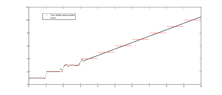
For the Poisson process, $U$ is discontinuous at the integers. Therefore, we used instead $t=1.1,10.1,100.1$. Since the Post-Widder method does not apply when $U$ is discontinuous, we do not expect to get good results in the Poisson case. And indeed, the absolute errors are large. For instance, Table 2 shows that when $t=10.1$, the algorithm converged but to the wrong value (the absolute error between the true and computed value is $0.4$). The plot in Figure 1 shows in more detail the erratic behavior of the Post-Widder method in this case. Notice that for larger times this method approximates $U$ (which in this case is a step function) with a straight line.

Subordinator	$t=0.01$	$t=0.1$	$t=1$	$t=10$	$t=100$
$\alpha$-stable ($\alpha=0.5$)	$2.5\times 10^{-13}$	$8.2\times 10^{-13}$	$1.7\times 10^{-13}$	$7.4\times 10^{-13}$	$2.6\times 10^{-11}$
Uniform Mixture of $\alpha$-stable	$7.8\times 10^{-12}$	$6.6\times 10^{-11}$	$1.4\times 10^{-10}$	$1.5\times 10^{-9}$	$8.7\times 10^{-10}$
Gamma Process ($\kappa=\gamma=1$)	$1.7\times 10^{-13}$	$7.0\times 10^{-14}$	$1.2\times 10^{-12}$	$3.4\times 10^{-10}$	$9.6\times 10^{-12}$
Inverse Gaussian($\gamma=\delta=1$)	$1.3\times 10^{-5*}$	$1.7\times 10^{-12}$	$1.3\times 10^{-11}$	$6.7\times 10^{-11}$	$3.0\times 10^{-9}$

Table 1: Absolute errors between exact values of $U$ and those given by this method for a selection of subordinators whose mean first passage time can be computed exactly. Here we used a threshold of $\epsilon=10^{-8}$.

In the cases where $U$ has little regularity, numerical integration (method 1) is the more accurate method. To see this, we applied the numerical integration method (using the MATLAB function quad) to the case of the Poisson process and obtained the absolute errors in Table 2. To compute these, we approximated the oscillatory integral in (19) by partitioning the range of integration $(0,\infty)$ into intervals of the form $I_{0}=(0,\pi/(2t)$, $I_{k}=[k\pi/(2t),(k+2)\pi/(2t)]$, $k\geq 1$, $k$ odd, and then summing the integrals over each $I_{k}$ until the contribution over one such interval became less then a threshold $\epsilon>0$. Due to the slowly decaying nature of the integrand, obtaining convergence for $\epsilon<10^{-6}$ is difficult.

We’ve found that integration is not feasible in many other cases (except possibly the $\alpha$-stable case).

Subordinator	$t=0.01$	$t=0.1$	$t=1.1$	$t=10.1$	$t=100.1$
Poisson Process (integration)	$1.08\times 10^{-6}$	$1.57\times 10^{-6}$	$3.6\times 10^{-11}$	$4.25\times 10^{-6}$	$1.09\times 10^{-4}$
Poisson Process (Post-Widder)	$<10^{-16}$	$7.1\times 10^{-10}$	$3.7\times 10^{-2*}$	$0.4$	$0.4$

Table 2: Absolute errors between exact values of $U$ and those given by numerical integration for the poisson process (whose mean first passage time can be computed exactly). Here we used a threshold of $\epsilon=10^{-6}$.

Figure 1: A comparison of the true value of $U$ for a Poisson process with no drift and its approximation given by the Post-Widder method. Since $U$ in this case has little regularity, the quality of the approximation is not always good.

4 Obtaining $U(t)=\mathbb{E}E(t)$ and $\mathrm{Corr}(E(s),E(t))$ for various inverse Lévy subordinators

We now present various examples of Lévy subordinators $\{D(s),s\geq 0\}$ and their inverses $\{E(t),t\geq 0\}$ and calculate the one time moment $U(t)=\mathbb{E}E(t)$ and the correlation function $\mathrm{corr}(E(s),E(t))$. We found the table of Laplace transforms [25] useful for some of the following calculations.

Since we will encounter Laplace transforms which cannot be inverted analytically, we will study their asymptotics using a Tauberian Theorem ([9] page 10), which we state here for convenience. Recall that a function $\ell(t)$, $t>0$, is slowly varying at $0$ (respectively $\infty$) if for all $c>0$, $\lim(\ell(ct)/\ell(t))=1$ as $t\rightarrow 0$ (respectively $t\rightarrow\infty$).

Theorem 4.1

(Tauberian Theorem) Let $\ell:(0,\infty)\rightarrow(0,\infty)$ be a slowly varying function at $0$ (respectively $\infty$) and let $\rho\geq 0$. Then for a function $U:(0,\infty)\rightarrow(0,\infty)$, the following are equivalent:

(i) $U(x)\sim x^{\rho}\ell(x)/\Gamma(1+\rho),\quad x\rightarrow 0$ (respectively $x\rightarrow\infty$).

(ii) $\widetilde{U}(\lambda)\sim\lambda^{-\rho-1}\ell(1/\lambda),\quad\lambda\rightarrow\infty$ (respectively $\lambda\rightarrow 0$).

4.1 Poisson process

Consider the process $D(s)=\mu s+N(s)$, where $\{N(s),s\geq 0\}$ is a Poisson process with rate $r>0$. The Lévy exponent for this is given by

$$\phi(\lambda)=\mu\lambda+r(1-e^{-\lambda}),$$ (57)

and the Lévy measure $\Pi(dx)$ is a point-mass at $x=1$ with weight $r$. The sample paths of $D$ are straight lines with slope $\mu$, together with jumps of size $1$ which happen at random times $\{\tau_{k}\}_{k=1}^{\infty}$, such that $\{\tau_{i}-\tau_{i-1}\}_{i=1}^{\infty}$ are iid exponential with mean $1/r$.

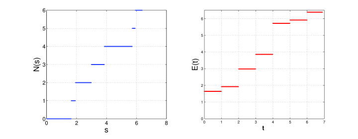
First consider the case with no drift, $\mu=0$. Figure 2 displays a sample path of the Poisson process $N(s)$ together with its inverse $E(t)$ which is the first time $N(s)$ exceeds the level $t$. Notice that each segment in the plot of $E$ has length $1$. For any $0<t_{0}<1$, one must wait a random time $\tau_{1}$ for the process $N$ to surpass $t_{0}$, thus $E(t_{0})=\tau_{1}$. More generally, the inverse subordinator $E(t)$ is a sum of $\lfloor t+1\rfloor$ iid exponential random variables with mean $1/r$, implying $E(t)\sim\Gamma(\lfloor t+1\rfloor,1/r)$.

Figure 2: A sample path of the Poisson process $N(s)$ together with its inverse.

Using the density of a Gamma random variable, the $\gamma$-moment of the $E(t)$, with $\gamma>0$, is given by

$$\mathbb{E}E(t)^{\gamma} = \frac{r^{\lfloor t+1\rfloor}}{\Gamma(\lfloor t+1\rfloor)}\int_{0}^{\infty}x^{\gamma}x^{\lfloor t+1\rfloor-1}e^{-xr}dx$$ (58)

$$= \frac{r^{\lfloor t+1\rfloor}\Gamma(\lfloor t+1\rfloor+\gamma)}{\Gamma(\lfloor t+1\rfloor)r^{\lfloor t+1\rfloor+\gamma}}$$ (59)

$$= \frac{\Gamma(\lfloor t+1\rfloor+\gamma)}{r^{\gamma}\Gamma(\lfloor t+1\rfloor)}.$$ (60)

Setting $\gamma=1$ yields $U(t)=\lfloor t+1\rfloor/r$ and the renewal measure, $dU(t)$, for the Poisson process is the measure which assigns a mass of $1/r$ to each integer $n\geq 0$. The covariance, (17), of this process is then given by

$$\mbox{\rm Cov}(E(s),E(t))=\left(\sum_{k=0}^{\lfloor s\wedge t\rfloor}\frac{U(s-k)}{r}+\frac{U(t-k)}{r}\right)-U(s)U(t).$$ (61)

Now assume positive drift, i.e. $\mu>0$. From (11) and (57), the Laplace transform of $U(t)$ is given by

$$\widetilde{U}(\lambda)=\frac{1}{\lambda(\mu\lambda+r(1-e^{-\lambda}))}.$$ (62)

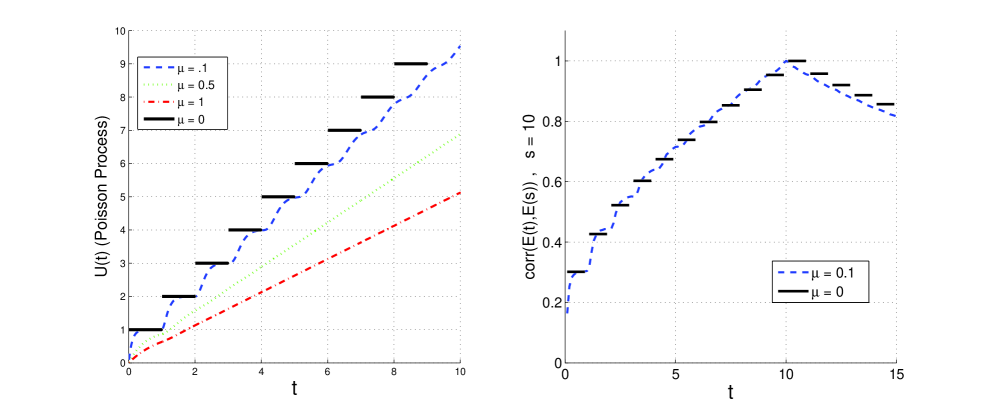
Due to the simple form of $\widetilde{U}(t)$, $U(t)$ can be calculated by numerical integration (i.e. method 1 in Section 3) . In Figure 3 we plot $U(t)=\mathbb{E}E(t)$ for various values of $\mu$, namely $\mu=0,0.1,0.5,1$. We also compute the correlation coefficient. It is obtained using (61) in the case of no drift but it is not known in closed for $\mu>0$. To compute for $\mu>0$, we use (17). The integral in (17) involves the renewal measure $dU$, but since in this case the function $U(t)$ is strictly increasing and continuous for $\mu$ positive, $dU$ is given by $U^{\prime}(t)dt$. We obtain $U^{\prime}(t)$ here by discrete approximation. The correlation coefficient $\mbox{corr}(E(s),E(t))$ is plotted in Figure 3 as a function of $t$ with $s=10$ fixed for zero and non-zero drift.

Figure 3: (Left) Plots of $\mathbb{E}E(t)$, where $E$ is the inverse of a Poisson process with rate $r=1$ and various drifts. For $\mu>0$, these plot were generated using the numerical integration method in Section 3.1. (Right) The correlation coefficient $\mbox{corr}(E(s),E(t))$ of the Poisson process with $s=10$ fixed and $t$ varying with drifts $\mu=0$ and $\mu=0.1$. This was calculated using (61) in the case $\mu=0$ and by numerical approximation of the integral in equation (17) for $\mu>0$. Since here $s=10$, the correlation equals $1$ when $t=10$ as well.

4.2 Compound Poisson processes

Let $\xi_{i}$ $i=1\dots$ be positive iid random variables with probability measure $\nu$. The compound Poisson process, $X(s)$, $s\geq 0$ is defined by

$$D(s)=\sum_{k=1}^{N(s)}\xi_{i},$$ (63)

where $N(s)$ is a Poisson process with rate $1$. In this case, the Lévy measure $\Pi$ in (2) is given by the distribution of the random variable $\xi_{1}$. Therefore, the Lévy exponent for this process is

$$\phi(\lambda)=\int_{0}^{\infty}(1-e^{-\lambda x})\nu(dx).$$ (64)

Notice that $X(t)=0$ for all $t<\tau_{1}$, where $\tau_{1}$ has an exponential distribution with mean $1$. This implies that $E(0)$ will also have an exponential distribution, and thus $E(0)\neq 0$ a.s. The fact that $E(0)\neq 0$ is characteristic of compound Poisson processes. Indeed, suppose that the inverse of a subordinator $D$ satisfies $E(0)>0$ a.s., then in particular, $\mathbb{E}E(t)\rightarrow c>0$ at $t\rightarrow 0$ since $E$ has cadlag paths. Thus, by the Tauberian Theorem,

$$\widetilde{U}(\lambda)=\frac{1}{\lambda\phi(\lambda)}\sim{\cal{L}}[c](\lambda)=\frac{c}{\lambda},\quad\lambda\rightarrow\infty.$$ (65)

Thus, $\phi(\lambda)/c\rightarrow 1$ as $\lambda\rightarrow\infty$, implying $\phi$ is bounded, which means $D$ is a Compound Poisson process (see [9], Corollary I.1.3).

Now focus on the special case when $\xi_{1}$ has a Pareto distribution, meaning $\xi_{1}$ has probability density $\nu(x)=\alpha x^{-\alpha-1}$ for $x\geq 1$, and $\alpha>0$ is fixed. The Lévy exponent is given by

$$\phi(\lambda)=\alpha\int_{1}^{\infty}(1-e^{-\lambda x})x^{-\alpha-1}dx=1-\alpha\mbox{ \rm Ei}_{1+\alpha}(\lambda),$$ (66)

where $\mbox{ \rm Ei}_{\alpha+1}(\lambda)=\int_{1}^{\infty}\frac{e^{-\lambda x}}{x^{\alpha+1}}dx$ is the Exponential integral. Using a series expansion of $\mbox{ \rm Ei}_{\alpha+1}$, we have

$$\phi(\lambda)\sim\begin{cases}-\alpha\Gamma(-\alpha)\lambda^{\alpha}\quad 0<\alpha<1\\ (1-\gamma_{e}-\log(\lambda))\lambda\quad\alpha=1\\ \frac{\alpha}{\alpha-1}\lambda\quad\alpha>1\end{cases}\quad\lambda\rightarrow 0,$$ (67)

where $\gamma_{e}\approx 0.5772$ is the Euler constant. Since $\widetilde{U}(\lambda)=(\lambda\phi(\lambda))^{-1}$, the Tauberian Theorem gives the large time behavior of the first passage time for this Compound Poisson process

$$U(t)\sim\begin{cases}\displaystyle\frac{1}{-\alpha\Gamma(-\alpha)\Gamma(1+\alpha)}t^{\alpha},\quad 0<\alpha<1\\ \\ \displaystyle\frac{1}{1-\gamma_{e}+\log(t)}t\quad\alpha=1\\ \\ \displaystyle\frac{\alpha-1}{\alpha}t,\quad\alpha>1\end{cases},\quad t\rightarrow\infty.$$ (68)

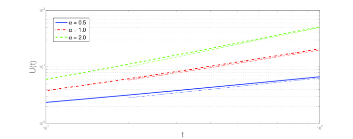
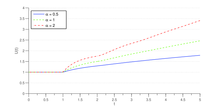
To calculate $U$, we found the Post-Widder method in Section 3 to be most useful. In Figure 4 we plot $U$ for $\alpha=1/2,1,2$, and in Figure 5 we plot $U$ along with the asymptotic expressions given in (68) with log-log scale. The correlation $\mathrm{corr}(E(t),E(s))$ is plotted in Figure 6. Note that the renewal measure $dU$ will give a mass of weight $1$ to $t=0$ since $U$ has a jump of size $1$ there. For $t>0$, $dU$ is a measure which has density $U^{\prime}(t)$ which can be calculated as $U$ is with the Post-Widder method as noted in a remark in Section 3.2.

Figure 4: The mean first passage time of the compound Poisson process with Pareto jumps computed using the Post-Widder inversion method for $\alpha=0.5,1,2$.

Figure 5: A log-log plot of the mean first passage time of the compound Poisson process with Pareto jumps computed using the Post-Widder inversion method for $\alpha=0.5,1,2$. The dotted lines represent the asymptotic expressions given in (68). We see good agreement for large times.

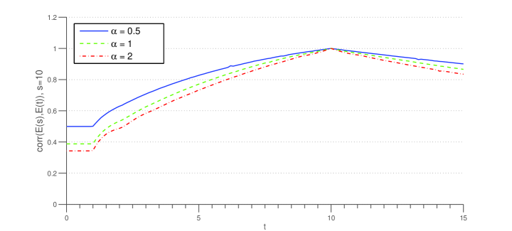
Figure 6: The correlation coefficient $\mbox{corr}(E(t),E(s))$ with $s=10$ fixed for the compound process with Pareto jumps for $\alpha=0.5,1,2$.

4.3 “Mixture” of $\alpha$-stable subordinators

We consider here a continuous mixture of $\alpha$-stable subordinators with $0<\alpha<1$. Namely, the subordinator whose Lévy exponent is given by

$$\phi(\lambda) = \int_{0}^{1}p(\beta)\lambda^{\beta}d\beta$$ (69)

$$= \int_{0}^{\infty}(1-e^{-\lambda x})g_{p}(x)dx,$$ (70)

where $p$ is a probability density on $(0,1)$ and the density $g_{p}$ of the Lévy measure is given by

$$g_{p}(x)=\int_{0}^{1}\frac{x^{-\beta-1}}{\Gamma(-\beta)}p(\beta)d\beta$$ (71)

In general, this subordinator has no finite moments. The $\alpha$-stable subordinator corresponds to the choice $p(\beta;\alpha)=\delta(\beta-\alpha)$ in (69). Here we will consider two extensions of this, namely when we choose a sum of two $\alpha$-stables, $p(\beta;\alpha_{1},\alpha_{2})=C_{1}\delta(\beta-\alpha_{1})+C_{2}\delta(\beta-\alpha_{2})$, with $\alpha_{2}<\alpha_{1}$ and $C_{1}+C_{2}=1$, as well as what we call the “uniform mix”, which corresponds to the choice $p(\beta)=1$ on $(0,1)$.

4.3.1 Single $\alpha$-stable

Many properties of the inverse of an $\alpha$-stable subordinator with $0<\alpha<1$ are known (see for instance, [7]), but we restate them here for convenience. Consider the $\alpha$-stable subordinator $\{D_{\alpha}(s),\ s\geq 0\}$ with Lévy exponent $\phi(\lambda)=\lambda^{\alpha}$. Taking the inverse Laplace transform of (11), we have that the mean first passage time for an inverse $\alpha$-stable subordinator is given by

$$U(t)=\frac{t^{\alpha}}{\Gamma(1+\alpha)},$$ (72)

which implies that the density of the renewal measure is $U^{\prime}(t)=t^{\alpha-1}/\Gamma(\alpha)$. With this, the covariance can be given in closed form. Assume $s\leq t$, then

$$\mbox{\rm Cov}(E(s),E(t)) = \frac{1}{\Gamma(1+\alpha)\Gamma(\alpha)}\int_{0}^{s}\left((t-\tau)^{\alpha}+(s-\tau)^{\alpha}\right)\tau^{\alpha-1}d\tau-\frac{(st)^{\alpha}}{\Gamma(1+\alpha)^{2}}$$ (73)

$$= \frac{s^{2\alpha}}{\Gamma(1+2\alpha)}+s^{\alpha}t^{\alpha}\left(\frac{1}{\Gamma(1+\alpha)}F(\alpha,-\alpha,\alpha+1;s/t)-\frac{1}{\Gamma(1+\alpha)^{2}}\right).$$ (74)

The above integral was computed in Mathematica and $F$ denotes the regularized confluent hypergeometric function.

4.3.2 Sum of two $\alpha$-stable subordinators

Here we consider the case when $p(\beta)=C_{1}\delta(\beta-\alpha_{1})+C_{2}\delta(\beta-\alpha_{2})$ and the Lévy exponent is given by

$$\phi(\lambda)=C_{1}\lambda^{\alpha_{1}}+C_{2}\lambda^{\alpha_{2}},$$ (75)

where $\alpha_{2}<\alpha_{1}$ and $C_{1}+C_{2}=1$. This corresponds to the subordinator given by $C_{1}^{1/\alpha_{1}}D_{\alpha_{1}}(s)+C_{2}^{1/\alpha_{2}}D_{\alpha_{2}}(s)$. From (11), the Laplace transform of the mean first passage time is given by

$$\widetilde{U}(\lambda)=\frac{1}{C_{1}\lambda^{\alpha_{1}+1}+C_{2}\lambda^{\alpha_{2}+1}}.$$ (76)

Using the Tauberian Theorem, $U$ has the following behavior in the limits $t\rightarrow 0$ and $t\rightarrow\infty$,

$$U(t)\sim\begin{cases}\displaystyle\frac{t^{\alpha_{1}}}{C_{1}\Gamma(1+\alpha_{1})},\quad t\rightarrow 0\\ \\ \displaystyle\frac{t^{\alpha_{2}}}{C_{2}\Gamma(1+\alpha_{2})},\quad t\rightarrow\infty.\end{cases}$$ (77)

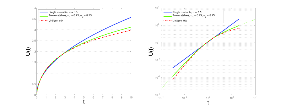
Thus, we see a cross-over in power-law behavior (which is displayed with a log-log plot in Figure 7). A closed form for the inverse Laplace transform of (76) could not be found, however $U$ can be calculated numerically using the Post-Widder method (method 2 in Section 3). Figure 7 shows plots of this function for various parameter values.

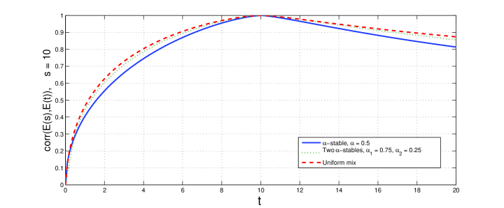
To obtain the correlation, we set $dU(t)=U^{\prime}(t)dt$, calculated $U^{\prime}(t)$ using the Post-Widder method and then evaluated the integrand in (17) using numerical integration. The correlation is plotted in Figure 8.

Figure 7: Plot of $U(t)$ calculated with the Post-Widder method for a single $\alpha$-stable, a sum of two $\alpha$ stables, and a uniform mixture. On the right we used a log-log plot and dotted lines to show asymptotic behavior given by (77) for the sum of two $\alpha$-stable case.

4.3.3 Uniform mixture

Here we consider the case when $p(\beta)=1$, for $\beta\in(0,1)$. The Lévy exponent is given by

$$\phi(\lambda)=\int_{0}^{1}\lambda^{\beta}d\beta=\frac{\lambda-1}{\log(\lambda)}.$$ (78)

The mean-first passage time for the inverse of this process has a closed form expression given by (see [25], Eq. 4.1.9)

$$U(t)={\cal L}^{-1}\frac{1}{\lambda\phi(\lambda)}={\cal{L}}^{-1}\frac{\log(\lambda)}{\lambda^{2}-\lambda}=\gamma_{e}+e^{t}\Gamma(0,t)+\log(t).$$ (79)

Here $\Gamma(0,t)$ is the incomplete gamma function given by $\Gamma(0,t)=\int_{t}^{\infty}e^{-z}z^{-1}dz$. Since, for $t$ large,

$$e^{t}\Gamma(0,t)=\int_{t}^{\infty}e^{-(z-t)}z^{-1}dz\leq\int_{0}^{\infty}e^{-z}dz=1,$$ (80)

we obtain the “ultraslow” growth:

$$U(t)\sim\log(t),\quad t\rightarrow\infty.$$ (81)

The density of the renewal measure also has a nice form:

$$U^{\prime}(t)=e^{t}\Gamma(0,t)-e^{t}e^{-t}t^{-1}+t^{-1}=e^{t}\Gamma(0,t).$$ (82)

Using this, we can numerically calculate the covariance for the inverse of the uniform mixed subordinator with (17). The correlation is plotted in Figure 8.

Figure 8: A plot of the correlation coefficient with $s$ fixed at $10$ and $t$ varying for the $\alpha$-stable process with $\alpha=1/2$, the sum of two $\alpha$-stables with $\alpha_{1}=.75$ and $\alpha_{2}=.25$ and the uniform mix. The correlation for the $\alpha$-stable case can be calculated exactly using (74). In the other two cases, we numerically approximated the integral in (17).

4.4 Generalized inverse Gaussian Lévy processes

The generalized inverse Gaussian (GIG) distribution [6], [11] is a distribution characterized by three parameters $\delta,\gamma,\kappa$ and has probability density function given by

$$p_{GIG(\delta,\gamma,\kappa)}(x)=\left(\frac{\gamma}{\delta}\right)^{\kappa}\frac{1}{2K_{\kappa}(\delta\gamma)}x^{\kappa-1}e^{-\frac{1}{2}(\delta^{2}x^{-1}+\gamma^{2}x)},\quad x>0.$$ (83)

Here, $K_{\kappa}$ denotes the modified Bessel function of the third kind ([14], section 3.2). The parameters of this distribution may take the following values:

$$\delta\geq 0,\ \gamma>0, \ \kappa>0,$$ if (84)

$$\delta>0,\ \gamma>0, \ \kappa=0,$$ if (85)

$$\delta>0,\ \gamma\geq 0, \ \kappa<0.$$ if (86)

Important subclasses in this family are

• $\kappa>0$, $\delta=0$, $\gamma>0$ gives a Gamma distribution $\Gamma(\kappa,2/\gamma^{2})$ with density

  $$p_{GIG(0,\gamma,\kappa)}(x)=\frac{\gamma^{2\kappa}}{2^{\kappa}\Gamma(\kappa)}x^{\kappa-1}e^{-\frac{\gamma^{2}}{2}x},\quad x>0,\kappa>0,\gamma>0.$$ (87)

• $\kappa<0$, $\delta>0$, $\gamma=0$ gives a reciprocal Gamma distribution $\mathrm{R}\Gamma(\kappa,\delta^{2}/2)$ with density

  $$p_{GIG(\delta,0,\kappa)}(x)=\frac{\delta^{-2\kappa}}{2^{-\kappa}\Gamma(-\kappa)}x^{\kappa-1}e^{-\frac{\delta^{2}}{2x}},\quad x>0,\kappa<0,\delta>0.$$ (88)

  This distribution only has finite moments of order less than $|\kappa|$.

• $\kappa=-\frac{1}{2}$, $\delta>0$,$\gamma\geq 0$ gives an Inverse Gaussian distribution $\mathrm{IG}(\delta,\gamma)$ with density

  $$p_{GIG(\delta,\gamma,-1/2)}(x)=\frac{\delta e^{\gamma\delta}}{\sqrt{2\pi}}x^{-3/2}e^{-\frac{1}{2}(\delta^{2}x^{-1}+\gamma^{2}x)},\quad x>0,\gamma\geq 0,\delta>0.$$ (89)

  The Inverse Gaussian distribution is the distribution of the first time a Brownian motion with variance $\delta$ and drift $\gamma$ reaches the level $1$ ([3], Example 1.3.21). All moments are finite if $\gamma>0$, but if $\gamma=0$, it becomes a totally right-skewed $\frac{1}{2}$-stable distribution which only has finite moments of order less than $1/2$.

The GIG distribution was shown to be infinitely divisible in [5] and its Lévy-Khintchine representation was derived in Section 5 of [11]. The Lévy-Khintchine representation given in [11] is not in the form (2) and some computation is needed to bring it into this form. This is done in appendix A.

The Laplace transform of $p_{GIG(\delta,\gamma,\kappa)}$ for $\delta>0$ and $\gamma>0$ is given by

$$\widetilde{p}_{GIG(\delta,\gamma,\kappa)}(\lambda) = \left(\frac{\gamma^{2}}{\gamma^{2}+2\lambda}\right)^{\kappa/2}\frac{K_{\kappa}(\delta\sqrt{\gamma^{2}+2\lambda})}{K_{\kappa}(\delta\gamma)}$$ (90)

$$= \exp(-\phi_{GIG(\delta,\gamma,\kappa)}(\lambda)),$$ (91)

where the Lévy exponent $\phi_{GIG}$ is given by

$$\phi_{GIG(\delta,\gamma,\kappa)}(\lambda)=\int_{0}^{\infty}(1-e^{-\lambda x})g_{GIG(\delta,\gamma,\kappa)}(x)dx,$$ (92)

Thus, the Lévy exponent is of the form (2) with drift $\mu=0$. The corresponding Lévy measure (density) is (see [11] or Appendix A)

$$g_{GIG(\delta,\gamma,\kappa)}(x)=\frac{e^{-\frac{\gamma^{2}}{2}x}}{x}\left(\int_{0}^{\infty}\frac{e^{-xy}}{\pi^{2}y(J^{2}_{|\kappa|}(\delta\sqrt{2y})+Y^{2}_{|\kappa|}(\delta\sqrt{2y}))}dy+\max(0,\kappa)\right),\quad x>0.$$ (93)

Here, $J_{\nu}$ and $Y_{\nu}$ denote the Bessel function of the first and second kind, respectively, with index $\nu$ ([14], Chapter 2).

By letting $\delta\rightarrow 0$ with $\kappa>0$ and $\gamma\rightarrow 0$ with $\kappa<0$ in (90), we obtain the Laplace transform of the gamma distribution (87) and the reciprocal gamma distribution (88) respectively. Doing so gives (see [11])

$$\widetilde{p}_{GIG(0,\gamma,\kappa)}(\lambda) = \left(1+\frac{2\lambda}{\gamma^{2}}\right)^{-\kappa}\quad\kappa,\gamma>0,$$ (94)

$$\widetilde{p}_{GIG(\delta,0,\kappa)}(\lambda) = \frac{2\left(\frac{\delta^{2}}{2}\right)^{-\kappa/2}\lambda^{-\kappa/2}}{\Gamma(-\kappa)}K_{-\kappa}(\delta\sqrt{2\lambda}),\quad\kappa<0,\delta>0.$$ (95)

The corresponding Lévy measures are obtained similarly using (93), (recall that $Y_{\nu}(z)\rightarrow-\infty$ as $z\rightarrow 0$):

$$g_{GIG(0,\gamma,\kappa)}(x) = \frac{\kappa}{x}e^{-\frac{\gamma^{2}}{2}x}$$ (96)

$$g_{GIG(\delta,0,\kappa)}(x) = \frac{1}{x}\int_{0}^{\infty}\frac{e^{-xy}}{\pi^{2}y(J^{2}_{|\kappa|}(\delta\sqrt{2y})+Y^{2}_{|\kappa|}(\delta\sqrt{2y}))}dy.$$ (97)

The mean of a GIG distribution, when it exists, can be calculated from these Laplace transforms. If $X\sim GIG(\delta,\gamma,\kappa)$, then there are three cases for $\mathbb{E}X$:

$$\mathbb{E}X = \frac{\delta K_{1+\kappa}(\gamma\delta)}{\gamma K_{\kappa}(\gamma\delta)},\quad\kappa\in\mathbb{R},\gamma>0,\delta>0$$ (98)

$$\mathbb{E}X = \frac{2\kappa}{\gamma^{2}},\quad\delta=0,\kappa>0,\gamma>0$$ (99)

$$\mathbb{E}X = \begin{cases}\infty,\quad\gamma=0,\quad-1\leq\kappa<0,\delta>0\\ \frac{1}{2(-\kappa-1)}\delta^{2},\quad\quad\quad\gamma=0,\kappa<-1,\delta>0\end{cases}$$ (100)

We talked so far about the GIG distribution. We now consider the corresponding Lévy process, namely, the subordinator $\{D_{GIG(\delta,\gamma,\kappa)}(s),\ s\geq 0\}$ with Laplace transform

$$\mathbb{E}\exp(-\lambda D_{GIG(\delta,\gamma,\kappa)}(s))=\exp(-s\phi_{GIG(\delta,\gamma,\kappa)}(\lambda)).$$ (101)

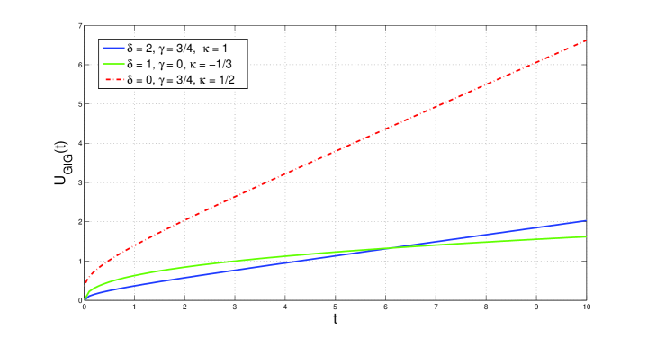
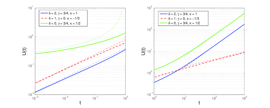
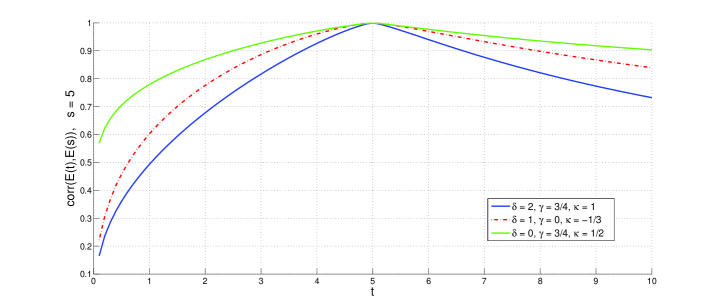
From (92), the drift of this process is $0$ and its Lévy measure is given by $\Pi(dx)=g_{GIG}(x)dx$. Notice that this Lévy process is indeed a subordinator since its Lévy measure is concentrated on the positive axis and from (96) and (97), it follows that $\int_{0}^{\infty}(1\wedge x)\Pi(dx)<\infty$. Let $E_{GIG(\delta,\gamma,\kappa)}$ be the inverse of $D_{GIG(\delta,\gamma,\kappa)}$ and let $U_{GIG(\delta,\gamma,\kappa)}(t)=\mathbb{E}E_{GIG(\delta,\gamma,\kappa)}(t)$. The gamma process ($\delta=0$) and the inverse Gaussian process ($\kappa=-1/2$) are treated in [21], where closed form expressions are given for the renewal measure. In general, we cannot write $U_{GIG}(t)$ in closed form, however, we can obtain expressions for large and small time behavior using the Tauberian theorem.

Asymptotics of $U_{GIG(\delta,\gamma,\kappa)}$, $t\rightarrow 0$: One has $K_{\kappa}(x)\sim\sqrt{\frac{\pi}{2x}}e^{-x}$ as $x\rightarrow\infty$ ( [14], section 5.4). We first consider the case when $\delta>0$. When $\gamma>0$, (90) implies that as $\lambda\rightarrow\infty$,

$$\phi_{GIG(\delta,\gamma,\kappa)}(\lambda) = -\log\left(\left(\frac{\gamma^{2}}{\gamma^{2}+2\lambda}\right)^{\kappa/2}\frac{K_{\kappa}(\delta\sqrt{\gamma^{2}+2\lambda})}{K_{\kappa}(\delta\gamma)}\right)$$ (102)

$$= \frac{\kappa}{2}\log\left(1+\frac{2\lambda}{\gamma^{2}}\right)-\log(K_{k}(\delta\sqrt{\gamma^{2}+2\lambda}))+\log(K_{\kappa}(\delta\gamma))$$ (103)

$$= \delta\sqrt{\gamma^{2}+2\lambda}+O(\log(\lambda))$$ (104)

$$\sim \delta\sqrt{2\lambda},\quad\lambda\rightarrow\infty.$$ (105)

The case $\gamma=0$ gives the same answer (by using (95)). If $\delta=0$, we instead use (94) and get

$$\phi_{GIG(0,\gamma,\kappa)}(\lambda) = \kappa\log\left(1+\frac{2\lambda}{\gamma^{2}}\right)$$ (106)

$$\sim \kappa\log(\lambda),\quad\lambda\rightarrow\infty.$$ (107)

Since $\widetilde{U}_{GIG(\delta,\gamma,\kappa)}(\lambda)=(\lambda\phi_{GIG(0,\gamma,\kappa)}(\lambda))^{-1}$, we get from the Tauberian theorem

$$U_{GIG(\delta,\gamma,\kappa)}(t)\sim\begin{cases}\displaystyle\frac{-1}{\kappa\log(t)},\quad\delta=0,\\ \\ \displaystyle\sqrt{\frac{2}{\pi\delta^{2}}}\sqrt{t},\quad\delta>0\end{cases}\quad t\rightarrow 0.$$ (108)

Asymptotics of $U_{GIG(\delta,\gamma,\kappa)}$, $t\rightarrow\infty$: If $\gamma>0$, the renewal theorem implies that $U_{GIG(\delta,\gamma,\kappa)}(t)\sim t/\mathbb{E}D(1)$, where $\mathbb{E}D(1)$ is finite and is given by (98) or (99).

The case $\gamma=0$ requires more work. We shall use the following series expansion of $K_{\kappa}(x)$ as $x\rightarrow 0$ with $\kappa>0$ (see [23], page 121):

$$K_{\kappa}(x)=\begin{cases}\displaystyle\frac{\Gamma(\kappa)}{2^{1-\kappa}}x^{-\kappa}\left(1+\frac{\Gamma(-\kappa)}{4^{\kappa}\Gamma(\kappa)}x^{2\kappa}\right)+o(x^{\kappa}),\quad 0<\kappa<1\\ \\ \displaystyle x^{-1}\left(1+\frac{1}{4}(2\gamma_{e}-1+2\log(x)-\log(4))x^{2}\right)+o(x),\quad\kappa=1\\ \\ \displaystyle\frac{\Gamma(\kappa)}{2^{1-\kappa}}x^{-\kappa}\left(1+\frac{1}{4(1-\kappa)}x^{2}\right)+o(x^{2-\kappa}),\quad\kappa>1\end{cases}.$$ (109)

Now, (95) and (109) imply that for $0<-\kappa<1$,

$$\phi_{GIG(\delta,0,\kappa)}(\lambda) = -\log\left(\frac{2\left(\frac{\delta^{2}}{2}\right)^{-\kappa/2}\lambda^{-\kappa/2}}{\Gamma(-\kappa)}K_{-\kappa}(\delta\sqrt{2\lambda})\right)$$ (110)

$$= -\log\left(\frac{2^{1+\kappa/2}\delta^{-\kappa}\lambda^{-\kappa/2}}{\Gamma(-\kappa)}\right)-\log\left(K_{-\kappa}(\delta\sqrt{2\lambda})\right)$$

$$= -\log\left(\frac{2^{1+\kappa/2}\delta^{-\kappa}\lambda^{-\kappa/2}}{\Gamma(-\kappa)}\right)-\log\left(\frac{\Gamma(-\kappa)}{2^{1+\kappa}}\delta^{\kappa}2^{\kappa/2}\lambda^{\kappa/2}\right)-\log\left(1+\frac{\Gamma(\kappa)}{2^{-\kappa}\Gamma(-\kappa)}\delta^{-2\kappa}\lambda^{-\kappa}+o(\lambda^{-\kappa})\right)$$

$$= -\log\left(1+\frac{\Gamma(\kappa)}{2^{-\kappa}\Gamma(-\kappa)}\delta^{-2\kappa}\lambda^{-\kappa}+o(\lambda^{-\kappa})\right)$$

$$\sim -\frac{\Gamma(\kappa)}{2^{-\kappa}\delta^{2\kappa}\Gamma(-\kappa)}\lambda^{-\kappa},\quad\lambda\rightarrow 0.$$ (112)

Similar calculations give for $\kappa=-1$,

$$\phi_{GIG(\delta,0,\kappa)}(\lambda) = -\log\left(\delta\sqrt{2\lambda}K_{1}(\delta\sqrt{2\lambda})\right)$$ (113)

$$= -\log\left(\delta\sqrt{2\lambda}\right)-\log(K_{1}(\delta\sqrt{2\lambda}))$$

$$= -\log\left(\delta\sqrt{2\lambda}\right)-\log\left((\delta\sqrt{2\lambda})^{-1}\right)-\log\left(1+\frac{1}{4}(2\gamma_{e}-1+2\log(\delta\sqrt{2\lambda})-\log(4))(2\delta^{2}\lambda)+o(x^{2})\right)$$

$$\sim -\frac{\delta^{2}}{2}(2\gamma_{e}-1+\log(2\delta^{2})-\log(4)+\log(\lambda))\lambda,\quad\lambda\rightarrow 0,$$ (115)

and for $-\kappa>1$,

$$\phi_{GIG(\delta,0,\kappa)}(\lambda) = -\log\left(\frac{2\left(\frac{\delta^{2}}{2}\right)^{-\kappa/2}\lambda^{-\kappa/2}}{\Gamma(-\kappa)}K_{-\kappa}(\delta\sqrt{2\lambda})\right)$$ (116)

$$= -\log\left(\frac{2^{1+\kappa/2}\delta^{-\kappa}\lambda^{-\kappa/2}}{\Gamma(-\kappa)}\right)-\log\left(K_{-\kappa}(\delta\sqrt{2\lambda})\right)$$

$$= -\log\left(\frac{2^{1+\kappa/2}\delta^{-\kappa}\lambda^{-\kappa/2}}{\Gamma(-\kappa)}\right)-\log\left(\frac{\Gamma(-\kappa)}{2^{1+\kappa}}\delta^{\kappa}2^{\kappa/2}\lambda^{\kappa/2}\right)-\log\left(1+\frac{1}{4(1+\kappa)}(2\delta^{2}\lambda)+o(\lambda)\right)$$

$$\sim -\frac{\delta^{2}}{2(1+\kappa)}\lambda,\quad\lambda\rightarrow 0.$$ (118)

Thus, using the Tauberian theorem, we have the follow large time behavior of the mean first passage time of the GIG process

$$U_{GIG(\delta,\gamma,\kappa)}(t)\sim\begin{cases}\displaystyle\frac{\gamma K_{\kappa}(\gamma\delta)}{\delta K_{1+\kappa}(\gamma\delta)}t,\quad\kappa\in\mathbb{R},\gamma\geq 0,\delta>0,\\ \\ \displaystyle-\frac{2^{-\kappa}\delta^{2\kappa}\Gamma(-\kappa)}{\Gamma(\kappa)\Gamma(1-\kappa)}t^{-\kappa},\quad\gamma=0,-1<\kappa<0,\delta>0\\ \\ \displaystyle\frac{\delta^{2}/2}{2\gamma_{e}-1+\log(2\delta^{2})-\log(4)+\log(t)}t,\quad\gamma=0,\kappa=1,\delta>0\\ \\ \displaystyle\frac{2(-\kappa-1)}{\delta^{2}}t,\quad\gamma=0,\kappa<-1,\delta>0\end{cases},\quad t\rightarrow\infty$$ (119)

While (108) and (119) give the asymptotic of $U$, closed form expressions for $U_{GIG}$ are not known. Using our methodology, we can compute $U_{GIG}$ numerically. In Figure 9, $U_{GIG}$ is plotted for three sets of parameter values. Figure 10 shows a log-log plot which includes the asymptotic curves (108) and (119) . Since this subordinator is strictly increasing, the renewal measure is given by $dU(t)=U^{\prime}(t)dt$, and $U^{\prime}(t)$ can also be computed using the Post-Widder approach. The correlation $\mathrm{corr}(E(t),E(s))$ is can also be calculated as it was in the other examples and is plotted in Figure 11 with $s=10$ fixed.

Figure 9: Plots of $U_{GIG}$ for various values of parameters $\delta,\gamma$ and $\kappa$. Each of these plots were generated using the Post-Widder method with $\epsilon=10^{-5}$.

Figure 10: Plots of $U_{GIG}$ on log-log scales. To dotted curves correspond to the asymptotic expressions given by (108) (left), namely $t\rightarrow 0$, and (119) (right), namely, $t\rightarrow\infty$. We see in these limits, the approximations are very good.

Figure 11: Plots of the correlation coefficient $\rho=\mbox{corr}(E(t),E(s))$ for the generalized inverse Gaussian process with various parameters values. Here, $s=5$ is fixed and $t$ varies

5 Conclusion

In this paper, we developed two numerical methods for calculating the function $U(t)=\mathbb{E}E(t)$, where the process $\{E(t)$, $t\geq 0\}$ is the first hitting time of a Lévy subordinator $\{D(s),s\geq 0\}$ with Lévy exponent $\phi$ given by (2). The function $U$ has been shown to characterize all finite-dimensional distributions of the process $E$ and is useful for calculating moments of $E$, for example, the covariance (see equation (17)).

The Laplace transform of $U$ has a simple expression in terms of $\phi$, namely, $\widetilde{U}(\lambda)=(\lambda\phi(\lambda))^{-1}$. Thus, calculating $U$ involves computing the inverse Laplace transform of this function. The first method described in Section 3.1 computes the inverse of this Laplace transform by approximating the Bromwich integral given by (18). This integral can be computed by rewriting the integrand in terms of the real and imaginary parts of $\phi$. We give explicit expressions for $\mathrm{Re}(\phi)$ and $\mathrm{Im}(\phi)$ in terms of the drift $\mu$ and the Lévy measure $\Pi$ of the subordinator $D$.

The second method described in Section 3.2 computes the inverse Laplace transform of $\widetilde{U}$ using the Post-Widder inversion formula given in (25). This formula is usually difficult to use because it requires evaluating derivatives of high orders. However, using our methods, $\widetilde{U}^{(k)}$ can be calculated in a reasonable fashion. As with the integration case, all terms in this approximation are given in terms of only the drift $\mu$ and Lévy measure $\Pi$ corresponding to the subordinator $D$. We tested both of these methods in cases where $U$ can be calculated exactly and obtained accurate approximations.

As an application of our methods, we considered three families of Lévy subordinators $D$ and calculated the mean and correlation of their respective inverse subordinators $E$. The three families considered were (i) Poisson and Compound Poisson processes (ii) Continuous mixtures of $\alpha$-stable subordinators and (iii) Generalized inverse Gaussian Lévy processes. In each example, either the integration or Post-Widder method was useful for calculating the mean $U(t)=\mathbb{E}E(t)$. Once we computed $U$, the correlation function of $E$ can be computed by numerically approximating the integral in (17). Along with these numerical approximations, we also gave in each case, asymptotic expressions for $U$.

6 Guide to Software

We have developed a MATLAB software package which computes $U$ for the examples above, as well as a program for a user defined example, which is available from the authors. The package includes 4 programs which calculate $U(t)$:

• The Poisson process(invert_poisson.m)

• Compound Poisson process with pareto jumps (invert_pareto.m),

• Sum of two $\alpha$-stable processes(invert_sumas.m)

• The generalized inverse Gaussian Lévy process(invert_gig.m).

The density of the renewal measure $U^{\prime}(t)$ is calculated in all cases but the Poisson process. To use these functions, invoke MATLAB and add the inversesub directory to MATLAB’s working path by typing

$>>$ addpath(’/yourpath/inversesub’)

Here, ”yourpath” is the path in which the directory inversesub is located (for example, in Windows, this might look something like “C:/myhomedir/inversesub”).

Table 3 defines the required inputs for each function including the method used (numerical integral or Post-Widder), the required parameters, and the outputs one obtains. In each case, the default tolerance is set to $\epsilon=10^{-6}$. To change this, simply add an optional argument to each function which gives the desired tolerance. For example, typing

$>>$ invert_poisson(1.2,0,1)

gives the mean first-hitting time $U(t)=\mathbb{E}E(t)$ for a Poisson process at time $t=1.2$ with drift $\mu=0$ a rate $r=1$, and a tolerance of $10^{-6}$. Alternatively, one can type

$>>$ invert_poisson(1.2,0,1,.001)

to compute $U$ instead with a tolerance of $10^{-3}$. If the requested tolerance cannot be met, the program will return a message saying so as well as a crude estimate of the error.

The programs using the Post-Widder method also returns an optional estimate for the derivative of $U$, $U^{\prime}(t)$. For example, typing

$>>$ [U DU] = invert_gig(1,1,0,-1/2)

assigns the value $U(1)$ to $U$ and $U^{\prime}(1)$ to $DU$ where $U$ corresponds to the inverse of the reciprocal gamma Lévy process. Here $t=1$ and $1,0,-1$ are parameter values (see Table 3).

Each program also accepts vector inputs for $t$. For instance,

$>>$ [U DU] = invert_gig([1 2 3],1,0,-1/2)

assigns the vector $[U(1),\ U(2),\ U(3)]$ to the variable U and the vector $[U^{\prime}(1),\ U^{\prime}(2),\ U^{\prime}(3)]$ to the variable DU.

The program “invert_empty.m” contains all the code of the previous examples with the piece which computes $\phi^{(n)}$ missing. To use this program, add a function call to line 30 of the code which computes the derivatives of $\phi$ for your case.

Function Name	Method Used	Number of Inputs	Meaning & order of inputs	Outputs
			$t$ : time $t$ in $U(t)$
invert_poisson	Numerical Integration	3	mu : Drift $\mu$ in (57)	$U(t)$
			r : Rate $r$ in (57)
invert_pareto	Post-Widder	2	$t$ : time $t$ in $U(t)$	$U(t),U^{\prime}(t)$
			a : Exponent $\alpha$ in (66)
invert_sumas			$t$ : time $t$ in $U(t)$
			a1 : $\alpha_{1}$ in (75)
	Post-Widder	5	a2 : $\alpha_{2}$ in (75)	$U(t),U^{\prime}(t)$
			c1 : $C_{1}$ in (75)
			c2 : $C_{2}$ in (75)
			$t$ : time $t$ in $U(t)$
invert_gig	Post-Widder	4	delta : $\delta$ in (83)	$U(t),U^{\prime}(t)$
			gamma : $\gamma$ in (83)
			kappa : $\kappa$ in (83)

Table 3: Information about the 4 functions included in the software package. The parameters in the fourth column should be entered in the order of top to bottom, for example, for the sum of two $\alpha$-stable case, one would type invert_sumas(t,a1,a2,c1,c2) .

Appendix A Appendix: Lévy-Khintchine form for GIG distributions

Here, we show that the Lévy exponent corresponding to a GIG distribution can be written in the form (2) with drift $\mu=0$. This is done in the following proposition.

Proposition A.1

Let $p_{GIG(\delta,\gamma,\kappa)}$ denote the probability density of the $GIG(\delta,\gamma,\kappa)$ distribution. Then the Laplace transform of $p_{GIG}$ is given by

$$\widetilde{p}_{GIG(\delta,\gamma,\kappa)}(\lambda)=\exp(-\phi_{GIG(\delta,\gamma,\kappa)}(\lambda)),$$ (120)

where the Lévy exponent $\phi_{GIG}$ is

$$\phi_{GIG(\delta,\gamma,\kappa)}(\lambda)=\int_{0}^{\infty}(1-e^{-\lambda x})g_{GIG(\delta,\gamma,\kappa)}(x)dx,$$ (121)

with Lévy measure (density)

$$g_{GIG(\delta,\gamma,\kappa)}(x)=\begin{cases}\displaystyle\frac{e^{-\frac{\gamma^{2}}{2}x}}{x}\left(\int_{0}^{\infty}\frac{e^{-xy}}{\pi^{2}y(J^{2}_{|\kappa|}(\delta\sqrt{2y})+Y^{2}_{|\kappa|}(\delta\sqrt{2y}))}dy+\max(0,\kappa)\right),\quad x>0,\delta>0\\ \displaystyle\frac{\kappa}{x}e^{-\frac{\gamma^{2}}{2}x}\quad x\geq 0,\delta=0\end{cases}.$$ (122)

Proof.

From [11] Section 5.2, $\widetilde{p}_{GIG}$ is given in the form (120), but $\phi_{GIG}$ is expressed in following alternative Lévy representation which depends on the parameters $\delta,\gamma,\kappa$,

$$-\phi_{GIG(\delta,\gamma,\kappa)}(\lambda)=\begin{cases}\displaystyle i\lambda\frac{\delta K_{1+\kappa}(\gamma\delta)}{\gamma K_{\kappa}(\gamma\delta)}+\int_{0}^{\infty}(e^{i\lambda x}-1-i\lambda x)g_{GIG(\delta,\gamma,\kappa)}(x)dx,\quad\delta,\gamma>0,\kappa\in\mathbb{R}\\ \\ \displaystyle i\lambda\frac{2\kappa}{\gamma^{2}}+\int_{0}^{\infty}(e^{i\lambda x}-1-i\lambda x)g_{GIG(0,\gamma,\kappa)}(x)dx,\quad\delta=0,\kappa,\gamma>0\\ \\ \displaystyle i\lambda\delta^{2}\int_{0}^{\infty}\frac{1-e^{-x}}{x}g_{|\kappa|}(2\delta^{2}x)dx\\ \quad\displaystyle+\int_{0}^{\infty}(e^{i\lambda x}-1-i\lambda x\mbox{\boldmath$1$}_{[0,1]}(x))g_{GIG(\delta,0,\kappa)}(x)dx,\quad\gamma=0,\kappa<0,\delta>0\end{cases}$$ (123)

where, for $\nu>0$,

$$g_{\nu}(x)=\frac{2}{\pi^{2}x[J_{\nu}^{2}(\sqrt{x})+Y_{\nu}^{2}(\sqrt{x})]},\quad x>0.$$ (124)

Thus, to show (121), we much check that in each of the three cases in (123), the drift term cancels with the “$i\lambda x$” term in the integrand.

Case 1: $\delta,\gamma>0,\kappa\in\mathbb{R}$.

We must show

$$\frac{\delta K_{1+\kappa}(\gamma\delta)}{\gamma K_{\kappa}(\gamma\delta)}=\int_{0}^{\infty}xg_{GIG(\delta,\gamma,\kappa)}dx.$$ (125)

Using (122) and performing the integration with respect to $x$ gives

$$\int_{0}^{\infty}xg_{GIG(\delta,\gamma,\kappa)}dx = \max(0,\kappa)\int_{0}^{\infty}e^{-x\frac{\gamma^{2}}{2}}+\int_{0}^{\infty}\int_{0}^{\infty}\frac{e^{-y(x+\gamma^{2}/2)}}{\pi^{2}y[J_{|\kappa|}^{2}(\sqrt{x})+Y_{|\kappa|}^{2}(\sqrt{x})]}dydx$$ (126)

$$= \frac{2}{\gamma^{2}}\max(0,\kappa)+\int_{0}^{\infty}\frac{1}{\pi(y+\gamma^{2}/2)y[J_{|\kappa|}^{2}(\sqrt{x})+Y_{|\kappa|}^{2}(\sqrt{x})]}dy.$$ (127)

We now use the change of variables $y\rightarrow 2\delta^{2}y$ in the integral above and use the function $g_{\nu}$ defined in (124) to obtain

$$\int_{0}^{\infty}\frac{1}{\pi(y+\gamma^{2}/2)y[J_{|\kappa|^{2}}(\sqrt{x})+Y_{|\kappa|}^{2}(\sqrt{x})]}dy=\delta^{2}\int_{0}^{\infty}\frac{1}{y+\delta^{2}\gamma^{2}}g_{|\kappa|}(y)dy.$$ (128)

Now, we apply the integral representation given in [11], formula (5.2) to obtain

$$\delta^{2}\int_{0}^{\infty}\frac{1}{y+\delta^{2}\gamma^{2}}g_{|\kappa|}(y)dy=\frac{\delta K_{|\kappa|-1}(\delta\gamma)}{\gamma K_{|\kappa|}(\delta\gamma)}.$$ (129)

Thus, (125) follows if we can now show

$$\frac{\delta K_{1+\kappa}(\gamma\delta)}{\gamma K_{\kappa}(\gamma\delta)}=\frac{2}{\gamma^{2}}\max(0,\kappa)+\frac{\delta K_{|\kappa|-1}(\delta\gamma)}{\gamma K_{|\kappa|}(\delta\gamma)},\quad\kappa\in\mathbb{R},\delta,\gamma>0.$$ (130)

For this, we require the following two properties of the Bessel function $K_{\nu}$, (see for instance, [14], formulas (3.15) and (3.22))

$$K_{\nu}(x) = K_{-\nu}(x),\quad\quad x\geq 0,\nu\in\mathbb{R}$$ (131)

$$xK_{\nu+2}(x) = xK_{\nu}(x)+2(1+\nu)K_{1+\nu}(x)\quad x\geq 0,\nu\in\mathbb{R}.$$ (132)

For $\kappa\leq 0$, (130) follows immediately from (131). For $\kappa>0$, (132) gives

$$\frac{2}{\gamma^{2}}\max(0,\kappa)+\frac{\delta K_{|\kappa|-1}(\delta\gamma)}{\gamma K_{|\kappa|}(\delta\gamma)} = \frac{2}{\gamma^{2}}\kappa+\frac{\delta K_{\kappa-1}(\delta\gamma)}{\gamma K_{\kappa}(\delta\gamma)}$$ (133)

$$= \frac{2\kappa K_{\kappa}(\delta\gamma)+\delta\gamma K_{\kappa-1}(\delta\gamma)}{\gamma^{2}K_{\kappa}(\delta\gamma)}$$ (134)

$$= \frac{\delta K_{\kappa+1}(\delta\gamma)}{\gamma K_{\kappa}(\delta\gamma)}.$$ (135)

This verifies (125), and hence finishes case 1.

Case 2: $\delta=0,\gamma,\kappa>0$.

This case is immediate, indeed,

$$i\lambda\frac{2\kappa}{\gamma^{2}}+\int_{0}^{\infty}(e^{i\lambda x}-1-i\lambda x)\left(\frac{\lambda}{x}e^{-\frac{\gamma^{2}}{2}x}\right)dx=\int_{0}^{\infty}(e^{i\lambda x}-1)g_{GIG(0,\gamma,\kappa)}(x)dx.$$ (136)

Case 3: $\gamma=0,\delta>0,\kappa<0$.

For this, we need to check that

$$\delta^{2}\int_{0}^{\infty}\frac{1-e^{-x}}{x}g_{|\kappa|}(2\delta^{2}x)dx=\int_{0}^{1}xg_{GIG(\delta,0,\kappa)}(x)dx$$ (137)

This follows by changing the order of integration and using the definition of $g_{\nu}$:

$$\int_{0}^{1}xg_{GIG(\delta,0,\kappa)}(x)dx = \int_{0}^{1}\int_{0}^{\infty}\frac{e^{-yx}}{\pi y[J_{|\kappa|}^{2}(\delta\sqrt{2y})+Y_{|\kappa|}^{2}(\delta\sqrt{2y})]}dydx$$ (138)

$$= \int_{0}^{\infty}\frac{1-e^{-y}}{y}\frac{1}{\pi y[J_{|\kappa|}^{2}(\delta\sqrt{2y})+Y_{|\kappa|}^{2}(\delta\sqrt{2y})]}dy$$ (139)

$$= \delta^{2}\int_{0}^{\infty}\frac{1-e^{-y}}{y}g_{|\kappa|}(2\delta^{2}y)dy.$$ (140)

This finishes the proof.

 

Mark Veillette & Murad Taqqu
Dept. of Mathematics
Boston University
111 Cummington St.
Boston, MA 02215

References

• [1] J. Abate, G. L. Choudhury, and W. Whitt. An introduction to numerical transform inversion and its application to probability models. In W. K. Grassman, editor, Computational Probability, pages 258–322. Kuwer Academic Publishers, USA, 2000.
• [2] Joseph Abate and Ward Whitt. The Fourier-series method for inverting transforms of probability distributions. Queueing Systems Theory Appl., 10(1-2):5–87, 1992.
• [3] D. Applebaum. Levy Processes and Stochastic Calculus. Cambridge University Press, Cambridge, UK, 2004.
• [4] G. B. Arous and J. Cerny. Scaling limits for trap models on dsuperscript𝑑\mathbb{Z}^{d}. Annals of Probability, 35(6):2356–2384, 2007.
• [5] O. Barndorff-Nielsen. Infinite divisibility of the hyperbolic and generalized inverse Gaussian distributions. Z. Wahrscheinlichkeitstheorie und Verw. Gebiete, 38:309–312, 1977.
• [6] O. Barndorff-Nielsen, P. Blæsild, and C. Halgreen. First hitting times models for the generalized inverse Gaussian distribution. Stochastic Processes and their Applications, 7:49–54, 1977.
• [7] A. Baule and R. Friedrich. Joint probability distributions for a class of non-Markovian processes. Physical Review E., 026101(71), 2005.
• [8] A. Baule and R. Friedrich. A fractional diffusion equation for two-point probability distributions of a continuous-time random walk. EPL, 77, 2007.
• [9] J. Bertoin. Levy Processes. Cambridge University Press, Cambridge, UK, 1996.
• [10] J. Bertoin. Subordinators: Examples and Applications, in: Lecture Notes in Mathematics, volume 1717. Springer, Berlin, 1999.
• [11] Ernst Eberlein and Ernst August v. Hammerstein. Generalized hyperbolic and inverse Gaussian distributions: limiting cases and approximation of processes. In Seminar on Stochastic Analysis, Random Fields and Applications IV, volume 58 of Progr. Probab., pages 221–264. Birkhäuser, Basel, 2004.
• [12] W. Feller. An Introduction to Probability Theory and its Applications, volume 2. John Wiley and Sons, Inc, New York, second edition, 1971.
• [13] G. A. Frolov and M. Y. Kitaev. Improvement of accuracy in numerical methods for inverting Laplace transforms based on the Post-Widder formula. Computers and Mathematics with Applications, 36(5):23–34, 1998.
• [14] Andrew Gray and G. B. Mathews. A treatise on Bessel functions and their appliations to physics. Second edition prepared by A. Gray and T. M. Mac-Robert. Dover Publications Inc., New York, 1966.
• [15] D. V. Gusak. On the joint distribution of the first exit time and exit value for homogeneous processes with independent and stationary increments. Theory Prob. Appl., 14:14–23, 1969.
• [16] A. Gut. Probability: A Graduate Course. Springer, New York, USA, 2005.
• [17] D. L. Jagerman. An inversion technique for the Laplace transform. Bell System Tech. J., 61(8):1995–2002, 1982.
• [18] I. Kaj and A. Martin-Löf. Scaling limit results for the sum of many inverse Lévy subordinators. Submitted.
• [19] H. Kesten. Hitting probabilities of single points for processes with stationary independent increments. Memoirs Am. Math. Soc., 93, 1969.
• [20] M. Kovacs and M. Meerschaert. Ultrafast subordinators and their hitting times. Publications de L’Institut Mathematique, 94(71):193–206, 2006.
• [21] A. N. Lageras. A renewal-process-type expression for the moments of inverse subordinators. Journal of Applied Probability, 42:1134–1144, 2005.
• [22] R. Leslie. How not to repeatedly differentiate a reciprocal. The American Mathematical Monthly, 98(8):732–735, 1991.
• [23] H. M. Mathai. A Handbook of Generalized Special Functions for Statistical and Physical Sciences. Oxford Science Publications, New York, 1993.
• [24] M. Meerschaert and Hans-Peter Scheffler. Limit theorems for continuous-time random walks with infinite mean waiting times. J. Applied Probability, 41(3):623–638, 2004.
• [25] G. E. Roberts and H. Kaufman. Table of Laplace Transforms. W. B. Saunders Company, Philadelphia, USA, 1966.
• [26] M. Veillette and M. Taqqu. Using differential equations to obtain joint moments of first-passage times of increasing Lévy processes. Preprint, 2008.
• [27] M. Winkel. Electronic foreign-exchange markets and passage events of independent subordinators. J. Appl. Prob., 42:138–152, 2005.