Dense cores in the Pipe Nebula: An improved core mass function

Abstract

In this paper we derive an improved core mass function (CMF) for the Pipe Nebula from a detailed comparison between measurements of visual extinction and molecular-line emission. We have compiled a refined sample of 201 dense cores toward the Pipe Nebula using a 2-dimensional threshold identification algorithm informed by recent simulations of dense core populations. Measurements of radial velocities using complimentary C¹⁸O (1–0)  observations enable us to cull out from this sample those 43 extinction peaks that are either not associated with dense gas or are not physically associated with the Pipe Nebula. Moreover, we use the derived C¹⁸O  central velocities to differentiate between single cores with internal structure and blends of two or more physically distinct cores, superposed along the same line-of-sight. We then are able to produce a more robust dense core sample for future follow-up studies and a more reliable CMF than was possible previously. We confirm earlier indications that the CMF for the Pipe Nebula departs from a single power-law like form with a break or knee at M $\sim$ 2.7 $\pm$ 1.3  $M_{\odot}$. Moreover, we also confirm that the CMF exhibits a similar shape to the stellar IMF, but is scaled to higher masses by a factor of $\sim$ 4.5. We interpret this difference in scaling to be a measure of the star formation efficiency (22 $\pm$ 8%). This supports earlier suggestions that the stellar IMF may originate more or less directly from the CMF.

1 Introduction

Recent studies of dense cores suggest that the fundamental mass distribution of stars may be set during the early stages of core formation. This is primarily because of the similarities between the slopes of the stellar initial mass function (IMF) and those of the observed core mass functions (CMFs) for core masses $>$ 1  $M_{\odot}$  (e.g.  Motte et al., 1998; Testi & Sargent, 1998; Johnstone et al., 2000, 2001; Motte et al., 2001; Johnstone & Bally, 2006; Johnstone et al., 2006; Stanke et al., 2006; Reid & Wilson, 2006a, b; Young et al., 2006; Alves et al., 2007; Nutter & Ward-Thompson, 2007; Enoch et al., 2008; Simpson et al., 2008). If the stellar IMF is in fact predetermined by the form of the CMF, then the origin of the stellar IMF may be directly linked to the origin of dense cores. Thus, understanding the connection between the CMF and the stellar IMF is essential for theories of star formation.

Power-laws are by nature scale-free and the apparent similarity of the CMF and IMF slopes does not necessarily imply a one-to-one correspondence between the CMF and the IMF (e.g., Swift & Williams, 2008). However, because the shape of the stellar IMF flattens and departs from a single power-law at low masses (e.g., Kroupa, 2001), any similar flattening measured for a CMF would strengthen the idea of a very direct connection between the two distributions. Moreover, the characteristic mass, that is, the mass at which the distribution departs from a single power-law form, provides a definite physical scaling for a mass function and differences in the characteristic masses of the CMF and IMF would be a measure of the efficiency of star formation (e.g., Alves et al., 2007).

The reliability of any detailed statements made about the shape of the CMF, or its connection to the stellar IMF, depends sensitively on the uncertainties involved in the generation of the CMF. Small number statistics, core crowding and the (in)accuracy of the core masses can very easily introduce significant uncertainties in the derived shape of the CMF (e.g., Kainulainen et al., 2008). Even the operational definition of a core can be a troubling source of uncertainty in the determination of a CMF (e.g., Swift & Williams, 2008; Smith et al., 2008) .

To minimize such uncertainties and to obtain a meaningful measurement of a CMF we first require a large sample of dense cores with accurate measurements of their properties. Ideally we desire a sample of starless cores in a single molecular cloud. Fortunately, the Pipe Nebula, at a distance of 130 pc, is well suited for this purpose. The cloud exhibits little evidence for active star formation and a detailed dust extinction map of the complex exists containing numerous core-like structures whose masses can be precisely measured (Lombardi et al., 2006; Alves et al., 2007). Indeed, Alves et al. (2007) identified 159 cores with masses between 0.2–20.0  $M_{\odot}$ in the Pipe Nebula. Subsequent molecular-line observations demonstrated that many of these were in fact dense cores (n(H₂) $>$ 10⁴ cm^-3; Rathborne et al., 2008) . The CMF derived for this core population was not a single power-law function. Instead, the CMF exhibited a clear break at a mass of $\sim$ 2  $M_{\odot}$, suggesting that an overall efficiency of about 30% would characterize the star formation process if these cores evolve to make stars (Alves et al., 2007).

Kainulainen et al. (2008) performed simulations of the Pipe core population and investigated the sensitivity of the derived CMF to the details of the core extraction algorithm that was employed by Alves et al. (2007). The simulations confirmed the presence of the break in the derived CMF and revealed that the mass range where the break occurs is not affected by either incompleteness or biases introduced by the extraction algorithm. However, they found that the fidelity of the overall shape of the CMF did depend on the choice of input parameters of the core extraction algorithm and they determined optimum values for the search parameters. These parameters differed somewhat from those used by Alves et al. (2007). Moreover, the simulations also indicated that extractions sometimes produce spurious cores. Finally there are also uncertainties inherent in the use of 2-dimensional data such as extinction maps, to accurately define a core population. In particular, such data cannot distinguish between any foreground or background extinction features or cores. In addition it is difficult to distinguish physically related substructure within a single object from a blend of physically distinct cores along a similar line-of-sight. These considerations suggested that a re-analysis of the Pipe CMF was warranted, especially given the ramifications of the results for core and star formation.

To derive a more reliable CMF for the Pipe Nebula and investigate its relation to the stellar IMF, we have undertaken a study of cores within the Pipe Nebula using a combination of visual extinction and new C¹⁸O (1–0)  molecular line data. Because the core properties are derived directly from how cores are defined and extracted, one needs to pay careful attention to how this is done. Here we use the visual extinction image and a 2-dimensional clump finding algorithm, guided by the Kainulainen et al. (2008) simulations, to identify and extract discrete extinction features as candidate cores. The C¹⁸O (1–0)  emission is then used to determine if the candidate cores are (1) associated with dense gas, (2) associated with the Pipe Nebula, and (3) separate or physically related structures. Because 2-dimensional finding algorithms can pick up spurious or unrelated cores, we use C¹⁸O (1–0)  emission to filter the sample to include only real dense cores that are associated with the molecular cloud. This is particularly important because the inclusion of spurious or unrelated cores, as well as the artificial merging or separation of extinction features, will significantly affect the shape of the CMF and any conclusions derived from it. With a reliable CMF we can then make detailed comparisons between it and the stellar IMF to gain a better understanding of the connection between dense cores and the star formation process.

2 Identification of discrete extinction peaks

The identification of discrete extinction peaks within the Pipe Nebula was performed using the visual extinction ($A_{V}$) image of Lombardi et al. (2006). This image was generated using the NICER method which utilized the JHK photometry of over 4.5 million stars within the 2MASS catalog. In addition to the many compact extinction features, this image also contains significant and variable extinction from the lower-column density material associated with the molecular cloud. To reliably extract discrete extinction peaks a background subtraction was performed using a wavelet decomposition which filters out structures larger than the specified size scale (0.30pc; see Alves et al., 2007 for details). This procedure produces a smoothly varying background extinction image and a ‘cores-only’ image. The extinction features were extracted from the cores-only, background-subtracted extinction image. All core parameters (coordinates, peak $A_{V}$, radius, and mass) were measured directly from this cores-only map.

To identify the discrete extinction peaks, we use the 2-dimensional version of the automated algorithm clumpfind (clfind2d; Williams et al., 1994). Clfind2d searches through an image using iso-brightness surfaces to identify contiguous emission features without assuming an a priori shape. The iso-brightness surfaces are identified through a series of contour levels. In contrast to the 3-dimensional version of the algorithm, clfind2d allows users to input arbitrary levels to determine the contouring. The algorithm starts its search for emission features at the pixel with the peak brightness in the image and steps down from this using the user-defined contour levels. During each iteration, the algorithm finds all contiguous pixels between each particular contour level and the next level down. If the contiguous pixels are isolated from any previously identified emission features, then they are assigned to a new clump. If they are connected they are assigned to a pre-existing clump. For cases of isolated emission features, this procedure is straightforward. However, in the case of blended emission features, a ‘friends-of-friends’ algorithm (see Williams et al., 1994 for more details) is used to separate the emission. The algorithm iterates until the lowest contour level is reached. At all levels clfind2d requires that each new clump is greater than a specified number of pixels. To be conservative, we set this minimum number of pixels to be 20. Assuming this area is a circle, then this size corresponds to 2.5 times the angular resolution of the visual extinction image.

The original list of cores toward the Pipe Nebula was compiled by Alves et al. (2007) using the same wavelet decomposition and clfind2d algorithm described above. They identified 159 cores using extinction contour levels of 1.2, 4.0, and 6.0 mags. Because the extinction contouring was truncated at 6 magnitudes, many of the higher extinction regions were considered to be single extinction features when in fact some consist of multiple well separated extinction peaks.

To improve on the previous list of cores and to identify them in a homogeneous way at all emission levels, we choose to define the contour levels input into clfind2d using discreet values of the small scale variation in the background ($\sigma_{A_{V}}$). This was estimated by calculating the standard deviation in the extinction values in $\sim$1 pc² regions across the background map. Because the extinction which results from the larger-scale molecular cloud varies across the Pipe Nebula, we use the value of $\sigma_{A_{V}}$  to be 0.4 mags. This value is higher than the individual noise in each pixel (0.2 mags; Lombardi et al., 2006).

Our choice of clumpfind input parameters is based on the recent simulations of Kainulainen et al. (2008). To best match the real data, these simulations placed elliptical Gaussian cores of various masses on the background image of the Pipe Nebula using the observed median core separation and column density distribution of Alves et al. (2007). Similar to the real data, a background subtraction was performed using a wavelet decomposition. The extraction of cores was then performed on the background-subtracted image using a range of clumpfind contour levels. These simulations were investigating the effect different clumpfind contour levels have on the derived core properties and the recoverability and completeness of the resulting CMF. While Kainulainen et al. (2008) find that the exact choice of contour levels has little effect on the overall mass completeness limit, the derived CMF is slightly more complete when using clumpfind contours that include the extinction values down to the image noise. More importantly, however, these simulations show that the degree of crowding within a molecular cloud can significantly effect both the measured core parameters and the derived CMF.

The simulations reveal that the Pipe CMF is 90% complete to a mass of 0.5  $M_{\odot}$  when using contour levels starting at 0.4 mag (1$\sigma_{A_{V}}$) and increasing in steps of 1.2 mag (3$\sigma_{A_{V}}$). In a typical simulation where $\sim$230 cores were input, these clumpfind parameters extracted $\sim$190 cores. While the number of extracted cores is close to the number input, a visual inspection of the positions of the input and extracted cores reveal significant differences. We found that $\sim$60% of the extracted cores match well with those input, while $\sim$33% of the input cores were not extracted. More concerning, however, is the large number of spurious cores that were extracted: $\sim$ 40% of those extracted did not match an input core. Because these are typically low mass cores, it is likely that the majority of these spurious cores may have been introduced by the wavelet decomposition and are not real dense cores. Moreover, the simulations also reveal that the process of wavelet decomposition filtered out some of the input cores. While these effects are most obvious for cores that are below the mass completeness limit, the use of such a low contour level artificially merges some of these noise fluctuations with ‘real’ cores, thereby increasing their mass which will then alter the shape of the resulting CMF.

To reduce the number of these spurious cores extracted from the real data, we chose to start the contouring at 1.2 mag (3$\sigma_{A_{V}}$) rather than 0.4 mag (1$\sigma_{A_{V}}$). Specifically, we use contour levels starting at 1.2 mag (3$\sigma_{A_{V}}$) and increasing in steps of 1.2 mag (3$\sigma_{A_{V}}$), i.e. 1.2, 2.4, 3.6, 4.8, 6.0, 7.2, 8.4, 9.6, 10.8, 12.0, 13.2, and 14.4 mags.

With these contour levels Kainulainen et al. (2008) find that from twenty realizations of the simulation, the mean number of cores extracted is $\sim$174 (when $\sim$240 are input). From the extracted cores in a single simulation, $\sim$ 150 of them are coincident with an input core, while $\sim$ 26 of them have no corresponding input core and are, thus, spurious detections. The simulations reveal that the mass completeness limit is $\sim$0.65  $M_{\odot}$. Most (97%) of the input cores that were not extracted were below this mass completeness limit. Moreover, the most massive core missed was typically not greater than $\sim$ 1.5  $M_{\odot}$. In addition, Kainulainen et al. (2008) find that only about 15% of the input cores are blended with their nearest neighbor.

Using contour levels starting at 1.2 mag (3$\sigma_{A_{V}}$) and increasing in steps of 1.2 mag (3$\sigma_{A_{V}}$) on the observed visual extinction cores-only image, we extract 201 discrete extinction peaks from the real data. We use this list for all further analysis.

3 Molecular line observations

Observations of C¹⁸O (1–0)  molecular line emission toward all 201 extinction peaks identified toward the Pipe Nebula were obtained using the 12 m Arizona Radio Observatory (ARO) and the 22 m Mopra telescopes. The ARO C¹⁸O (1–0)  observations were conducted over two periods in 2005–2006. In total, 102 of the 201 extinction peaks were observed with the ARO. Ninety-four of these positions corresponded to cores within the original list of Alves et al. (2007). The details of these observations are presented in Muench et al. (2007).

Spectra were obtained with the Mopra telescope toward all remaining identified extinction peaks for which we had no previous C¹⁸O (1–0)  data. In total, an additional 99 positions were observed over the periods 2007 July 3–8 and 2008 July 20–25. In all cases the spectra were obtained toward the peak extinction identified using clfind2d and the 2MASS visual extinction image ($\Theta_{HPBW}$ $\sim$ 1′).

For the Mopra observations the 8 GHz spectrometer MOPS was used to simultaneously observe the transitions ¹²CO, ¹³CO, C¹⁸O, and C¹⁷O (1–0). The spectrometer was used in ‘zoom’ mode such that one spectral window covered each of the lines of interest. Each window was 137.5 MHz wide and contained 4096 channels in both orthogonal polarizations. This produced a velocity resolution of 0.09  km s^-1  for the C¹⁸O (1–0)  transition. At these frequencies the Mopra beam is $\sim$ 33″  (Ladd et al., 2005).

All spectra were obtained as four 5 minute integrations in the position switched mode. A common ‘off’ position was used in all cases and was selected to lie within a region of the Pipe Nebula which is devoid of cores and molecular gas ($\alpha$=17:22:51.75, $\delta$=$-$25:24:12.39, J2000). The telescope pointing was checked approximately every hour using a suitably bright, nearby maser.

The spectra were reduced using the ATNF Spectral Analysis Package (ASAP) and were initially baselined subtracted before averaged using a system temperature ($T_{sys}$) weighting. The typical $T_{sys}$  for these observations was $\sim$ 320 K. Gaussian profiles were fit to each spectrum to determine its peak temperature ($T_{A}^{*}$), central velocity ($v_{LSR}$), line-width ($\Delta$V), and integrated intensity (I). To be considered a significant detection, we require that the integrated intensity be greater than 3 times the $T_{A}^{*}$  rms noise. All raw data are in the $T_{A}^{*}$  scale. The final spectra have a typical $T_{A}^{*}$  rms noise of $\sim$0.02  K channel^-1. To convert to the main beam brightness, $T_{mb}$, one needs to use the main beam efficiency of 0.43 as listed in Ladd et al. (2005). Although the spectra have a velocity resolution of $\sim$0.09  km s^-1, the typical error on the measurement of $v_{LSR}$  from the Gaussian fits were $<$0.01  km s^-1.

4 Results

Having identified a large number of extinction peaks within the background-subtracted extinction image, we now use the C¹⁸O (1–0)  emission to determine if they are associated with dense ($\sim$10³${\rm cm}^{-3}$) gas and which are associated with the Pipe molecular cloud. Excluding any spurious extinction peaks that may have been artificially included via the wavelet decomposition and any that are unrelated to the region is crucial in generating a reliable CMF. In this section we also use the C¹⁸O (1–0)  emission to help determine whether nearby extinction features are physically separate or part of the same physical core. With these distinctions we can then derive reliable core ensemble properties such as radius, mass, density, and non-thermal line-width.

4.1 Dense gas associated with the extinction peaks

Although we also have ¹²CO  and ¹³CO  toward a large number of the extinction peaks within the Pipe Nebula, we choose to focus on the C¹⁸O  emission. The critical density for excitation of C¹⁸O (1–0)  is 6$\times$10³ ${\rm cm}^{-3}$  and because the isotope is rarer and the emission is optically thin, it is a far superior tracer of dense gas within a core than either ¹²CO  or ¹³CO. Combining the ARO and Mopra C¹⁸O (1–0)  observations, we find that 93% of the extinction peaks have significant C¹⁸O  molecular line emission. Thus, we find that 188 of the extinction peaks are associated with dense gas.

The extinction peaks with no detected C¹⁸O (1–0)  emission have low peak extinctions ($A_{V}$ $<$ 3.6 mags) and low masses (M $<$ 1.3  $M_{\odot}$). Moreover, the majority of these are isolated features and are located toward the edges of the extinction image. It is likely that these extinction peaks are not real dense cores and could simply be noise fluctuations artifically added in by the wavelet decomposition.

4.2 Association with the Pipe Molecular Cloud

Previous large-scale ¹³CO  observations show that the main body of the Pipe Nebula is associated with molecular line emission in the velocity range of 2  km s^-1$<$ $v_{LSR}$$<$ 8  km s^-1  (Onishi et al., 1999). Figure 1 shows the measured C¹⁸O  central velocities ($v_{LSR}$) toward all the extinction peaks with significant C¹⁸O  emission. We find that the emission from the 188 extinction peaks falls within a narrow range. A Gaussian fit to the distribution reveals that it is centered at a $v_{LSR}$  of $\sim$ 3.9  km s^-1  with a FWHM of $\sim$ 2  km s^-1.

To determine which extinction peaks are associated with the Pipe Nebula, we use the range of 1.3  km s^-1  $<$ $v_{LSR}$  $<$ 6.4  km s^-1  (center $v_{LSR}$  $\pm$ 3 times the FWHM). Of the 188 extinction peaks that are associated with C¹⁸O  emission, we find that 158 of them have velocities in this range. Thus, we will consider only these extinction peaks as associated with the Pipe molecular cloud.

We find that 30 of the extinction peaks have associated molecular gas that differs significantly from this velocity range, however. This gas, at velocities of $\sim$$-$5 to 0  km s^-1  and $\sim$15 to 20  km s^-1, is likely associated with foreground and/or background molecular clouds. Indeed, there are 16 extinction peaks with a $v_{LSR}$  of $\sim$ 20  km s^-1, that are localized in Galactic longitude and latitude ($\ell\sim$3 ^∘, $b\sim$ 4.2 ^∘). These extinction peaks are most likely related to a common background molecular cloud.

For all further analysis, we consider only the 158 extinction peaks that have dense gas at velocities associated with the Pipe molecular cloud.

4.3 Multiple, nearby extinction peaks: superimposed cores or cores with substructure?

If cores are centrally condensed objects that will give rise to a single star, then their extinction profiles should reflect their density gradients and be approximately symmetric, centrally peaked, and well defined above the background. While many isolated extinction features within the Pipe Nebula have these simple characteristics and can be identified as discrete cores, there are several extinction features that show more complex structure.

Because of the potential influence of crowding, many of these complex extinction structures may actually comprise multiple cores. With the 2-dimensional visual extinction image alone, it is impossible to determine if these complex structures comprise individual cores that are superimposed along the line of sight or if they are single cores with substructure that may not necessarily give rise to separate star-forming events. Because we are using 2-dimensional extinction data to determine the core properties, we need to distinguish between these scenarios. An incorrect extraction of the core parameters will directly influence their derived masses and, hence, the shape of the resulting CMF. For example, the erroneous merging of many extinction features into a single structure will artificially increase the number of high mass cores and decrease the number of low mass cores. In contrast, if the substructure within a larger core is artifically separated into many individual objects, then there will be a deficiency of high mass cores and an abundance of lower mass cores. In either case, the derived CMF will be significantly affected.

Because we are interested in deriving reliable masses and, hence, the CMF for cores within the Pipe Nebula, we need to distinguish between extinction features that are the superposition of physically unrelated cores from those that may have internal substructure. As a first attempt at distinguishing between these scenarios, we use the $v_{LSR}$  derived from the C¹⁸O (1–0)  emission. Because most ($\sim$80%) of the extinction peaks are well-defined isolated features, it is only necessary to consider those larger extinction features that appear to contain substructure. Thus, for this analysis, we consider only multiple extinction peaks that happen to lie within a larger structure.

We define the larger extinction structures as contiguous regions of visual extinctions greater than  3$\sigma$ ($>$ 1.2 mags) in the background-subtracted image. Given the clumpfind contouring levels described in § 2, we find that 28 large extinction structures contain multiple extinction peaks. Because we have measured C¹⁸O (1–0)  emission toward all the extinction peaks, we can calculate the difference in the $v_{LSR}$  of each peak with respect to all other peaks within the larger structure . If the velocity difference ($\delta$V) between two extinction peaks is greater than the 1-dimensional projected sound speed in a 10 K gas ($c_{1D}$  = 0.12  km s^-1), then we assume that the C¹⁸O (1–0)  emission is arising from physically different cores that happen to be adjacent because they are superimposed along the line of sight. On the other hand, if the velocity difference is less than $c_{1D}$, then the extinction peaks may in fact be physically associated. To be considered part of the same physical core, we also require that the separation between the extinction peaks with velocities less than $c_{1D}$  is smaller than its Jeans length, $R_{J}$. The Jeans length was calculated via the expression

$$R_{J}=\sqrt{\frac{15kT_{G}}{8\pi Gm_{p}\rho}}$$

where $k$ is the Boltzmann constant, $T_{G}$ is the gas temperature, $G$ is the gravitational constant, $m_{p}$ is the mass of a proton, and $\rho$ is the mass density. In all cases we assume T_G=10 K.

Figure Dense cores in the Pipe Nebula: An improved core mass function shows three examples of how we determine whether adjacent extinction peaks are physically associated. The left panels show the background-subtracted extinction images with contours as defined in § 2. The crosses mark the position of each extinction peak identified. The right panels show the resulting cores after taking into account the velocity differences and Jeans lengths of the extinction peaks. Marked on these images are the central velocities determined from the C¹⁸O (1–0)  emission (V), the distance to the nearest extinction peak (D), and the Jeans length (R_J). Using the criteria, $\delta$V $<$ $c_{1D}$  and D $<$ R_J, we have determined if adjacent extinction peaks are isolated entities or part of the same physical core. In these images the color scale represents the area that is assigned to each core. In some cases we find that highly non-symmetric, complex extinction features have almost the same central velocity: these cores appear to have low-extinction tails (e.g.  top and middle panels in Fig. Dense cores in the Pipe Nebula: An improved core mass function). In other cases, however, we find that adjacent extinction peaks within the same large scale extinction feature can have very different velocities (e.g.  lower panels of Fig. Dense cores in the Pipe Nebula: An improved core mass function). We assume that these are physically differentiated or distinct cores.

This procedure is summarized in Figure 3 which plots the velocity difference ($\delta$V) between each extinction peak and every other within each large extinction structure against the distance to the extinction peak’s nearest neighbor (D). The filled circles mark the $\delta$V and D for extinction peaks that were determined to be part of the same core. In total, we find that 41 extinction peaks have $\delta$V $<$ $c_{1D}$  and D $<$ R_J. These were merged into 17 cores for inclusion in the final list. We note, however, that this method will only allow us to separate cores that have significant relative motion along the line-of-sight. If the relative motion between adjacent cores is in fact in the plane of the sky, we will have incorrectly merged them. Considering a core to core velocity dispersion of $\sim$ 0.4  km s^-1  (Muench et al., 2007), we crudely estimate that no more than 12 of the 41 cores may have been incorrectly merged.

To determine the masses of the merged cores, we calculate the sum of the total extinction within the area associated with each individual extinction peak. In all cases, we derive sizes using the total number of pixels, converting this to a radius assuming that the total area is a circle. For the remaining extinction peaks, we assume that they are unrelated cores. Although many of these extinction peaks have a neighbor that is either close in velocity or distance, they do not satisfy both of these criteria. Thus, we assume these are simply chance superpositions of unrelated cores along the line of sight. To determine their masses we use the total extinction directly output from clumpfind.

Thus, after consideration of the velocity differences and Jeans lengths of the identified extinction peaks, we find that there are 134 physically distinct dense cores associated with the Pipe Nebula. Figure 4 shows the location and approximate extent of the cores identified within the Pipe Nebula.

4.4 Core Mass Functions

The derived CMFs are represented in Figure Dense cores in the Pipe Nebula: An improved core mass function as binned histograms. Included on each plot is a scaled stellar IMF for the Trapezium cluster (Muench et al., 2002). The vertical dotted line marks the mass completeness limit calculated in the simulations of Kainulainen et al. (2008).

The four panels in this figure represent the different stages in the selection process for dense cores outlined above and illustrate the changes in the shape of the CMF that occur as the result of the refinement of the core sample as one includes more information from the C¹⁸O (1–0)  emission. Figure Dense cores in the Pipe Nebula: An improved core mass function (a) shows the derived CMF for the 201 extinction peaks identified from the extinction image using clfind2d and the contour levels described in § 2. This represents the CMF derived using a blind application of clfind2d and includes all extinction peaks as cores, regardless of whether or not they have associated C¹⁸O (1–0)  emission and, thus, dense gas. This will include spurious and unrelated background cores and may also artifically break high-mass cores into many lower-mass objects.

If we then consider only extinction peaks that have C¹⁸O (1–0)  emission and dense gas, the number of extinction peaks included in the CMF is reduced to 188, the shape of which changes only slightly for the lowest masses (M $<$ 2  $M_{\odot}$; Fig. Dense cores in the Pipe Nebula: An improved core mass function (b)). This is not surprising considering the identification of spurious cores is a significant effect only at the lowest extinction levels. Similarly, our exclusion of cores lying outside the radial velocity range considered for the Pipe Nebula (30 cores; Fig. Dense cores in the Pipe Nebula: An improved core mass function (c)) slightly alters the shape of the CMF for masses $\lesssim$ 2  $M_{\odot}$.

A more significant change in the shape of the CMF occurs when we consider the C¹⁸O (1–0)  velocity differences and angular distances between neighboring extinction peaks, as shown in Figure Dense cores in the Pipe Nebula: An improved core mass function (d). In this case, extinction features are merged if their velocity differences are less than the 1-dimensional projected sound speed and separations are less than a Jeans length. This results in an increase in the number of cores at the high-mass end (M $>$ 5  $M_{\odot}$) and a decrease in the number of cores between masses of $\sim$0.3 and $\sim$3  $M_{\odot}$.

Regardless of the exact shape, it appears that none of the CMFs shown in Figure Dense cores in the Pipe Nebula: An improved core mass function are characterized by a single power-law. Instead, there is a break from a single power-law form providing a physical scale or characteristic mass for the CMF around $\sim$ 2–3  $M_{\odot}$. The lowest mass bins in the CMF are most likely seriously effected by incompleteness. Thus, the position of the peak and the turnover at the very lowest masses (M$\sim$ 0.4  $M_{\odot}$) may be unreliable. The simulations show that this mass range is most affected by the incompleteness due to the wavelet decomposition. While all the CMFs peak at roughly the same mass and show a break that is well above the mass completeness limit, the most likely to be reliably tracing the underlying distribution of core masses is the CMF shown in Figure Dense cores in the Pipe Nebula: An improved core mass function (d). Thus, from here forward we adopt this distribution as the CMF for the Pipe Nebula.

It is of interest to core and star formation studies to compare the forms of the CMF and stellar IMF. To achieve this quantitatively, we have performed a $\chi^{2}$ minimization between the Pipe CMF and the stellar IMF by simultaneously scaling the IMF in both the x and y directions. The scaling factor in x direction will give the mass scaling between the CMF and the IMF. Assuming that each core will give rise to a $\sim$1 star on average, this offset will give an estimate of the star-formation efficiency (SFE), that is, how much of the typical core mass is converted into the final stellar mass. We have also calculated the $\chi^{2}$ probability and use this to estimate the errors. The quoted errors are calculated from the range in the values for which the $\chi^{2}$ probability is greater than 95 % (i.e. 2$\sigma$). We estimate that the SFE is 22 $\pm$ 8 % and that the break in the CMF occurs at a mass of 2.7 $\pm$ 1.3  $M_{\odot}$. Using the derived scaling factors for the IMF, we have also performed a Kolmogorov-Smirnov (KS) test between the scaled-up stellar IMF and the Pipe CMF. We find that the probability that the distributions are derived from the same parent population is 47%.

For further comparison and to give a quantitative measure of how the inclusion of more information from the C¹⁸O (1–0)  emission effects the derived parameters, we have also performed the above analysis on the other three CMFs shown in Figure Dense cores in the Pipe Nebula: An improved core mass function. Table 2 lists the derived parameters (mass scaling, SFE, and CMF break point) and their errors for each panel of the CMFs shown in Figure Dense cores in the Pipe Nebula: An improved core mass function. Although Figures Dense cores in the Pipe Nebula: An improved core mass function (a) and (b) contain spurious and unrelated cores, we find that the derived parameters are similar to those determined for the other distributions. Considering each of the Pipe cores that have C¹⁸O (1–0)  emission as separate entities, as shown in Figure Dense cores in the Pipe Nebula: An improved core mass function (c), we find that the CMF differs from the scaled IMF significantly for the highest masses. This is reflected in a low KS probability (7%) that the two are derived from the same parent population. Indeed, all three of these distributions have significantly lower probabilities (7–8%) of being derived from the same parent distribution as the stellar IMF compared to the adopted Pipe CMF (47%).

5 Discussion

5.1 Derived core properties

Because of the identification and selection methods used here, the individual core properties may differ slightly from those listed in our previous work (Alves et al., 2007; Muench et al., 2007; Lada et al., 2008; Rathborne et al., 2008). However, the mean values for the radii, n(H₂), and $\sigma_{nt}$  are identical to our previous work, i.e., mean radii of $\sim$0.09 pc, n(H₂) of $\sim$7.3$\times$10³ ${\rm cm}^{-3}$, and $\sigma_{nt}$  of $\sim$0.18  km s^-1. Although the properties of the individual cores may differ, the ensemble properties remain unchanged: the cores appear to be mostly pressure confined entities whose properties are determined by the approximate balance between external and internal pressures coupled with self-gravity. Table Dense cores in the Pipe Nebula: An improved core mass function lists the derived properties for each core.

By comparing the input masses to those derived for the cores when extracted using clfind2d, Kainulainen et al. (2008) determined the overall uncertainty in the derived masses. There are three sources of error in the mass calculation. They are due to (1) the image noise, (2) the limiting extinction level considered by clumpfind, and (3) the degree of core crowding. The uncertainty in the derived masses due to the image noise can be determined via the dispersion in the ratio of the derived mass to true mass. The simulations of Kainulainen et al. (2008) suggests that the derived masses have an uncertainty of $\sim$ 25–30%. Because the clfind2d algorithm only includes pixels down to a limiting extinction level (in this case an $A_{V}$ of 1.2 mags), the core masses will tend to be systematically underestimated. Kainulainen et al. (2008) show that the extent to which the derived masses are underestimated varies with core mass. For our clumpfind parameters, the simulations reveal that there is no correction necessary for cores with masses $>$ 2  $M_{\odot}$. For cores with masses $<$ 2  $M_{\odot}$, however, the derived masses are typically 85% of the true mass.

Masses may also be incorrectly determined if the cores are crowded and overlapping. Kainulainen et al. (2008) defined a metric to describe core crowding which considers both the cores’ relative separation and their diameter: f = mean core separation / mean core diameter. For cores within the Pipe Nebula, we find that their mean separation is $\sim$ 0.38 pc while their mean diameter is $\sim$ 0.18 pc. The f-ratio is $\sim$2.1, implying the crowding in the Pipe Nebula is minimal. Thus, the error in the cores masses will not be dominated by the effect of core crowding.

5.2 The Core Mass Function for the Pipe Nebula

The derived CMF for the Pipe Nebula is shown as a probability density function in Figure 6 (solid curve). To generate the probability density functions we use a Gaussian kernel of width 0.15 in units of log mass (Silverman, 1986). Because this does not require discrete data bins, it more faithfully reproduces the detailed structure of the CMF compared to a binned mass function. Included on this plot is the CMF from Alves et al. (2007) (dotted curve) and the stellar IMF for the Trapezium cluster (Muench et al., 2002) scaled in mass by a factor of $\sim$ 4.5 (dashed line). The vertical dotted line marks the mass completeness limit of $\sim$0.65  $M_{\odot}$. This limit gives the 90%  mass completeness limit which reflects the core detections based on the extinction sensitivity, wavelet decomposition, and input clumpfind parameters. The vertical dotted-dashed line marks the fidelity limit of $\sim$1.1  $M_{\odot}$, which corresponds to the mass above which the precise shape of the CMF is reliable. This limit is calculated by comparing the input and derived CMFs from the simulations and basically accounts for the fact that some cores, while reliably detected, have an incorrect mass due to the effects of core overlaps. Both of these limits were calculated from the simulations of Kainulainen et al. (2008).

Overall, the shape of the CMF matches well with the scaled-up stellar IMF. Similar to the result of Alves et al. (2007), we find that the CMF is not characterized by a single power-law function. It can be described as a power-law shape above a mass of $m_{break}\approx$ 2.7  $M_{\odot}$, at which point there is a break from the single power-law and a clear flattening of the function towards lower masses. The presence of such a break above the completeness limit is significant because it imparts a scale or characteristic mass to the CMF and enables a physically more meaningful comparison with the stellar IMF. The stellar IMF displays a similar break at $m_{break}(\rm{IMF})\ \approx$ 0.6   $M_{\odot}$. The ratio of the two characteristic masses gives a direct measure of the SFE. As mentioned previously, we have performed a $\chi^{2}$ minimization between the stellar IMF and the Pipe CMF to give a quantitative measure of the SFE. Assuming that the dense cores in the Pipe will evolve to ultimately form stars, we find a characteristic SFE of $\sim$ 22 $\pm$ 8% for the Pipe core population.

While the mass completeness limit is $\sim$ 0.65  $M_{\odot}$, all the cores included in the CMF below this mass are real cores and are associated with dense gas. Although the second break and apparent turnover of the CMF at M$\sim$ 0.4  $M_{\odot}$  may be artificial due to the incompleteness of our sample, these features are tantalizingly close to a complementary second break and turnover in the scaled stellar IMF. The possibility that these features may be similar in both distributions potentially strengthens the connection between the CMF and the stellar IMF.

Although the overall shapes of the Pipe CMF and stellar IMF are similar, the CMF does appear to fall off more steeply toward higher masses than the IMF. If this is significant it would suggest that the IMF is slightly wider than the CMF and would require the SFE to be an increasing function of core mass in order to recover the stellar IMF from the CMF in a simple one-to-one transformation. However, given the increased uncertainty due to the sampling errors and small number statistics that characterize the higher mass bins, it is not possible to argue with any degree of confidence that the two distributions are different in this mass regime.

The general similarity in the shapes of the CMF and the IMF holds significant implications for understanding one of the key unsolved problems of star formation research, the origin of stellar mass. The fundamental nature of stars and their evolution has long been well explained by the theory of stellar structure and evolution developed in the last century. This theory has very successfully accounted for the mass-dependent luminosities, sizes and lifetimes of stars on the main sequence as well as their mass-dependent, post main-sequence evolution. However this theory is silent on the question of how stars get their masses in the first place. Because star formation research has established that stars form in dense molecular cloud cores, the similarity of the CMF and stellar IMF suggests that the IMF derives its shape directly from the CMF. If in fact the shapes of the CMF and IMF are the same, the derived SFE will apply to all core masses. This, in turn, would suggest that the IMF results from a simple one-to-one transformation of cores into stars. Thus, it may be possible to trace the origin of the IMF directly to the CMF (modified by a star formation efficiency) and the origin of stellar masses directly to the origin dense core masses.

However, the concept of a simple one-to-one transformation of cores into stars at a constant star formation efficiency is likely an oversimplification of the actual star formation process which is undoubtedly more complex. In particular, the more massive cores, that is, those cores in the cloud whose masses exceed the critical Bonnor-Ebert or Jeans mass are very likely to produce binary star systems. Indeed, the most massive cores may even fragment and produce small groups or clusters of stars. Thus, a strict one-to-one correspondence between cores and individual stars can not be preserved. However, the shape of the resulting IMF could be retained, especially for higher stellar masses, if the SFE were to vary with mass, being higher for higher mass cores, for example. Nonetheless, recent simulations by Swift & Williams (2008) show that even when the internal fragmentation of cores in a CMF is considered, the shape of the resulting IMF is very similar to the shape of the input CMF (apart from some details that may effect the very high and low mass ends in a small, but measurable way). Moreover, their results indicate that even if the SFE is not constant across the complete mass range, the resulting IMFs are not that different in shape from the original CMF. Thus, while a one-to-one correspondence between cores and stars may not hold for all cores, the shape of the resulting IMF is likely to be similar to the original shape of the CMF and a characteristic or mean SFE can be measured by the ratio in the characteristic masses of the two distributions.

6 Summary and Conclusions

In order to generate a more accurate CMF for the Pipe Nebula and thus enable a more detailed and meaningful comparison between the CMF and the stellar IMF, we have produced an improved census of the dense cores and their properties within the Pipe Nebula.

Guided by the recent simulations of Kainulainen et al. (2008), we re-examined the extinction map for the Pipe Nebula and extracted an improved and more reliable list of extinction peaks and candidate dense cores. By systematically observing each of these extinction peaks in C¹⁸O (1–0)  emission, we have identified which peaks are associated with dense gas and which are associated with the Pipe molecular cloud. Moreover, we employed information about the kinematic state of the gas derived from our C¹⁸O (1–0) survey to refine the identifications of massive cores by distinguishing internal core structure from apparent structure caused by the overlap of physically discreet cores along similar lines-of-sight. The inclusion of spurious or unrelated cores, as well as the incorrect merging or separation of extinction features, can significantly affect the shape of the CMF constructed from observations. However, by combining measurements of visual extinction and molecular-line emission these effects can be minimized and more accurate measurements of core masses can be obtained. With more robust core identifications and masses we were able to construct an improved CMF for the Pipe Nebula.

We confirm the earlier results which indicated a departure in the Pipe CMF from a single power-law form. We find the break point at a mass of $\sim$ 2.7 $\pm$ 1.3  $M_{\odot}$, well above the mass completeness and fidelity limits for the observed core sample. Moreover, similar to Alves et al. (2007) we find that the overall shape of the CMF is generally similar to the stellar IMF except for a difference in mass scaling of about a factor of $\sim$ 4.5. We interpret this difference in scaling to be a measure of the star formation efficiency (22 $\pm$ 8%) that will likely characterize the dense core population in the cloud at the end of the star formation process. These dense cores comprise an invaluable catalog for follow-up studies of the connection between core and star formation.

Table 1: Core properties

Core	Coordinates		Peak $A_{V}$	R	M	n(H2)	C18O (1–0)  emission			A07
	$\ell$	$b$					$T_{A}^{*}$	$v_{LSR}$	$\Delta$V	core
	(deg)	(deg)	(mag)	(pc)	( $M_{\odot}$)	(104  ${\rm cm}^{-3}$)	(K)	( km s-1)	( km s-1)
1	-3.80	6.68	2.0	0.06	0.5	0.9	0.13	5.49	0.39	2
2	-3.70	3.25	2.0	0.05	0.4	1.0	0.16	3.94	0.66	4
3	-3.03	7.28	10.9	0.10	3.0	1.3	1.78	3.61	0.28	6
4	-2.99	7.01	8.8	0.07	1.5	1.9	0.88	3.97	0.52	7
5	-2.97	6.85	10.0	0.10	3.1	1.2	1.62	3.57	0.35	8
6	-2.96	7.01	7.3	0.07	1.9	2.0	1.29	3.80	0.61	7
7	-2.95	7.25	8.1	0.12	4.0	0.9	1.52	3.45	0.44	12 11
8	-2.95	6.96	3.8	0.06	0.6	1.4	0.28	3.54	1.05	7
9	-2.93	7.12	20.2	0.19	19.4	1.1	1.17	3.64	0.86	12 7 11
10	-2.83	7.35	2.8	0.06	0.6	1.1	0.50	3.75	0.32	13
11	-2.71	6.96	15.6	0.18	12.7	0.9	2.21	3.62	0.35	12 14 15
12	-2.68	6.78	4.0	0.13	3.3	0.6	1.25	3.35	0.24	16
13	-2.65	6.88	4.9	0.08	1.2	1.2	2.06	3.39	0.39	15
14	-2.58	6.88	2.2	0.05	0.3	1.0	1.15	3.49	0.37	18
15	-2.56	6.52	2.1	0.05	0.3	1.1	0.24	3.07	0.65	19
16	-2.54	6.35	7.1	0.08	1.7	1.4	1.11	3.70	0.26	20
17	-2.42	6.51	3.4	0.09	1.6	0.8	0.76	3.55	0.35	21
18	-2.38	6.22	5.7	0.10	2.4	0.9	1.04	3.64	0.33	23 22
19	-2.33	6.57	3.3	0.08	1.1	0.9	0.65	3.40	0.42	21
20	-2.31	6.24	3.2	0.05	0.5	1.4	0.59	3.28	0.33	23
21	-2.05	6.36	3.8	0.08	1.1	0.9	0.47	3.74	0.36	25
22	-1.97	6.25	2.0	0.05	0.4	1.0	0.39	2.92	0.34	26
23	-1.84	6.30	4.6	0.13	3.1	0.7	0.95	3.18	0.19	27
24	-1.77	2.57	3.0	0.04	0.3	1.6	0.16	5.27	1.80	28
25	-1.62	6.01	1.6	0.06	0.4	0.8	0.34	3.48	0.24	29
26	-1.52	5.49	2.0	0.06	0.4	0.9	0.35	3.23	0.35	30
27	-1.48	6.18	4.1	0.10	2.0	0.7	0.58	3.38	0.60	31
28	-1.46	5.47	2.3	0.06	0.4	1.0	0.75	3.14	0.32	32
29	-1.43	5.90	8.1	0.13	4.3	0.9	1.96	3.36	0.39	33
30	-1.41	5.75	5.3	0.11	2.7	0.8	2.11	3.11	0.28	34
31	-1.36	5.23	2.0	0.06	0.5	0.9	0.17	2.93	0.49	35
32	-1.34	6.03	4.2	0.09	1.7	0.9	0.67	3.50	0.47	36
33	-1.28	6.04	6.6	0.11	3.1	1.1	1.49	3.31	0.36	37 39
34	-1.21	5.64	19.7	0.17	9.3	0.8	2.01	3.34	0.29	40
35	-1.19	5.26	17.9	0.11	3.9	1.3	2.22	3.91	0.25	42 41
36	-1.08	5.52	2.6	0.08	0.9	0.7	1.10	3.37	0.33	43
37	-1.00	5.28	2.1	0.06	0.5	0.9	0.44	3.42	0.37	44
38	-0.52	5.24	1.9	0.05	0.3	1.1	0.41	3.09	0.32	46
39	-0.50	4.44	5.8	0.08	1.4	1.0	1.18	2.91	0.34	47
40	-0.49	4.85	7.0	0.14	4.2	0.7	2.98	3.61	0.31	48
41	-0.44	4.62	2.5	0.08	0.9	0.8	0.95	3.60	0.43	49
42	-0.40	4.77	1.9	0.06	0.4	1.0	0.67	3.90	0.24	50
43	-0.31	4.58	3.9	0.08	1.2	0.9	1.67	3.65	0.36	51
44	-0.19	4.41	1.9	0.04	0.2	1.2	0.87	3.56	0.36	52
45	-0.02	3.97	3.5	0.09	1.4	0.9	0.80	5.84	0.29	54
46	0.07	4.62	7.4	0.14	5.6	0.8	1.55	3.61	0.49	56
47	0.08	3.86	2.3	0.05	0.3	1.3	0.28	5.86	0.90	57
48	0.15	7.91	2.8	0.09	1.3	0.7	0.26	3.72	0.17	-
49	0.18	4.28	2.0	0.08	0.8	0.7	0.29	3.77	0.71	58
50	0.19	3.99	2.2	0.05	0.4	1.0	0.67	4.74	0.29	59
51	0.23	4.55	4.9	0.15	4.6	0.6	1.04	3.66	0.34	62 61
52	0.31	3.87	2.7	0.05	0.4	1.3	0.50	5.44	0.37	63
53	0.37	3.97	5.5	0.10	2.1	0.9	1.58	4.99	0.56	65 64 66
54	0.40	4.85	3.0	0.08	0.9	0.7	0.69	3.51	0.34	67
55	0.53	4.78	4.0	0.11	2.2	0.7	1.46	4.24	0.45	67
56	0.59	4.48	2.0	0.05	0.4	1.1	0.59	4.46	0.40	68
57	0.66	4.62	6.4	0.11	2.8	0.8	1.91	3.91	0.46	70 69
58	0.69	7.91	4.0	0.06	0.7	1.2	0.83	6.09	0.29	72
59	0.69	4.42	2.3	0.07	0.7	0.8	0.52	4.26	0.32	73
60	0.73	3.87	6.9	0.12	3.0	0.8	1.96	4.21	0.32	74
61	0.84	3.82	2.4	0.04	0.3	1.3	0.65	5.14	0.47	75
62	0.96	7.37	2.3	0.05	0.4	1.0	0.22	6.27	0.71	77
63	0.99	7.24	1.9	0.05	0.3	0.9	0.22	6.27	0.80	78
64	0.99	3.89	4.2	0.12	3.1	0.7	0.75	4.68	0.73	79 80
65	1.08	3.88	3.8	0.10	1.7	0.7	0.93	4.36	0.41	79 80
66	1.08	5.17	2.4	0.05	0.4	1.1	0.37	3.45	0.32	81
67	1.15	3.62	2.2	0.06	0.4	1.0	0.31	6.36	0.49	82
68	1.20	3.57	2.6	0.06	0.5	1.1	1.09	6.30	0.27	84
69	1.21	4.14	2.3	0.07	0.7	0.8	0.30	4.68	0.69	85
70	1.29	3.89	3.9	0.07	1.1	1.2	0.55	5.23	0.32	88
71	1.31	3.76	15.0	0.15	10.6	1.2	0.77	4.44	0.58	87
72	1.33	3.93	4.3	0.07	0.9	1.3	0.98	5.47	0.48	88
73	1.33	4.02	6.3	0.10	2.5	1.0	1.50	4.45	0.45	89 86
74	1.38	4.40	6.3	0.06	1.1	1.8	0.74	4.28	0.34	91
75	1.38	6.33	2.2	0.06	0.5	1.0	0.27	4.98	0.51	90
76	1.41	3.71	10.2	0.13	4.6	0.9	1.23	5.20	0.35	93
77	1.41	3.90	7.0	0.08	1.6	1.4	1.62	5.18	0.39	92
78	1.45	4.23	2.7	0.06	0.5	1.1	0.88	4.10	0.25	97
79	1.45	6.95	4.3	0.04	0.4	2.2	0.54	4.76	0.49	95
80	1.46	6.80	5.2	0.07	1.1	1.3	0.29	4.77	0.66	96
81	1.47	4.10	7.0	0.12	3.6	0.9	0.60	4.35	0.70	97
82	1.48	3.79	6.3	0.11	2.4	0.8	1.17	5.35	0.50	98 94
83	1.50	3.97	2.6	0.05	0.4	1.3	0.44	4.64	0.75	102
84	1.51	6.41	5.6	0.09	2.3	1.3	1.47	4.71	0.28	99
85	1.51	4.34	2.2	0.07	0.6	0.9	0.15	3.81	0.81	100
86	1.52	7.08	12.0	0.07	1.9	1.9	1.65	3.34	0.26	101
87	1.52	3.92	11.4	0.14	5.4	0.9	2.08	4.84	0.41	102
88	1.54	3.38	2.1	0.04	0.3	1.3	1.25	2.83	0.30	103
89	1.55	4.23	3.9	0.10	1.8	0.8	0.17	4.25	1.49	97
90	1.58	6.43	5.3	0.08	1.6	1.2	1.27	4.55	0.33	105
91	1.58	6.49	5.8	0.06	0.8	1.8	0.98	4.77	0.30	106
92	1.62	4.07	2.6	0.08	1.0	0.8	0.51	3.99	0.65	102
93	1.63	6.29	2.7	0.06	0.5	1.1	0.58	4.91	0.15	107
94	1.65	3.66	3.6	0.05	0.6	1.7	1.61	6.03	0.28	109
95	1.67	4.76	2.8	0.07	0.8	0.9	1.24	3.30	0.37	108
96	1.71	3.65	12.2	0.09	3.1	1.6	1.50	5.87	0.31	109
97	1.76	5.60	2.3	0.05	0.4	1.2	0.51	6.09	0.58	110
98	1.76	3.96	1.7	0.04	0.2	1.1	0.30	3.60	0.68	111
99	1.77	6.93	7.6	0.10	2.8	1.1	1.35	4.95	0.31	112 116
100	1.77	6.98	8.0	0.09	2.4	1.5	1.16	4.68	0.35	113
101	1.80	3.88	3.0	0.06	0.6	1.0	0.62	3.99	0.43	115
102	1.80	7.15	3.3	0.06	0.6	1.2	0.28	4.98	0.28	114
103	1.85	3.76	3.9	0.06	0.6	1.2	0.54	3.74	0.97	118
104	1.88	5.16	3.5	0.07	0.9	0.9	0.47	5.24	0.50	119
105	1.90	7.15	2.7	0.06	0.5	1.0	0.29	4.70	0.23	114
106	1.91	6.06	2.6	0.05	0.4	1.1	0.36	4.49	0.85	120
107	1.92	5.83	2.4	0.12	2.2	0.5	0.31	4.96	0.32	121
108	1.93	3.63	4.2	0.12	2.9	0.7	1.28	3.77	0.30	123 122
109	2.00	5.75	1.6	0.05	0.3	1.0	0.29	4.99	0.34	125
110	2.00	3.63	6.2	0.08	1.5	1.1	0.95	3.60	0.41	127
111	2.00	6.78	3.6	0.06	0.7	1.1	0.46	4.26	0.13	126
112	2.04	6.70	3.1	0.07	0.8	0.9	0.30	4.77	0.64	126
113	2.04	3.49	2.0	0.05	0.4	1.0	0.26	3.63	0.40	129
114	2.12	3.41	3.4	0.05	0.5	1.4	1.29	3.60	0.30	132
115	2.13	3.55	4.7	0.06	0.8	1.2	0.45	3.87	0.51	130
116	2.20	5.88	2.4	0.07	0.8	0.9	0.45	5.64	0.20	133
117	2.22	3.35	5.1	0.09	2.0	1.1	1.17	3.51	0.45	131
118	2.22	3.41	5.5	0.10	2.5	1.0	1.05	4.05	0.35	132
119	2.24	5.88	3.8	0.08	1.2	1.0	1.88	3.16	0.40	133
120	2.27	3.38	5.1	0.07	1.4	1.5	0.87	3.92	0.42	132 131
121	2.31	3.39	5.1	0.08	1.2	1.2	1.40	3.23	0.41	132 131
122	2.42	7.11	2.7	0.07	0.8	0.9	0.36	3.11	0.33	134
123	2.46	3.26	3.1	0.06	0.4	1.0	1.25	2.93	0.40	135
124	2.50	7.08	2.5	0.10	1.5	0.6	0.19	2.90	0.54	134
125	2.53	3.17	2.5	0.05	0.3	1.3	0.89	2.48	0.29	137
126	2.63	3.18	3.0	0.08	1.1	0.8	0.51	3.07	0.39	140
127	2.79	7.07	2.4	0.05	0.4	1.2	0.20	2.92	0.32	142
128	2.85	7.23	2.9	0.05	0.3	1.4	0.31	5.44	0.26	144
129	2.99	7.37	2.1	0.05	0.4	1.1	0.19	2.56	0.34	147
130	3.04	7.39	2.5	0.05	0.5	1.1	0.55	2.48	0.23	148
131	3.12	7.30	3.2	0.05	0.4	1.2	0.97	2.95	0.43	149
132	3.22	7.31	2.7	0.07	0.8	0.9	0.55	3.05	0.43	150
133	3.31	7.81	2.5	0.06	0.5	1.1	0.45	2.47	0.26	152
134	3.43	7.58	2.5	0.08	0.8	0.8	0.31	2.41	0.29	153

Table 2: Derived quantites from the $\chi^{2}$ minimization between the CMFs and IMFs in Figure Dense cores in the Pipe Nebula: An improved core mass function.

Panel	Mass scaling	SFE	CMF break point	KS probability
		(%)	( $M_{\odot}$)	(%)
(a)	3.6 $\pm$ 1.6	28 $\pm$ 15	2.2 $\pm$ 1.6	8
(b)	3.8 $\pm$ 1.6	26 $\pm$ 13	2.3 $\pm$ 1.6	7
(c)	4.5 $\pm$ 0.8	23 $\pm$ 4	2.7 $\pm$ 0.8	7
(d)	4.5 $\pm$ 1.3	22 $\pm$ 8	2.7 $\pm$ 1.3	47

Figure 1: Measured C¹⁸O (1–0)  central velocities ($v_{LSR}$) toward the extinction peaks. The dotted vertical lines mark the range of velocities we define to determine which extinction peaks are associated with the Pipe Nebula. These values of 1.3  km s^-1  and 6.4  km s^-1, were determined from a Gaussian fit to the $v_{LSR}$  distribution. Of the 188 extinction peaks that are associated with C¹⁸O (1–0)  emission, we find that 158 of them have velocities in the range of 1.3  km s^-1$<$ $v_{LSR}$$<$ 6.4  km s^-1. We consider these extinction peaks to be associated with the Pipe molecular cloud. All others are foreground and/or background molecular cores and are not included within the final list.

Figure 2: Three examples of how we determine whether adjacent extinction peaks are part of the same physical core or are unrelated. The left panels show the background-subtracted extinction images with contours as defined in § 2. The crosses mark the positions of each extinction peak identified. The right panels show the resulting cores after taking into account their velocity differences and Jeans lengths. Marked on these images are the central velocities determined from the C¹⁸O (1–0)  emission (V), the distance to the nearest extinction peak (D), and the Jeans length (R_J). In these images the color scale represents the area that is assigned to each core. In some cases we find that highly non-symmetric, complex extinction features have almost the same central velocity (top and middle panels). In other cases, however, we find that adjacent extinction peaks within the same large scale extinction feature can have very different velocities (lower panel).

Figure 3: The velocity difference ($\delta$V) between each extinction peak and all others in a larger extinction feature plotted against the distance to the extinction peak’s nearest neighbor (D). The filled circles mark the $\delta$V and D for the extinction peaks that were merged into a single core. Forty one extinction peaks were found to be physically associated. These were merged into a total of 17 cores for inclusion in the final list.

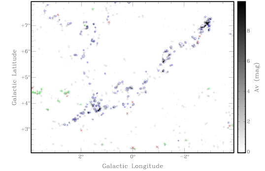
Figure 4: The ‘cores-only’, background-subtracted 2MASS visual extinction ($A_{V}$) image (Lombardi et al., 2006). Using the C¹⁸O (1–0)  emission toward each of the extinction peaks identified by clumpfind, we have determined which of the 201 extinction peaks are associated with dense gas, the Pipe Nebula, and if they are physically associated with any nearby extinction. Marked on this image are blue circles which correspond to the location and approximate extent of each of the 134 dense cores associated with the Pipe Nebula. The green plus symbols mark the extinction peaks that are associated with foreground/background molecular clouds. The red crosses mark the extinction peaks that had no detectable C¹⁸O (1–0)  emission.

Figure 5: Derived CMFs shown as binned histograms. The four panels correspond to different core samples when taking into consideration the C¹⁸O (1–0)  molecular line emission. Note that the shape of the mass function changes considerably when we use the C¹⁸O (1–0)  emission to guide the core extraction from the extinction image (i.e. between panels (a) and (d)). The dashed line corresponds to the scaled field star IMF of Muench et al. (2002). For each panel we determine, via a $\chi^{2}$ minimization, the offsets between the CMF and the IMF. To accurately determine these scaling factors, we minimize the $\chi^{2}$ between the distributions only for masses above the completeness limit. The derived parameters are summarized in Table 2. The vertical dotted line marks the mass completeness limit (Kainulainen et al., 2008). Included on the histograms are the errors for each bin (calculated as the square root of the number per bin).

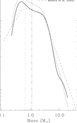
Figure 6: The improved CMF for the Pipe Nebula as a probability density function (solid curve) compared to the CMF of Alves et al. (2007) (dotted curve). The dashed line corresponds to the field star IMF of Muench et al. (2002) scaled up by a factor of $\sim$ 4.5. We interpret this difference in scaling to be a measure of the star formation efficiency (22 $\pm$ 8%) that will likely characterize the dense core population in the cloud at the end of the star formation process. The vertical dotted line marks the mass completeness limit, while the vertical dot-dashed line marks the fidelity limit (Kainulainen et al., 2008). We confirm earlier results that suggested that the Pipe CMF departs from a single power-law with a break at $\sim$ 2.7 $\pm$ 1.3  $M_{\odot}$.

References

- Alves et al. (2007) Alves, J., Lombardi, M., & Lada, C. J. 2007, A&A, 462, L17
- Enoch et al. (2008) Enoch, M. L., Evans, II, N. J., Sargent, A. I., Glenn, J., Rosolowsky, E., & Myers, P. 2008, ApJ, 684, 1240
- Johnstone & Bally (2006) Johnstone, D. & Bally, J. 2006, ApJ, 653, 383
- Johnstone et al. (2001) Johnstone, D., Fich, M., Mitchell, G. F., & Moriarty-Schieven, G. 2001, ApJ, 559, 307
- Johnstone et al. (2006) Johnstone, D., Matthews, H., & Mitchell, G. F. 2006, ApJ, 639, 259
- Johnstone et al. (2000) Johnstone, D., Wilson, C. D., Moriarty-Schieven, G., Joncas, G., Smith, G., Gregersen, E., & Fich, M. 2000, ApJ, 545, 327
- Kainulainen et al. (2008) Kainulainen, J., Alves, J. F., Lada, C. J., & Rathborne, J. M. 2008, A&A, submitted
- Kroupa (2001) Kroupa, P. 2001, MNRAS, 322, 231
- Lada et al. (2008) Lada, C. J., Muench, A. A., Rathborne, J., Alves, J. F., & Lombardi, M. 2008, ApJ, 672, 410
- Ladd et al. (2005) Ladd, N., Purcell, C., Wong, T., & Robertson, S. 2005, Publications of the Astronomical Society of Australia, 22, 62
- Lombardi et al. (2006) Lombardi, M., Alves, J., & Lada, C. J. 2006, A&A, 454, 781
- Motte et al. (1998) Motte, F., Andre, P., & Neri, R. 1998, A&A, 336, 150
- Motte et al. (2001) Motte, F., André, P., Ward-Thompson, D., & Bontemps, S. 2001, A&A, 372, L41
- Muench et al. (2007) Muench, A. A., Lada, C. J., Rathborne, J. M., Alves, J. F., & Lombardi, M. 2007, ApJ, 671, 1820
- Muench et al. (2002) Muench, A. A., Lada, E. A., Lada, C. J., & Alves, J. 2002, ApJ, 573, 366
- Nutter & Ward-Thompson (2007) Nutter, D. & Ward-Thompson, D. 2007, MNRAS, 374, 1413
- Onishi et al. (1999) Onishi, T., Kawamura, A., Abe, R., Yamaguchi, N., Saito, H., Moriguchi, Y., Mizuno, A., Ogawa, H., & Fukui, Y. 1999, PASJ, 51, 871
- Rathborne et al. (2008) Rathborne, J. M., Lada, C. J., Muench, A. A., Alves, J. F., & Lombardi, M. 2008, ApJS, 174, 396
- Reid & Wilson (2006a) Reid, M. A. & Wilson, C. D. 2006a, ApJ, 644, 990
- Reid & Wilson (2006b) —. 2006b, ApJ, 650, 970
- Silverman (1986) Silverman, B. W. 1986, Density estimation for statistics and data analysis (Monographs on Statistics and Applied Probability, London: Chapman and Hall, 1986)
- Simpson et al. (2008) Simpson, R. J., Nutter, D., & Ward-Thompson, D. 2008, ArXiv e-prints
- Smith et al. (2008) Smith, R. J., Clark, P. C., & Bonnell, I. A. 2008, MNRAS, 391, 1091
- Stanke et al. (2006) Stanke, T., Smith, M. D., Gredel, R., & Khanzadyan, T. 2006, A&A, 447, 609
- Swift & Williams (2008) Swift, J. J. & Williams, J. P. 2008, ApJ, 679, 552
- Testi & Sargent (1998) Testi, L. & Sargent, A. I. 1998, ApJ, 508, L91
- Williams et al. (1994) Williams, J. P., de Geus, E. J., & Blitz, L. 1994, ApJ, 428, 693
- Young et al. (2006) Young, K. E., Enoch, M. L., Evans, II, N. J., Glenn, J., Sargent, A., Huard, T. L., Aguirre, J., Golwala, S., Haig, D., Harvey, P., Laurent, G., Mauskopf, P., & Sayers, J. 2006, ApJ, 644, 326