Lévy flights in confining potentials

Abstract

We analyze confining mechanisms for Lévy flights. When they evolve in suitable external potentials their variance may exist and show signatures of a superdiffusive transport. Two classes of stochastic jump - type processes are considered: those driven by Langevin equation with Lévy noise and those, named by us topological Lévy processes (occurring in systems with topological complexity like folded polymers or complex networks and generically in inhomogeneous media), whose Langevin representation is unknown and possibly nonexistent. Our major finding is that both above classes of processes stay in affinity and may share common stationary (eventually asymptotic) probability density, even if their detailed dynamical behavior look different. That generalizes and offers new solutions to a reverse engineering (e.g. targeted stochasticity) problem due to I. Eliazar and J. Klafter [J. Stat. Phys. 111, 739, (2003)]: design a Lévy process whose target pdf equals a priori preselected one. Our observations extend to a broad class of Lévy noise driven processes, like e.g. superdiffusion on folded polymers, geophysical flows and even climatic changes.

I Introduction

The study of random walks in complex structures is a key point to understanding of properties of many physical and non-physical systems, ranging from transport in disordered media vank to transfer phenomena in biological cells and various real-world networks dor ; alb . It is well-known that a mean square displacement of a freely diffusing particle depends on time linearly $<X^{2}(t)>\propto t$. If a diffusion is anomalous, then $<X^{2}(t)>\propto t^{\gamma}$, where $\gamma\neq 1$, $0<\gamma<\infty$. If $\gamma<1$, the dynamics is called subdiffusive otherwise superdiffusive. A superdiffusive motion of a particle may be generated by means of non-Gaussian jump-type processes.

At this point one often invokes Lévy flights. Their free version may seem somewhat exotic since their second moments are nonexistent. However, Lévy flights in confining external potentials show up less exotic behavior and do admit the existence of first few moments (see, e.g., Ref. lev1 ). Thus they may be employed to model a superdiffusive transport.

Lévy flights, being non-Gaussian jump-type processes, quite apart from serious technical difficulties and a shortage of analytically tractable examples, occur in many fields of modern statistical physics and have won major attention in the last two decades lev1 -ditlevsen1 . Most of the current research is devoted to Langevin equation based derivations, where a deterministic force is perturbed by the (white) noise of interest, cufaro -dubkov . However, in a number of publications, another class of jump-type processes was introduced under the name of topologically induced super-diffusions, brockmann -geisel1 . The origin of this name is due to the fact that such processes occur primarily in the systems with topological complexity like folded polymers or complex networks. An observation of sokolov was that topological super-diffusion processes do not portray a situation equivalent to any of standard fractional Fokker-Planck equations and seem not to correspond to any Langevin equation. On the other hand, in the discussion of above topological Lévy processes main emphasis has been put on their super-diffusive behavior with some neglect of confining effects and the resultant emergence of non-Gibbsian stationary probability densities, brockmann -geisel1 .

We address the latter issue and set general confinement criteria for an analytically tractable case of Cauchy noise-driven processes. The results obtained appear to be more general and not specific to Cauchy noise. To this end, some ideas have been adopted from the general theory of diffusion-type stochastic processes where an asymptotic approach towards equilibrium (stationary probability density function (pdf)) is one of major topics of interest, mackey .

To handle topological Lévy processes we use a convenient and general mathematical tool, named Schrödinger (or Lévy - Schrödinger for non-Gaussian processes) semigroup. This tool naturally appears if one attempts to transform the evolution equation for the pdf $\rho$ of a certain stochastic process (e.g. standard or fractional Fokker- Planck equation), into the time - dependent Schrödinger- type equation (the parabolic one in the Gaussian context; there is no imaginary unit before time derivative) $\partial_{t}\psi={\mathcal{H}}\psi$. Here, $\mathcal{H}$ receives a natural interpretation of a Hamiltonian operator, $-\mathcal{H}$ stands for a semigroup generator. A proper exploitation of a semigroup operator $\exp(-t{\mathcal{H}})$ allows not only to generate the evolution equation for the pdf (differential or pseudo-differential in case of non-Gaussian Lévy noise, see below) but gives access to hitherto unexploited evolution scenarios which are not captured by the standard Langevin modeling.

We shall demonstrate that topologically induced processes of Refs. brockmann -geisel1 form a subclass of its solutions with a properly tailored dynamical semigroup and its (Feynman-Kac) potential, klauder ; olk . That allows to take advantage of the existing mathematical theory of Lévy processes and Lévy - Schrödinger semigroups, applebaum ; sato and klauder ; olk ; olk1 , where free Lévy noise generators are additively perturbed by suitable confining potentials. The theory works well for both Gaussian and non-Gaussian processes.

We note here, that in the Brownian case, the Schrödinger problem incorporates the well known transformation of a Fokker-Planck equation into a generalized diffusion equation, risken , e.g. a transition to the Hermitian (strictly speaking, self-adjoint) problem whose eigenfunction expansions yield transition pdfs of the pertinent process.

In this article, we consider an impact of external confining potentials upon Lévy flights. The flights may be influenced directly or indirectly (here via conservative forces) leading to inequivalent Lévy processes. An indirect influence refer to Langevin modeling, while a direct one refers the Lévy semigroups. While making this specific distinction between the two ways of response of Lévy noise to external potentials, we address an issue of an apparent incompatibility between them, raised earlier sokolov . The results obtained set a bridge between these seemingly different classes and may shed some light on the emergence of varied types of a superdiffusive dynamics in complex structures, especially those involving significant spatial inhomogeneities.

II Theoretical framework

II.1 Smoluchowski processes and Schrödinger semigroups

To make paper self-contained, here we recapitulate the main derivations, which will be necessary for us in subsequent discussion. We begin with consideration of a one-dimensional (1D) Smoluchowski diffusion process risken , with the Langevin representation $\dot{x}=b(x,t)+A(t)$, where $\langle A(s)\rangle=0$, $\langle A(s)A(s^{\prime})\rangle=2D\delta(s-s^{\prime})$. Here, $b(x,t)$ is a forward drift of the process, admitted to be time - dependent, unless we ultimately pass to Smoluchowski diffusion processes where $b(x,t)\equiv b(x)$ for all times.

If an initial pdf $\rho_{0}(x)$ is given, then the diffusion process drives it in accordance with the Fokker-Planck equation $\partial_{t}\rho=D\Delta\rho-\nabla\,(b\rho)$ (in the 1D case $\nabla\equiv\partial/\partial x$, $\Delta\equiv\partial^{2}/\partial x^{2}$). We introduce an osmotic velocity field $u=D\ln\rho$, together with the current velocity field $v=b-u$. The latter obeys the continuity equation $\partial_{t}\rho=-\nabla j$, where $j=v\cdot\rho$ has a standard interpretation of a probability current. The time-independent drifts $b(x)$ of the diffusion processes are induced by external (conservative, Newtonian) force fields $f=-\nabla V$. One arrives at Smoluchowski diffusion processes by setting

$$b={\frac{f}{m\beta}}=-{\frac{1}{m\beta}}\nabla V.$$ (1)

Here, $m$ is a mass and $\beta$ is a reciprocal relaxation time of a system. The expression (1) accounts for a fully - fledged phase - space derivation of the spatial process, in the regime of large $\beta$. It is taken for granted that the fluctuation-dissipation balance gives rise to the standard form $D=k_{B}T/m\beta$ of the diffusion coefficient $D$ ($T$ stands for a temperature and $k_{B}$ is Boltzmann constant).

Let us consider a stationary asymptotic regime, where $j\to j_{*}=0$. We denote an (a priori assumed to exist, mackey ), invariant pdf $\rho_{*}=\rho_{*}(x)$. Since in stationary case $v=v_{*}=0$, we have

$$b_{*}=u_{*}=D\nabla\ln\rho_{*}.$$ (2)

Since $b=f/m\beta$ does not depend on pdf explicitly, $b=b_{*}$ and $\rho_{*}(x)=(1/Z)\,\exp[-V(x)/k_{B}T]$. It is seen that our outcome has Gibbs-Boltzmann form with $Z$ being a partition function, $Z=\int\exp(-V/k_{B}T)\ dx$.

Denoting $F_{*}\equiv-k_{B}T\ln Z$, we have

$$\rho_{*}(x)=\exp\left([F_{*}-V(x)]/k_{B}T\right)\equiv\exp[2\Phi(x)]\,.$$ (3)

Here, to comply with the notations of Refs. zambrini; klauder and with subsequent discussion of a topological generalization of the Brownian motion and then Lévy flights brockmann -geisel1 , we have introduced a new potential function $\Phi$ such that $\rho_{*}^{1/2}=\exp(\Phi)$ and $b=2D\nabla\Phi$.

Following a standard procedure risken we transform the Fokker-Planck equation into an associated Hermitian problem by means of redefinition $\rho(x,t)=\theta^{*}(x,t)\exp[\Phi(x)]$, that takes the Fokker-Plack equation into a parabolic one risken $\partial_{t}\theta_{*}=D\Delta\theta_{*}-{\cal{V}}\theta_{*}$. Its potential ${\cal{V}}$ derives from a compatibility condition ${\cal{V}}(x)=(1/2)[b^{2}/(2D)+\nabla b]$.

Smoluchowski process with a unique asymptotic Gibbsian pdf implies

$${\cal{V}}=D\,{\frac{\Delta\rho_{*}^{1/2}}{\rho_{*}^{1/2}}}.$$ (4)

This equation is a trivialized version (due to the time- independence of its solution) of the time adjoint equation $\partial_{t}\theta=-D\Delta\theta+{\cal{V}}\theta$, see Refs.klauder ; olk setting $\theta=\rho_{*}^{1/2}$.

Introducing ($1/2mD$ rescaled) Schrödinger-type Hamiltonian ${\mathcal{H}}=-D\Delta+{\cal{V}}$, one arrives at a dynamical (Schrödinger) semigroup operator $\exp(-t{\mathcal{H}})$, with the dynamical rule $\theta^{*}(t)=[\exp(-t{\mathcal{H}})\theta^{*}](0)$, taking forward the initial data $\theta^{*}(x,0)$.

For completeness of discussion, we note that the time adjoint equation, if applicable, would come out from the reverse time evolution taking a given final (terminal) $\theta(x,t_{\rm fin})$ backwards in time to $\theta(x,t_{\rm fin}-t)=[\exp(-t{\mathcal{H}})\theta](t_{\rm fin})$, all motions being confined to an interval $[0,t_{\rm fin}]$.

II.2 Lévy - Schrödinger semigroups.

Before passing to an analysis of Lévy flights, let us set general rules of the game with respect to the response to external potentials, once a free noise is chosen. We recall that a characteristic function of a random variable $X$ completely determines a probability distribution of that variable. If this distribution admits a pdf $\rho(x)$, we can write $<\exp(ipX)>=\int_{R}\rho(x)\exp(ipx)dx$ which, for infinitely divisible probability laws, gives rise to the famous Lévy-Khintchine formula (see, e.g. applebaum )

$$<\exp(ipX)>=\exp\Biggl{\{}i\alpha p-(\sigma^{2}/2)p^{2}+$$

$$+\int_{-\infty}^{+\infty}\left[\exp(ipy)-1-{\frac{ipy}{1+y^{2}}}\right]\nu(dy)\Biggr{\}},$$ (5)

where $\nu(dy)$ stands for so-called Lévy measure. By disregarding the deterministic and jump-type contributions in the above, we are left with $<\exp(ipx)>=\exp(-\sigma^{2}p^{2}/2)$, hence $\rho(x)=(2\pi\sigma^{2})^{-1/2}\exp(-x^{2}/2\sigma^{2})$.

In terms of the random variable $X_{t}=(2D)^{1/2}A_{t}$ of the Wiener process, we have $<\exp(ipX_{t})>=\exp(-tDp^{2})$. By employing $p\to\hat{p}=-i\nabla$ we identify the semigroup operator $\exp(tD\Delta)$, with $\Delta=d^{2}/dx^{2}$. This involves a special version ${\mathcal{H}}=D\hat{p}^{2}=-D\Delta$ of the general Hamiltonian ${\mathcal{H}}=F(\hat{p})$.

From now on, we concentrate on the integral part of the Lévy-Khintchine formula, which is responsible for arbitrary stochastic jump features. By disregarding the deterministic and Brownian motion entries we arrive at:

$$F(p)=-\int_{-\infty}^{+\infty}\left[\exp(ipy)-1-\frac{ipy}{{1+y^{2}}}\right]\nu(dy),$$ (6)

where $\nu(dy)$ stands for the appropriate Lévy measure. The corresponding non-Gaussian Markov process is characterized by $<\exp(ipX_{t})>=\exp[-tF(p)]$ and yields an operator $F(\hat{p})={\mathcal{H}}$, with $\hat{p}=-i\nabla$.

For the sake of clarity we restrict further considerations to non-Gaussian random variables whose pdf’s are centered and symmetric, e.g. a subclass of stable distributions characterized by

$$F(p)=\lambda|p|^{\mu}\Rightarrow{\mathcal{H}}\equiv\lambda|\Delta|^{\mu/2}.$$ (7)

Here $\mu<2$ and $\lambda>0$ stands for the intensity parameter of the Lévy process. The fractional Hamiltonian ${\mathcal{H}}$, which is a non-local pseudo-differential operator, by construction is positive and self-adjoint on a properly tailored domain. A sufficient and necessary condition for both these properties to hold true is that the pdf of the Lévy process is symmetric, applebaum .

The associated jump-type dynamics is interpreted in terms of Lévy flights. In particular

$$F(p)=\lambda|p|\to{\mathcal{H}}=F(\hat{p})=\lambda|\nabla|\equiv\lambda(-\Delta)^{1/2}$$ (8)

refers to the Cauchy process, see e.g. klauder ; olk ; olk1 . The pseudo - differential Fokker-Planck equation, which corresponds to the fractional Hamiltonian (28) and the fractional semigroup $\exp(-t\hat{H}_{\mu})=\exp(-\lambda|\Delta|^{\mu/2})$, reads

$$\partial_{t}\rho=-\lambda|\Delta|^{\mu/2}\rho\,,$$ (9)

to be compared with the conventional heat equation $\partial_{t}\rho=D\Delta\rho$.

For a pseudo-differential operator $|\Delta|^{\mu/2}$, the action on a function from its domain is greatly simplified (as compared to Lévy-Khintchine formula (6)), in view of the properties of the Lévy measure $\nu_{\mu}(dx)$. We have klauder ; sokolov ; olk ; cufaro ; dubkov :

$$(|\Delta|^{\mu/2}f)(x)=-\int_{-\infty}^{\infty}[f(x+y)-f(x)]\nu_{\mu}(dy).$$ (10)

The Cauchy-Lévy measure, associated with the Cauchy semigroup generator $|\Delta|^{1/2}\equiv|\nabla|$, reads

$$\nu_{1/2}(dy)={\frac{1}{\pi}}{\frac{dy}{y^{2}}}.$$ (11)

The substitution $y\to z=x+y$ permits to reduce the Eq. (10) to the familiar form

$$(|\nabla|f)(x)=-\frac{1}{\pi}\int_{-\infty}^{\infty}{\frac{f(z)-f(x)}{|z-x|^{2}}}dz,$$ (12)

where $1/\pi|z-x|^{2}$ has an interpretation of an intensity with which jumps of the size $|z-x|$ occur.

III Response to external potentials: stationary densities

III.1 Langevin modeling

The pseudo-differential Fokker-Planck equation, which corresponds to the fractional Hamiltonian (7) and the fractional semigroup $\exp(-t{\mathcal{H}}_{\mu})=\exp(-t\lambda|\Delta|^{\mu/2})$, has the form (9) to be compared with the Fokker-Planck equation for freely diffusing particle (or above heat transfer equation) $\partial_{t}\rho=D\Delta\rho$.

In case of jump-type (Lévy) processes a response to external perturbations by conservative force fields appears to be particularly interesting. On one hand, one encounters a widely accepted reasoning (Refs. fogedby -dubkov ) where the Langevin equation, with additive deterministic and Lévy ”white noise” terms, is found to imply a fractional Fokker-Planck equation, whose form faithfully parallels the Brownian version, e.g. (c.f. Ref. fogedby , see also olk1 )

$$\dot{x}=b(x)+A^{\mu}(t)\Longrightarrow\partial_{t}\rho=-\nabla(b\cdot\rho)-\lambda|\Delta|^{\mu/2}\rho\,.$$ (13)

Here we make a remark regarding our notations. In 1D case operator $\nabla$ means simply differentiation over $x$ (see also above) so that all quantities like $f$ are scalars. In higher dimensions the operator $\nabla$, acting on vector quantity ${\vec{b}}\cdot\rho$ (${\vec{b}}\equiv-{\vec{\nabla}}V/m\beta$) should be understood as a vector divergence, i.e. the term ${\vec{\nabla}}({\vec{b}}\cdot\rho)$ $\equiv$ ${\rm{div}}({\vec{b}}\cdot\rho)$. Also, here we emphasize a difference in sign in the second term of Eq. (13) as compared to that in Eq. (4) of Ref. fogedby . There, the minus sign is absorbed in the adopted definition of the (Riesz) fractional derivative. Apart from the formal resemblance of operator symbols, we do not directly employ fractional derivatives in our formalism.

III.2 Topological route

The other approach to account for external perturbations is that, by mimicking the above Gaussian strategy, we can directly refer to the Hamiltonian framework and dynamical semigroups with Lévy generators being additively perturbed by a suitable potential. For example, assuming that the functional form of ${\cal{V}}(x)$ guarantees that ${\mathcal{H}}_{\mu}\equiv\lambda|\Delta|^{\mu/2}+{\cal{V}}$ is self-adjoint and bounded from below, we may pass to the fractional (non-Gaussian, jump process) analog of the generalized diffusion equation:

$$\partial_{t}\theta_{*}=-\lambda|\Delta|^{\mu/2}\theta_{*}-{\cal{V}}\theta_{*}.$$ (14)

The dynamical semigroup reads $\exp(-t{\mathcal{H}}_{\mu})$ and the compatibility condition related to Eq. (4), takes the form of the time-adjoint equation $\partial_{t}\theta=\lambda|\Delta|^{\mu/2}\theta+{\cal{V}}\theta$ gar2 . General theory klauder ; olk ; gar2 tells us that $\theta^{*}(x,t)\theta(x,t)=\rho(x,t)$ stands for a pdf of an affiliated Markov process that interpolates between the boundary data $\rho(x,0)$ and $\rho(x,t_{\rm fin})$, at times $t\in[0,t_{\rm fin}]$.

We consider time-independent $\theta(x,t)\equiv\theta(x)$ and hereby mimic the Gaussian ansatz: $\theta(x)=\exp[\Phi(x)]$ so that $\theta^{*}(x,t)=\rho(x,t)\,\exp[-\Phi(x)]$. If we set $\exp[\Phi(x)]=\rho^{1/2}_{*}(x)$, we get the compatibility condition (see Eq. (4)):

$${\cal{V}}=-\lambda\,{\frac{|\Delta|^{\mu/2}\,\rho^{1/2}_{*}}{\rho^{1/2}_{*}}}\,.$$ (15)

This identity should be compared with Eq. (8) in Ref. geisel , where an analogous effective potential was deduced in the study of Lévy flights in inhomogeneous media.

In view of the semigroup dynamics, we deduce a continuity equation with an explicit fractional input

$$\partial_{t}\rho=\theta\partial_{t}\theta^{*}=-\lambda(\exp\Phi)|\Delta|^{\mu/2}[\exp(-\Phi)\rho]+{\cal{V}}\cdot\rho.$$ (16)

Up to cosmetic changes $\Phi\to-V/2k_{B}T$ (compare with Eq. (3)), Eq. (16) is identical with transport equations employed in a number of papers. There, the investigated process was named a topologically induced superdiffusion. Namely, with respect to explicit form of Eq. (15), the Eq. (16) assumes a familiar form of the transport equation (with respect to $\lambda=1$ and $\kappa=1/(k_{B}T)$), see Eq. (6) in Ref. geisel , Eq. (5) in Ref. geisel1 and Eq. (36) in Ref. brockmann .

$$\partial_{t}\rho=-\exp(-\kappa V/2)\,|\Delta|^{\mu/2}\exp(\kappa V/2)\rho+\rho\exp(\kappa V/2)|\Delta|^{\mu/2}\exp(-\kappa V/2),$$ (17)

We note a systematic sign difference between our $|\Delta|^{\mu/2}$ and the corresponding fractional derivative $\Delta^{\mu/2}$ of Refs. brockmann ; geisel ; geisel1 .

III.3 A discord and the reverse engineering problem

The puzzling point is that for the Lévy process in external force fields, the Langevin approach yields a continuity (e.g. fractional Fokker-Planck) equation in a very different form

$$\partial_{t}\rho=-\nabla\left(-{\frac{\nabla V}{m\beta}}\,\rho\right)-\lambda|\Delta|^{\mu/2}\rho\,.$$ (18)

The conclusion of Refs. brockmann -geisel1 was that, while assuming $\Phi\sim V$ where $V$ is (up to inessential factors) the above external force potential, the two transport equations (16) and (18) are plainly incompatible so that Eq. (16) seems not correspond to any Langevin equation with Lévy noise term and $b=-\nabla V/m\beta$ as a deterministic part and vice versa. This puzzling discrepancy has not been explored previously in more depth.

The problem we address is:

(i)

choose a functional form of $V(x)$ and thus the drift of the Langevin - type process;

(ii)

infer an invariant pdf $\rho_{*}$ that is compatible with the fractional Fokker-Planck equation (18);

(iii)

given $\rho_{*}$, deduce the Feynman-Kac (e.g. dynamical semigroup) potential ${\cal{V}}$ by means of Eq. (15);

(iv)

use ${\cal{V}}$ in (16) and verify whether the ”topologically induced dynamics” is at all related to that associated with (18) (and thus to the underlying Langevin equation with Lévy noise);

(v)

check an asymptotic behavior of $\rho(x,t)$ in both scenarios (16) and (18) to find possible differences in the speed (convergence time rate) with which the common invariant pdf $\rho_{*}(x)$ from item (ii) is approached;

(vi)

repeat the procedure in reverse order by starting from step (iii) and then deduce the drift for the Langevin equation with Lévy noise; next compare the dynamical scenarios (16) and (18) for any common initial pdf.

We recall that the the above problem is non-existent in the case of Brownian motion. There, the Fokker-Planck dynamics and the related parabolic equations do refer to the same diffusion-type process.

We shall demonstrate below that both Langevin - driven and semigroup - driven Cauchy processes, albeit non - coinciding literally, keep resemblance to each other and may share common for both stationary pdf. A superdiffusive dynamical behavior is generically expected to arise and an asymptotic approach towards a stationary pdf is then in principle possible. This motivates the ”targeted stochasticity” discussion whose original formulation (in terms of the reverse engineering problem) for Langevin - driven Lévy systems can be found in Ref. klafter . The original formulation of the reverse engineering problem reads: given a stationary pdf, can we tailor a drift function so that the system Langevin dynamics would admit the predefined as an asymptotic target?

We employ the reverse engineering problem to analyze Cauchy processes in confining potentials. In the course of the discussion, we in fact extend its range of applicability (that applies to more general stable processes as well) and demonstrate that a priori chosen stationary pdf may serve as a target density for both Langevin and semigroup - driven Cauchy processes. Even though their detailed dynamical patterns of behavior are different. In the near - equilibrium regime this dynamical distinction becomes immaterial.

IV Cauchy driver

In view of serious technical difficulties we shall not attempt to present a fully fledged solution to the above formulated problem for any symmetric stable jump-type process and any conceivable drift. Instead, we turn our attention to situations where explicit functional forms of invariant densities are available. Most of them were inferred in the problems, related to Cauchy noise, see Refs klauder ; olk1 , fogedby -dubkov . In particular, attention has been paid to confining properties of various drifts upon the Cauchy noise. On the other hand, Lévy flights through a ”potential landscape” (topological processes of Refs. brockmann -geisel1 ) were interpreted as (enhanced) super-diffusions.

IV.1 Ornstein - Uhlenbeck - Cauchy process

Let us consider the Ornstein - Uhlenbeck - Cauchy (OUC) process, whose drift is given by $b(x)=-\gamma x$, and an asymptotic invariant pdf associated with the Cauchy-Fokker-Planck equation $\partial_{t}\rho=-\lambda|\nabla|\rho+\nabla[(\gamma x)\rho]$ reads

$$\rho_{*}(x)=\frac{\sigma}{\pi}\frac{1}{\sigma^{2}+x^{2}},\ \sigma=\frac{\lambda}{\gamma},$$ (19)

c.f. Eq. (9) in Ref. olk1 . Here, the modified noise intensity parameter $\sigma$ is a ratio of an intensity parameter $\lambda$ of the Cauchy noise and of the friction coefficient $\gamma$. Note that a characteristic function of this pdf reads $F(p)=-\sigma|p|$ and accounts for a non-thermal fluctuation-dissipation balance.

For Cauchy random variable $X_{t}$ we have $\langle\exp(ipX_{t})\rangle$ = $\exp(t\lambda|p|)$. The corresponding pdf has the form (19) with $\sigma\sim t\lambda$, e.g. $\rho(x,t)=\lambda t/\pi[(\lambda t)^{2}+x^{2}]$. Here, $\sigma$ and $t\lambda$ play a role of scaling parameters specifying the half-width of the Cauchy pdf at its half-maximum. Since $t\lambda$ grows monotonically, the free Cauchy noise pdf flattens and its maximum drops down in time.

Since $\sigma=\lambda/\gamma$, the confining drift $-\gamma x$ may stop the ”flattening” of the probability distribution and stabilize the pdf at quite arbitrary shape (with respect to its maximum and half-width, see above), by manipulating $\gamma$. For example, $\gamma\gg 1$ implies a significant shrinking of the distribution $\rho_{*}$ as compared to the reference (free noise) pdf at any time $t\sim 1/\lambda$. In parallel, a maximum pdf value would increase: $1/\pi\lambda\to\gamma/\pi\lambda$.

The OUC case refers to Cauchy flights in a confining (harmonic) potential, but does not imply the confined flight, since the variance of the asymptotic density diverges. We note that confined Lévy flights and specifically confined Cauchy flights, have been analyzed earlier in Refs. chechkin -dubkov .

To deduce the potential ${\cal{V}}$ for the OUC process with given invariant pdf $\rho_{*}$, we need to evaluate the right-hand-side of the defining Eq. (15), with $\mu=1$. We employ Eq. (12), so arriving at:

$$\frac{\pi}{\lambda}\frac{1}{(\sigma^{2}+x^{2})^{1/2}}\,{\cal{V}}(x)=$$

$$=\int_{-\infty}^{\infty}\left[{\frac{1}{\sqrt{\sigma^{2}+(x+y)^{2}}}}-{\frac{1}{\sqrt{\sigma^{2}+x^{2}}}}\right]{\frac{dy}{y^{2}}}.$$ (20)

Because of the integrand singularity at $y=0$, we must handle the integral in terms of its principal value. Introducing the notation $a=\sigma^{2}+x^{2}$, we arrive at, gradstein :

$${\cal{V}}(x)={\frac{\lambda}{\pi}}\left[-{\frac{2}{\sqrt{a}}}+{\frac{x}{a}}\ln{\frac{\sqrt{a}+x}{\sqrt{a}-x}}\right].$$ (21)

Here, ${\cal{V}}(x)$ is bounded both from below and above, with the asymptotics $(2/|x|)\ln|x|$ at infinities, well fitting to the general mathematical construction of (topological) Cauchy processes in external potentials, see Ref. olk for details. The plot of potential (21) is reported in Fig.1.

Accordingly, we know for sure that there exists a topological Cauchy process with the Feyman - Kac potential ${\cal{V}}$, Eq. (21), whose invariant density coincides with that for the Langevin - supported OUC process.

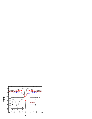
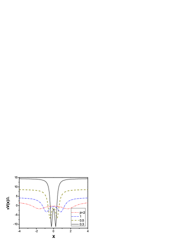
Figure 1: The coordinate dependence of potentials ${\cal{V}}(x)$: (21) for different $\sigma$ (main left panel), (24) (inset to left panel) and (35) for different $\beta$ (right panel).

IV.2 Confined Cauchy processes: Langevin and topological targeting

To analyze a time-dependent behavior of both topological and Langevin - driven process, below we consider specific numerical example, admitting finite variance $<X^{2}(t)>$. This time dependent variance permits to analyze a particular scenario of approaching the invariant (equilibrium) density in the large time regime. We will see, that two considered jump - type processes, whose time evolution is embodied respectively in the fractional Fokker-Planck equation and in Lévy-Schrödinger semigroup (topological case) dynamics are definitely alike as they share a common invariant density. In the near-equilibrium regime, any dynamical distinction between these motion scenarios becomes immaterial. However, their detailed dynamical behavior far from equilibrium might be different and this issue deserves further analytical and numerical exploration.

To our current knowledge, there is no Langevin - type representation of a topological process and vice versa, even though an invariant density is common for both. Nonetheless, we will demonstrate that by starting from a common initial probability density, the two (Langevin and dynamical semigroup) motion scenarios end up at a common invariant density.

Neither OUC process nor its topological counterpart are confined. For the Cauchy density, the second moment is nonexistent. We shall verify the outcome of the OUC discussion for Cauchy-type processes whose invariant densities admit the second moment due to confinement. Let us consider the quadratic Cauchy pdf:

$$\rho_{*}(x)=\frac{2}{\pi}\frac{1}{(1+x^{2})^{2}}$$ (22)

Now, let us proceed in reverse order departing from Eq. (22), so that $(1/\sqrt{2\pi})\rho_{*}^{1/2}=(1/\pi)/(1+x^{2})$ is actually Cauchy pdf. We consider $f(x)=\rho_{*}^{1/2}$ as the initial data for the free Cauchy evolution $\partial_{t}f=\lambda|\nabla|f$. This takes $f(x)$ into the form

$$f(x,t)=\sqrt{\frac{2}{\pi}}\,{\frac{1+\lambda t}{(1+\lambda t)^{2}+x^{2}}}.$$ (23)

Since $\lambda|\nabla|f=-\lim_{t\to 0}\partial_{t}f$ we end up with

$${\cal{V}}(x)={\frac{\lim_{t\to 0}\partial_{t}f}{f}}(x)=\lambda{\frac{x^{2}-1}{x^{2}+1}}\,.$$ (24)

The shape of this potential is shown in Fig.1 (inset to left panel). A minimum $-\lambda$ is achieved at $x=0$, ${\cal{V}}=0$ occurs for $x=\pm 1$, a maximum $+\lambda$ is reached at $x\to\pm\infty$.

The potential is bounded both from below and above and hence can trivially be made non-negative (add $\lambda$). This means that the potential (24) is fully compatible with the general construction of Ref, olk . This topological process is generated by Cauchy generator plus a potential function, see Ref. olk , is of the jump-type and can be obtained as an $\epsilon\to 0$ limit of a step process with a minimal step size $\epsilon$.

Note, that in Ref. olk no explicit example of the confining potential ${\cal{V}}$ has been proposed. Eqs. (21), (24) provide such examples, which, to our knowledge, have never been exploited in the literature.

At this point, let us make a guess that the quadratic Cauchy pdf actually stands for an invariant pdf of the ”normal” Langevin-based fractional Fokker-Planck equation (18) with a drift of the form (1). Accordingly we should have $\partial_{t}\rho_{*}=0=-\nabla(b\,\rho_{*})-\gamma|\nabla|\rho_{*}$ and therefore the admissible drift function, if any, may be deduced by means of an indefinite integral:

$$b(x)=-{\frac{\gamma}{\rho_{*}(x)}}\int(|\nabla|\rho_{*})(x)\,dx.$$ (25)

For quadratic Cauchy pdf (22) the explicit form of $b(x)$ (25) reads

$$b(x)=-\frac{\gamma x}{8}(x^{2}+3).$$ (26)

Thus, there exists the Langevin process whose invariant pdf is shared with a corresponding topological process. In the near - equilibrium regime a dynamical distinction between the pertinent processes becomes immaterial. In other words, if we wish to deal with the Langevin process associated with the quadratic Cauchy density (22), the proper drift form is given in (26).

To analyze numerically the above apparent discord between Langevin-driven and topological processes, we use the invariant pdf (22), having drift (26) and Feynman - Kac potential (24). We have chosen this invariant pdf as it has a finite variance, which permits us to capture the details of near - equilibrium, initial and intermediate stages of time evolution.

For numerical solution we use simple Euler scheme for time derivatives and numerical integration (more specifically, we calculate Cauchy principal value of integrals) on the each Euler time step for evaluation of fractional derivative $|\nabla|$. The initial state corresponds to a particle localized at $x=0$, corresponding to the minima of both potential, derived from the drift (26) and Feynman - Kac potential (24), $\rho(x,t=0)=\delta(x)$. The solutions $\rho(x,t)$ of the equations (18) (Langevin-type process) and (17) (topological process) are reported in Fig.2 (upper and middle panels respectively).

It is seen that topological diffusion process needs more time to achieve the invariant pdf, appears to be slowed down as compared to the Langevin scenario. This is illustrated in Fig. 2 (lower panel), where the time evolution of variances for both processes have been plotted. The time evolution occurs from zero variance of $\delta$ function to asymptotic variance $<X^{2}(t\to\infty)>=1$ of the pdf (22). It is seen, that variance for Langevin - type process achieves the asymptotic value at (dimensionless) time $t\approx 0.5$, while for topological diffusion this time $t\approx 2$. The shapes of $<X^{2}(t)>$ for both processes definitely resemble a super - diffusive motion.

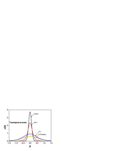
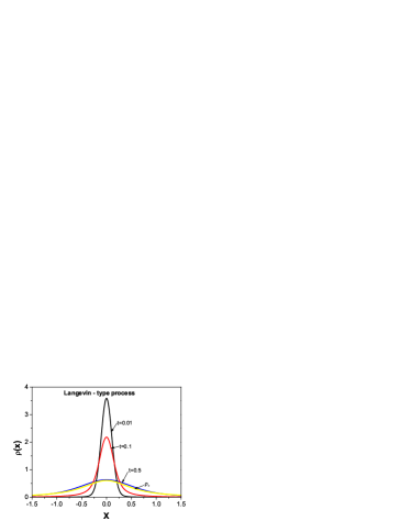
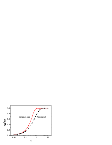
Figure 2: Time evolution of pdf’s $\rho(x,t)$ for topological (upper panel, $\lambda=1$) and Langevin-type (middle panel, $\beta=1$, $m=1$) processes. The common equilibrium pdf $\rho_{*}$ (22) is also shown. Lower panel reports the time dependent variance $X^{2}(t)$ for Langevin-type (solid line) and topological (dashed line) processes. Points correspond to numerical calculation, lines are guides for eye.

IV.3 Confined Cauchy family

Now we consider a broader class of pdf’s related to the Cauchy noise. Any continuous pdf $\rho$ can be associated with Shannon entropy $S(\rho)=-\int\rho\,\ln\rho\,dx$, kapur . If an expectation value $<\ln(1+x^{2})>$ is fixed, the maximum entropy probability function belongs to a one-parameter family

$$\rho_{*}(x)={\frac{\Gamma(\alpha)}{\sqrt{\pi}\Gamma(\alpha-1/2))}}\,{\frac{1}{(1+x^{2})^{\alpha}}}$$ (27)

where $\alpha>1/2$, kapur .

Cauchy distribution is a special case of the above $\rho_{*}$ that corresponds to $\alpha=1$. The density (22) is the second, $\alpha=2$, member of the $\alpha$ - integer hierarchy (we assume that $\sigma=1$).

Our tentative analysis shows that for integer and half - integer $\alpha$, the invariant pdf (27) admits ${\cal{V}}(x)$, which fits the restrictions of Corollary 2 in Ref. olk . The question about arbitrary $\alpha$ is still under investigation.

For each specific function ${\cal{V}}(x)$, the resulting Markov jump-type stochastic process, determined by the Cauchy generator plus a suitable potential function, appears to be unique. Here we present only one specific example, namely we consider

$$\rho_{*}(x)={\frac{16}{5\pi}}\,{\frac{1}{(1+x^{2})^{4}}}.$$ (28)

Substitution of Eq. (28) into Eq. (15) with respect to definition (12) yields gradstein the following expression for the Feynman-Kac (semigroup) potential

$${\cal{V}}(x)=\frac{\gamma}{2}\frac{x^{4}+6x^{2}-3}{1+x^{2}}.$$ (29)

The potential is bounded from below, its minimum at $x=0$ equals $-3\gamma/2$. For large values of $|x|$, the potential behaves as $\sim(\gamma/2)x^{2}$ i.e. demonstrates a harmonic behavior.

Apart from the unboundedness of ${\cal{V}}(x)$ from above, this potential obeys the minimal requirements of Corollary 2 in Ref. olk : can be made positive (add a suitable constant), is locally bounded (e.g. is bounded on each compact set) and is measurable (e.g. can be approximated with arbitrary precision by step functions sequences). The Cauchy generator plus the potential (29) determine uniquely an associated Markov process of the jump-type and its step process approximations.

Having the density (28), we can readily address the problem (vi) of Section III.3. Namely, inserting Eq. (28) to Eq. (25), we obtain

$$b(x)=-{\frac{\gamma x}{16}}\,(5x^{6}+21x^{4}+35x^{2}+35).$$ (30)

This function shows a linear friction $b\sim-x$ for small $x$ and a strong taming behavior $b\sim-x^{7}$ for large $x$.

Let us finally consider a bimodal pdf (see, e.g. Ref. dubkov )

$$\rho_{*}(x)=\frac{\beta^{3}}{\pi}\frac{1}{x^{4}-\beta^{2}x^{2}+\beta^{4}},$$ (31)

which is a solution of so-called quartic Cauchy oscillator. As a form of the (confining) potential $V(x)\propto x^{4}$ is known for that pdf, we can check the correctness of the procedure (25) of deriving a drift (and hence the potential $V(x)$ in Langevin scenario) for this pdf. The application of operator (12) to function (31) yields

$$|\nabla|\rho_{*}(x)=\frac{\pi x^{2}}{\beta^{3}}\frac{x^{4}+\beta^{2}x^{2}-3\beta^{4}}{(x^{4}-\beta^{2}x^{2}+\beta^{4})^{2}},$$ (32)

which after integration over $x$ and division over $\rho_{*}(x)$ (31) yields

$$b(x)=-\gamma\frac{x^{3}}{\beta^{3}},$$ (33)

$$V(x)=-\int b(x)dx=\frac{\gamma}{4\beta^{3}}x^{4},$$ (34)

which is exactly the form of the potential for quartic Cauchy oscillator. The expression (31) can also be used to calculate the ”topological” potential ${\cal V}(x)$

$${\cal V}(x)=\frac{\lambda}{\pi}\sqrt{x^{4}-\beta^{2}x^{2}+\beta^{4}}\int\limits_{-\infty}^{\infty}{\frac{{dy}}{{y^{2}}}\left[{\frac{1}{{\sqrt{(x+y)^{4}-\beta^{2}(x+y)^{2}+\beta^{4}}}}-\frac{1}{{\sqrt{x^{4}-\beta^{2}x^{2}+\beta^{4}}}}}\right]}.$$ (35)

Since an analytic outcome has proved not to be tractable, we have reiterated to numerics. The result of numerical calculation of the function (35) is reported in Fig 1 (right panel) for different $\beta$. It is seen that this potential is also bounded from below and above, can be made non - negative and have all properties imposed by Corollary 2 of Ref. olk .

V Conclusions

Explicitly solvable models are scarce in theoretical studies of Lévy flights, especially in the presence of external potentials and/or external conservative forces. Therefore, our major task was to find novel analytically tractable examples, that would shed some light on apparent discrepancies between dynamical patterns of behavior associated with two different fractional transport equations that are met in the literature on Lévy flights.

Although the predominant part of this research is devoted to the standard Langevin modeling, we have demonstrated that so - called topological Lévy processes form a subclass of solutions to the Schrödinger boundary data problem. The pertinent dynamical behavior stems form a suitable Lévy - Schrödinger semigroup. The crucial role of the involved Feynman - Kac potential has been identified. We have explicitly derived these potential functions in a number of cases.

The major gain of above observations is that a mathematical theory of Ref. olk tells one what are the necessary functional properties of admissible Feynman-Kac potentials. Their proper choice makes a topological Lévy process a well behaved mathematical construction, with a well defined Markovian dynamics and stationary pdf.

Our focus was upon confinement mechanisms that tame Lévy flights to the extent that second moments of their probability densities exist. We have shown that the dynamical behavior of both above classes of processes are close to each other in the near-equilibrium regime and admit common (for both classes) stationary pdf. This pdf, in turn, determines a functional form of the aforementioned (semigroup defining) potential function.

We have generalized the reverse engineering (targeted stochasticity) problem of Ref. klafter beyond the original Lévy - Langevin processes setting. We have demonstrated, that within the targeted stochasticity framework, the concept of Lévy flights in confining potentials is not limited to the standard Langevin scenario. The Lévy - Schrödinger semigroup explicitly involves confining potentials, but with no obvious link to a Langevin representation. Our version of the reverse engineering problem amounts to reconstructing from a given (target) stationary density the potential functions that either: (i) define the forward drift of the Langevin process, or (ii) enter the Schrödinger - type Hamiltonian expression in the semigroup dynamics. Both dynamical scenarios are expected to yield the same asymptotic outcome i.e. the preselected target pdf.

We note that a departure point for our investigation was a familiar transformation of the Fokker - Planck operator into its Hermitian (Schrödinger - type) counterpart, undoubtedly valid in the Gaussian case. The Fokker - Planck and the corresponding parabolic equation (plus a compatibility condition) essentially describe the same random dynamics. An analogous transformation is non - existent for non - Gaussian processes. Two fractional transport equations discussed in the present paper are inequivalent in the non - Gaussian case so that the semigroup and the Langevin dynamics with the Lévy driver (e.g. noise) refer to different random processes. The reverse engineering problem allowed us to demonstrate that those two processes may nevertheless share the same target pdf and close near equilibrium behavior.

Since the Schrödinger boundary data problem allows for a construction of an interpolating Markovian processes between any two a priori prescribed probability densities, it is of interest to fix an initial pdf and choose an invariant pdf as an asymptotic (terminal) datum. That is why in the present paper we have given a detailed comparison of a temporal behavior of the Langevin - based and topological process, both sharing the same invariant pdf.

- (1) N.G. van Kampen, Stochastic Processes in Physics and Chemistry. (North-Holland, Amsterdam, 1981).
- (2) S.N. Dorogovtsev and J.F.F. Mendes, Evolution of Networks: From Biological Nets to the Internet and WWW. (Oxford University Press, Oxford, 2003).
- (3) R. Albert and A.-L. Barabási, Rev. Mod. Phys. 74, 47, (2002).
- (4) Lévy Flights and Related Topics in Physics, Lecture Notes in Physics, edited by M. F. Shlesinger, G.M. Zaslavsky, and U. Frisch (Springer-Verlag, Berlin, 1995); c.f. also Chaos: The interplay between deterministic and stochastic behavior, edited by P. Garbaczewski, M. Wolf and A. Weron, (Springer-Verlag, Berlin, 1995)
- (5) P. Garbaczewski, J. R. Klauder and R. Olkiewicz, Phys. Rev. E 51, 4114, (1995).
- (6) V. V. Belik and D. Brockmann, New. J. Phys. 9, 54, (2007).
- (7) D. Brockmann and I. Sokolov, Chem. Phys. 284, 409, (2002)
- (8) D. Brockmann and T. Geisel, Phys. Rev. Lett. 90, 170601, (2003)
- (9) D. Brockmann and T. Geisel, Phys. Rev. Lett. 91, 048303, (2003)
- (10) H. Risken, The Fokker-Planck equation, Springer-Verlag, Berlin, 1989
- (11) P. Garbaczewski and R. Olkiewicz, J. Math. Phys. 40, 1057, (1999)
- (12) P. Garbaczewski and R. Olkiewicz, J. Math. Phys. 41, 6843, (2000)
- (13) N. Cufaro Petroni and M. Pusterla, Physica A 388, 824, (2009)
- (14) D. Applebaum, Lévy processes and stochastic calculus. Cambridge University Press, 2004
- (15) K-I. Sato, Lévy processes and infinitely divisible distributions, Cambridge University Press, 1999
- (16) P. Garbaczewski, arxiv:0902.3536 (2009)
- (17) S. Jespersen, R. Metzler and H. C. Fogedby, Phys. Rev. E 59, 2736, (1999)
- (18) P. D. Ditlevsen, Phys. Rev. E 60, 172, (1999)
- (19) V. V. Janovsky et al., Physica A 282, 13, (2000)
- (20) A. A. Dubkov, B. Spagnolo and V. V. Uchaikin, Int. J. Bifurcations and Chaos, 18, 2549, (2008)
- (21) P. D. Ditlevsen, Geophys. Res. Lett. 26, 1441, (1999)
- (22) M. C. Mackey and M. Tyran-Kamińska, J. Stat. Phys. 124, 1443-1470, (2006)
- (23) I. Eliazar and J. Klafter, J. Stat. Phys. 111, 739, (2003)
- (24) I. S. Gradshteyn and I. M. Ryzhik, Table of integrals, series and products, Academic Press, NY, 2007
- (25) J. N. Kapur and H. K. Kesavan, Entropy Optimization Principles with Applications, Academic Press, Boston, 1992