Approche variationnelle pour le calcul bay sien dans les probl mes inverses en imagerie

Résumé

Dans une approche bay sienne non supervis e pour la r solution d’un probl me inverse, on cherche estimer conjointement la grandeur d’int r t ${\mathb{f}}$ et les param tres ${\boldsymbol{\theta}}$ partir des donn es observ es ${\mathb{g}}$ et un mod le ${\mathcal{M}}$ liant ces grandeurs. Ceci se fait en utilisant la loi a posteriori conjointe $p({\mathb{f}},{\boldsymbol{\theta}}|{\mathb{g}};{\mathcal{M}})$. L’expression de cette loi est souvent complexe et son exploration et le calcul des estimateurs bay siens n cessitent soit les outils d’optimisation de crit res ou de calcul d’esp rances des lois multivari es. Dans tous ces cas, il y a souvent besoin de faire des approximations. L’approximation de Laplace et les m thodes d’ chantillonnage MCMC sont deux approches classiques (analytique et num rique) qui ont t explor s avec succ s pour ce fin. Ici, nous tudions l’approximation de $p({\mathb{f}},{\boldsymbol{\theta}}|{\mathb{g}})$ par une loi s parable en ${\mathb{f}}$ et en ${\boldsymbol{\theta}}$. Ceci permet de proposer des algorithmes it ratifs plus abordables en co t de calcul, surtout, lorsqu’on choisit ces lois approchantes dans des familles des lois exponentielles conjugu es. Le principal objet de ce papier est de pr senter les diff rents algorithmes que l’on obtient pour diff rents choix de ces familles. À titre d’illustration, nous consid rons le cas de la restauration d’image par d convolution simple ou myope avec des a priori s parables, markoviens simples ou avec des champs cach s.

Approche variationnelle pour le calcul bay sien dans les probl mes inverses en imagerie

Abstract

In a non supervised Bayesian estimation approach for inverse problems in imaging systems, one tries to estimate jointly the unknown image pixels ${\mathb{f}}$ and the hyperparameters ${\boldsymbol{\theta}}$ given the observed data ${\mathb{g}}$ and a model ${\mathcal{M}}$ linking these quantities. This is, in general, done through the joint posterior law $p({\mathb{f}},{\boldsymbol{\theta}}|{\mathb{g}};{\mathcal{M}})$. The expression of this joint law is often very complex and its exploration through sampling and computation of the point estimators such as MAP and posterior means need either optimization of or integration of multivariate probability laws. In any of these cases, we need to do approximations. Laplace approximation and sampling by MCMC are two approximation methods, respectively analytical and numerical, which have been used before with success for this task. In this paper, we explore the possibility of approximating this joint law by a separable one in ${\mathb{f}}$ and in ${\boldsymbol{\theta}}$. This gives the possibility of developing iterative algorithms with more reasonable computational cost, in particular, if the approximating laws are choosed in the exponential conjugate families. The main objective of this paper is to give details of different algorithms we obtain with different choices of these families. To illustrate more in detail this approach, we consider the case of image restoration by simple or myopic deconvolution with separable, simple markovian or hidden markovian models.

1 Introduction

Une pr sentation simplifi e et synth tique des probl mes inverses en imagerie, en se pla ant en dimensions finies, consiste vouloir retrouver une grandeur inconnue ${\mathb{f}}$ partir des observations ${\mathb{g}}$ d’une grandeur observ e, en supposant conna tre un mod le ${\mathcal{M}}$ qui les lient. La forme la plus simple de ce mod le est un mod le lin aire de la forme

$${\mathcal{M}}:\qquad{\mathb{g}}={\mathb{H}}{\mathb{f}}+{\boldsymbol{\epsilon}}$$ (1)

o on suppose que toutes les erreurs de mod lisation et de mesure peuvent tre repr sent es par ${\boldsymbol{\epsilon}}$. Notons aussi que ${\mathb{g}}$ et ${\mathb{f}}$ sont, en g n ral, des vecteurs de grandes dimensions, ce qui signifie que nous consid rons ici le cas discr tis o ${\mathb{g}}$ contient l’ensemble des grandeurs mesur es et ${\mathb{f}}$ l’ensemble des valeurs qui d crivent la grandeur inconnue. Dans ce contexte ${\mathb{H}}$ est une matrice dont les l ments sont d finies par le mod le et les tapes de discr tisation du probl me.

Dans une approche estimation bay sienne non supervis e pour r soudre un probl me inverse, d’abord on utilise ce mod le pour d finir la loi de probabilit $p({\mathb{g}}|{\mathb{f}},{\boldsymbol{\theta}}_{1};{\mathcal{M}})$ o ${\boldsymbol{\theta}}_{1}$ repr sente l’ensemble des param tres qui d crivent cette loi. Lors que cette fonction est consid r e comme une fonction de ${\mathb{f}}$ et de ${\boldsymbol{\theta}}_{1}$, elle est appel e la vraisemblance des inconnues ${\mathb{f}}$ et ${\boldsymbol{\theta}}$ du mod le ${\mathcal{M}}$. Son expression s’obtient partir de la loi de probabilit des erreurs ${\boldsymbol{\epsilon}}$ en utilisant le mod le (1). Par exemple, lorsque ${\boldsymbol{\epsilon}}$ dans ce mod le est mod lis par un vecteur al atoire centr , blanc, gaussien et de covariance fix e ${\boldsymbol{\Sigma}}_{\epsilon}={\sigma_{\epsilon}}^{2}{\mathb{I}}$, on a

$$p({\mathb{g}}|{\mathb{f}},{\boldsymbol{\theta}}_{1};{\mathcal{M}})={\mathcal{N}}({\mathb{H}}{\mathb{f}},{\boldsymbol{\Sigma}}_{\epsilon})$$ (2)

o ${\boldsymbol{\theta}}_{1}={\sigma_{\epsilon}}^{2}$. D’autres lois avec d’autres param tres ${\boldsymbol{\theta}}_{1}$ peuvent bien s r tre utilis es.

La deuxi me tape dans cette approche est l’attribution ou le choix d’une loi dite a priori $p({\mathb{f}}|{\boldsymbol{\theta}}_{2};{\mathcal{M}})$ pour les inconnues ${\mathb{f}}$, o ${\boldsymbol{\theta}}_{2}$ repr sente ses param tres. La troisi me tape consiste crire l’expression de la loi a posteriori des inconnues ${\mathb{f}}$ :

$$p({\mathb{f}}|{\boldsymbol{\theta}},{\mathb{g}};{\mathcal{M}})=\frac{p({\mathb{g}},{\mathb{f}}|{\boldsymbol{\theta}};{\mathcal{M}})}{p({\mathb{g}}|{\boldsymbol{\theta}};{\mathcal{M}})}=\frac{p({\mathb{g}}|{\mathb{f}},{\boldsymbol{\theta}}_{1};{\mathcal{M}})\;p({\mathb{f}}|{\boldsymbol{\theta}}_{2};{\mathcal{M}})}{p({\mathb{g}}|{\boldsymbol{\theta}};{\mathcal{M}})},$$ (3)

o on suppose implicitement conna tre l’ensemble des param tres ${\boldsymbol{\theta}}=({\boldsymbol{\theta}}_{1},{\boldsymbol{\theta}}_{2})$. Mais, dans un cas r el, nous sommes amen s souvent les estimer aussi. Pour cela, dans l’approche bay sienne, on leur attribue aussi une loi a priori $p({\boldsymbol{\theta}}|{\mathcal{M}})$, et l’on obtient alors une loi a posteriori conjointe des inconnues ${\mathb{f}}$ et des hyperparam tres ${\boldsymbol{\theta}}=({\boldsymbol{\theta}}_{1},{\boldsymbol{\theta}}_{2})$ :

$$p({\mathb{f}},{\boldsymbol{\theta}}|{\mathb{g}};{\mathcal{M}}) = \frac{p({\mathb{g}},{\mathb{f}},{\boldsymbol{\theta}}|{\mathcal{M}})}{p({\mathb{g}}|{\mathcal{M}})}$$ (4)

$$= \frac{p({\mathb{g}}|{\mathb{f}},{\boldsymbol{\theta}}_{1};{\mathcal{M}})\;p({\mathb{f}}|{\boldsymbol{\theta}}_{2};{\mathcal{M}})\;p({\boldsymbol{\theta}}|{\mathcal{M}})}{p({\mathb{g}}|{\mathcal{M}})}.$$

Dans cette relation, le d nominateur

$$p({\mathb{g}}|{\mathcal{M}})=\int\kern-8.00003pt\int p({\mathb{g}}|{\mathb{f}},{\boldsymbol{\theta}};{\mathcal{M}})\;p({\mathb{f}}|{\boldsymbol{\theta}};{\mathcal{M}})\;p({\boldsymbol{\theta}}|{\mathcal{M}})\mbox{\leavevmode\nobreak\ d}{\mathb{f}}\mbox{\leavevmode\nobreak\ d}{\boldsymbol{\theta}}$$ (5)

est la vraisemblance marginale du mod le ${\mathcal{M}}$ dont son logarithme $\ln p({\mathb{g}}|{\mathcal{M}})$ est appell vidence du mod le ${\mathcal{M}}$.

Afin d’introduire les notions qui vont tre utilis es dans la suite de ce travail, il est int ressant de mentionner que, pour n’importe quelle loi de probabilit $q({\mathb{f}},{\boldsymbol{\theta}})$ (dont nous verrons le choix et l’utilit par la suite), l’ vidence du mod le $\ln p({\mathb{g}}|{\mathcal{M}})$ v rifie

$$\ln p({\mathb{g}}|{\mathcal{M}}) = \ln\int\kern-8.00003pt\int p({\mathb{g}},{\mathb{f}},{\boldsymbol{\theta}}|{\mathcal{M}})\mbox{\leavevmode\nobreak\ d}{\mathb{f}}\mbox{\leavevmode\nobreak\ d}{\boldsymbol{\theta}}$$ (6)

$$= \ln\int\kern-8.00003pt\int q({\mathb{f}},{\boldsymbol{\theta}})\frac{p({\mathb{g}},{\mathb{f}},{\boldsymbol{\theta}}|{\mathcal{M}})}{q({\mathb{f}},{\boldsymbol{\theta}})}\mbox{\leavevmode\nobreak\ d}{\mathb{f}}\mbox{\leavevmode\nobreak\ d}{\boldsymbol{\theta}}$$

$$\geq \int\kern-8.00003pt\int q({\mathb{f}},{\boldsymbol{\theta}})\ln\frac{p({\mathb{g}},{\mathb{f}},{\boldsymbol{\theta}}|{\mathcal{M}})}{q({\mathb{f}},{\boldsymbol{\theta}})}\mbox{\leavevmode\nobreak\ d}{\mathb{f}}\mbox{\leavevmode\nobreak\ d}{\boldsymbol{\theta}}.$$

(d’apr s l’in galit de Jensen : $\ln(\mbox{E}\left\{p/q\right\})\geq\mbox{E}\left\{\ln(p/q)\right\}$). Aussi, notant par

$${\mathcal{F}}(q)=\int\kern-8.00003pt\int q({\mathb{f}},{\boldsymbol{\theta}})\ln\frac{p({\mathb{g}},{\mathb{f}},{\boldsymbol{\theta}}|{\mathcal{M}})}{q({\mathb{f}},{\boldsymbol{\theta}})}\mbox{\leavevmode\nobreak\ d}{\mathb{f}}\mbox{\leavevmode\nobreak\ d}{\boldsymbol{\theta}}$$ (7)

et par

$$\mbox{KL}(q:p)=\int\kern-8.00003pt\int q({\mathb{f}},{\boldsymbol{\theta}})\ln\frac{q({\mathb{f}},{\boldsymbol{\theta}})}{p({\mathb{f}},{\boldsymbol{\theta}}|{\mathb{g}};{\mathcal{M}})}\mbox{\leavevmode\nobreak\ d}{\mathb{f}}\mbox{\leavevmode\nobreak\ d}{\boldsymbol{\theta}}$$ (8)

on montre facilement (en rempla ant $p({\mathb{g}},{\mathb{f}},{\boldsymbol{\theta}}|{\mathcal{M}})=p({\mathb{f}},{\boldsymbol{\theta}}|{\mathb{g}};{\mathcal{M}})\;p({\mathb{g}}|{\mathcal{M}})$ dans l’expression de ${\mathcal{F}}(q)$) que

$$\ln p({\mathb{g}}|{\mathcal{M}})={\mathcal{F}}(q)+\mbox{KL}(q:p).$$ (9)

Ainsi ${\mathcal{F}}(q)$, appel e l’ nergie libre de $q({\mathb{f}},{\boldsymbol{\theta}})$ par rapport $p({\mathb{g}},{\mathb{f}},{\boldsymbol{\theta}}|{\mathcal{M}})$, est une limite inf rieure de $\ln p({\mathb{g}}|{\mathcal{M}})$ car $\mbox{KL}(q:p)\geq 0$. Par la suite, nous allons crire l’expression de ${\mathcal{F}}(q)$ par

$${\mathcal{F}}(q)=\left<\ln{p({\mathb{g}},{\mathb{f}},{\boldsymbol{\theta}};{\mathcal{M}})}\right>_{q}+{\mathcal{H}}(q)$$ (10)

o nous avons utilis la notation $<.>_{q}$ pour l’esp rance suivant la loi $q$ et ${\mathcal{H}}(q)$ est l’entropie de $q$ :

$$H(q)=-\int\kern-8.00003pt\int q({\mathb{f}},{\boldsymbol{\theta}})\ln{q({\mathb{f}},{\boldsymbol{\theta}})}\mbox{\leavevmode\nobreak\ d}{\mathb{f}}\mbox{\leavevmode\nobreak\ d}{\boldsymbol{\theta}}$$ (11)

Arriv ce stade, les questions pos es sont :

• Inf rence : Étant donn e les expressions des lois a posteriori (3) et (4), comment les utiliser pour d finir une solution au probl me inverse d crit en (1) ?

• S lection de mod le : Comment peut-on s lectionner un mod le parmi un ensemble de mod les ${\mathcal{M}}_{i}$.

En ce qui concerne le probl me de l’inf rence, les principaux choix sont les estimateurs au sens du Maximum a posteriori (MAP) ou au sens de la moyenne a posteriori (PM). Dans le premier cas, on a besoin des outils d’optimisation et dans le deuxi me cas des outils d’int gration (analytique ou num rique). Pour la s lection du mod le, nous nous contenterons ici de noter que l’expression de la vraisemblance du mo le (5) peut tre utilis s cette fin. Dans ce papier, nous nous focalisons sur la premi re question o on cherche inf rer ${\mathb{f}}$ et ${\boldsymbol{\theta}}$ utilisant la loi a posteriori jointe (4).

Pour les probl mes inverses, la solution au sens du MAP a t utilis e avec succ s pour sa simplicit et en raison de son lien avec l’approche d terministe de la r gularisation. Mais, il y a des situations o cette solution ne donne pas satisfaction, et o la solution au sens de la moyenne a posteriori peut tre pr f r e. Mais, les situations o on peut avoir une solution analytique pour les int grations qui sont n cessaires pour obtenir ces estim es sont rares. Il y a alors pratiquement deux voies :

Int gration num rique par chantillonnage : Il s’agit d’approcher les esp rances par des moyennes empiriques des chantillons g n r s suivant la loi a posteriori . Toute la difficult est alors de g n rer ces chantillons, et c’est l qu’interviennent les m thodes de MCMC (Markov Chain Mont Carlo). Le principal int r t de ces m thodes est qu’elles permettent d’explorer l’ensemble de l’espace de la loi a posteriori , mais l’inconv nient majeur est leur co t de calcul qui est d au nombre important d’it rations n cessaire pour la convergence des cha nes et le nombre important de points qu’il faut g n rer pour obtenir des estimations de bonnes qualit s.

Approximation de la loi a posteriori par des lois plus simples : Il s’agit de reporter le calcul des int grales apr s une simplification par approximation de la loi a posteriori . Une premi re approximation utilis e historiquement est Approximation de Laplace o on approxime la lois a posteriori par une loi gaussienne. Dans ce cas, les deux estimateurs MAP et PM sont quivalents et tous les calculs deviennent analytiques.

Une deuxi me solution est d’approcher la a posteriori par une loi s parable, ce qui permet de r duire la dimension des int grations. Cette voie est plus r cente et le principal objet de ce papier.

De fa on g n rale, l’id e d’approcher une loi conjointe $p({\mathb{x}})$ de plusieurs variables ${\mathb{x}}$ par une loi s parable $q({\mathb{x}})=\prod_{j}q_{j}(x_{j})$ n’est pas nouveau et peut tre trouv e dans la litt ratures de la fin des ann es 90: [1, 2, 3, 4, 5, 6, 7]. Le choix d’un crit re pour mesurer la qualit de cette approximation et l’ tude des effets de cette approximation sur les qualit s des estimateurs obtenus appara t dans les travaux plus r cents [8, 9, 10, 11, 12, 13, 14, 15, 16, 17, 18, 19]. L’usage de cette approche en estimation des param tres d’un mod le d’observation avec des variables cach es en statistique est galement r cente [20, 19, 21, 22, 23, 24, 25, 26, 27, 28, 29, 30, 31, 32, 33, 34, 35]. Dans la plupart de ces travaux, l’application est plut t en classification en utilisant un mod le de m langes. Dans le domaine du traitement du signal, ils utilisent des mod les de m lange avec des tiquettes des classes mod lis es par des cha nes de Markov. Dans le domaine du traitement d’image, la plupart de ces travaux sont consacr s la segmentation d’image en utilisant soit un mod le s parable ou markovien pour les tiquettes. Cette approche a t aussi utilis r cemment en s paration de sources [36, 37, 38] et en traitement des images hyperspectrales [39, 40]. L’application r elle de cette approche pour simplifier les calculs bay siens dans les probl mes inverses avec un op rateur m langeant est l’originalit de ce travail [41, 42, 43]. En effet, dans la plupart de ces travaux, avec les notations utilis es dans ce papier, on suppose qu’on a observ directement ${\mathb{f}}$ dont la loi est mod lis e par un m lange de gaussiennes et le principal objectif de ces m thodes est l’estimation des param tres de ce m lange et la s lection du mod le. Dans d’autres travaux on consid re un mod le d’observation ponctuel o $g_{i}=h(f_{i})+\epsilon_{i}$ et l’objective est la segmentation de l’image ${\mathb{f}}$. Les travaux dans lesquels, on utilise l’approche variationnelle pour des probl mes inverses de restauration ou de reconstruction d’images sont assez rare. On trouve essentiellement les travaux [44, 45, 46] qui consid rent le cas des probl mes inverses lin aires, mais soit avec des mod les a priori de Gauss-Markov ou avec des variables cach es de contours ou d’ tiquettes des r gions s parables. La d pendance spatiale de ces variables cach es n’est pas prise en compte.

La suite de ce papier est organis e de la mani re suivante : une pr sentation tr s synth tique de l’approche variationnelle est fournie dans la section 2. Dans la section 3, nous nous int resserons l’approximation de la loi a posteriori $p({\mathb{f}},{\boldsymbol{\theta}}|{\mathb{g}};{\mathcal{M}})$ pour les probl mes inverses. Il s’agit alors d’appliquer l’approche variationnelle pour ce cas particulier avec diff rent choix pour les familles des lois approchantes. Dans la section 4, nous d taillerons l’application de la m thode au cas de la restauration simple ou myope d’image. Enfin, dans la section 5, nous d crirons la mani re d’appliquer cette m thode au cas de la restauration d’image avec une mod lisation a priori plus complexe : un mod le hi rarchique de Gauss-Markov avec un champ cach de Potts pour des tiquettes des r gions dans l’image. En effet, cette mod lisation convient pour bien des cas de restauration et de reconstruction d’images dans des applications o l’image recherch e repr sente un objet compos d’un nombre fini de mat riaux homog nes. C’est exactement cette information a priori qui est mod lis e par un mod le de m lange avec des tiquettes ${\mathb{z}}$ markoviennes [47]. Ici, donc, la loi a posteriori $p({\mathb{f}},{\mathb{z}},{\boldsymbol{\theta}}|{\mathb{g}};{\mathcal{M}})$ doit tre approxim e par des lois plus simples utiliser. Finalement, dans la section 6, nous r sumons les apports de ce papier. Il est noter cependant, que dans ce papier, seules les principes des m thodes propos es sont pr sent s et les d tails de mise en oeuvre de ces m thodes, ainsi que des r sultats de simulations et valuation des performances de ces algorithmes sont report es un prochaine papier.

2 Principe de l’approche variationnelle

Consid rons le probl me g n ral de l’approximation d’une loi conjointe $p({\mathb{x}}|{\mathcal{M}})$ de plusieurs variables ${\mathb{x}}$ par une loi s parable $q({\mathb{x}})=\prod_{j}q_{j}(x_{j})$. videment, il faut choisir un crit re. Consid rons le crit re de divergence $\mbox{KL}(q:p)$ entre $p$ et $q$ :

$$\mbox{KL}(q:p)=\int\kern-11.00008pt\int q({\mathb{x}})\ln\frac{q({\mathb{x}})}{p({\mathb{x}}|{\mathcal{M}})}\mbox{\leavevmode\nobreak\ d}{\mathb{x}}$$

et cherchons la solution $\widehat{q}({\mathb{x}})$ qui le minimise. La solution optimale ne peut tre calcul e que d’une mani re it rative, car ce crit re n’ tant pas quadratique en $q$, sa d riv e par rapport $q$ n’est pas lin aire et une solution explicite n’est pas disponible. On peut alors envisager une solution it rative coordonn e par coordonn e.

Notons $q_{-j}({\mathb{x}}_{-j})=\prod_{i\not=j}q_{i}(x_{i})$, ce qui permet d’ crire $q({\mathb{x}})=q_{j}(x_{j})\,q_{-j}({\mathb{x}}_{-j})$ o ${\mathb{x}}_{-j}=\{x_{i},i\not=j\}$ et d v loppons ce crit re :

$$\mbox{KL}(q:p) = -\int\kern-11.00008pt\int q({\mathb{x}})\ln\frac{p({\mathb{x}}|{\mathcal{M}})}{q({\mathb{x}})}\mbox{\leavevmode\nobreak\ d}{\mathb{x}}$$ (12)

$$= -H(q)-\left<\ln p({\mathb{x}}|{\mathcal{M}})\right>_{q({\mathb{x}})}$$

$$= -\sum_{j}H(q_{j})-\left<\ln p({\mathb{x}}|{\mathcal{M}})\right>_{q({\mathb{x}})}$$

$$= -\sum_{j}H(q_{j})-\int\left<\ln p({\mathb{x}}|{\mathcal{M}})\right>_{q_{-j}}q_{j}(x_{j})\mbox{\leavevmode\nobreak\ d}x_{j}$$

o $H(q)$ est l’entropie de $q$ et $H(q_{j})$ est l’entropie de $q_{j}$.

Notons que si $q_{-j}$ est fix e $\mbox{KL}(q:p)$ est convexe en $q_{j}$ et sa minimisation sous la contrainte de normalisation de $q_{j}$ s’ crit

$$q_{j}(x_{j})=\frac{1}{C_{j}}\exp\left[{\left<\ln p({\mathb{x}}|{\mathcal{M}})\right>_{q_{-j}}}\right]$$ (13)

avec

$$C_{j}=\int\exp\left[{\left<\ln p({\mathb{x}}|{\mathcal{M}})\right>_{q_{-j}}}\right]\mbox{\leavevmode\nobreak\ d}x_{j}$$ (14)

On note que l’expression de $q_{j}$ d pend de celle de ${q_{-j}}$ et que, l’obtention de $q_{j}$ ( tant donn e $q_{-j}$) se fait aussi d’une mani re it rative en deux tapes :

$$\left\{\begin{array}[]{ll}{\mathcal{Q}}(q_{j})&=H(q_{j})+\left<\ln p({\mathb{x}}|{\mathcal{M}})\right>_{q_{j})},\\ q_{j}^{(k+1)}&=\arg\max_{q_{j}}\left\{{\mathcal{Q}}(q_{j})\right\},\end{array}\right.$$ (15)

ce qui ressemble un algorithme du type EM (Esp rance-Maximisation) g n ralis , car dans la premi re quation nous avons calculer une esp rance et dans la deuxi me tape nous avons une maximisation.

Les calculs non param triques sont souvent trop co teux. On choisit alors une forme param trique pour ces lois de telle sorte que l’on puisse, chaque it ration, remettre jour seulement les param tres de ces lois, condition cependant que ces formes ne changent pas au cours des it rations. La famille des lois exponentielles conjugu es ont cette propri t [2, 44, 48, 49, 50, 51, 30].

La premi re tape de simplification de ce calcul est donc de consid rer la famille des lois param triques $q_{j}(x_{j}|{\boldsymbol{\theta}}_{j})$ o ${\boldsymbol{\theta}}_{j}$ est un vecteur de param tres. En effet, dans ce cas, l’algorithme it ratif pr c dent se transforme  :

$$\left\{\begin{array}[]{ll}{\mathcal{Q}}({\boldsymbol{\theta}}_{j})&=H\left(q_{j}(x_{j}|{\boldsymbol{\theta}}_{j})\right)+\left<\ln p({\mathb{x}}|{\mathcal{M}})\right>_{q_{j}(x_{j}|{\boldsymbol{\theta}}_{j})},\\ {\boldsymbol{\theta}}_{j}^{(k+1)}&=\arg\max_{{\boldsymbol{\theta}}_{j}}\left\{{\mathcal{Q}}({\boldsymbol{\theta}}_{j})\right\},\end{array}\right.$$ (16)

ce qui ressemble plus un algorithme du type EM.

Une deuxi me tape de simplification est de choisir pour $p({\mathb{x}}|{\boldsymbol{\theta}};{\mathcal{M}})$ la famille des lois exponentielles conjugu es :

$$p({\mathb{x}}|{\boldsymbol{\theta}};{\mathcal{M}})=f({\mathb{x}})\,g({\boldsymbol{\theta}})\,\exp\left[{{\boldsymbol{\phi}}({\boldsymbol{\theta}})^{T}{\mathb{u}}({\mathb{x}})}\right]$$ (17)

o ${\boldsymbol{\phi}}({\boldsymbol{\theta}})$ est le vecteur de param tres naturel et $f({\mathb{x}})$, $g({\boldsymbol{\theta}})$ et ${\mathb{u}}({\mathb{x}})$ sont des fonctions connues. Il est alors facile de montrer que $q_{j}(x_{j})$ dans l’ quation (13) sera aussi dans la famille des lois exponentielles conjugu es, et par cons quence $q({\mathb{x}}|\widetilde{{\boldsymbol{\theta}}})$ restera dans la m me famille et nous aurons juste remettre jours ses param tres.

Remarque : Cette famille de lois a une propri t dite conjugu e dans le sens que si on choisit comme a priori

$$p({\boldsymbol{\theta}}|\eta,\mbox{\boldmath$\nu$})=h(\eta,\mbox{\boldmath$\nu$})\,g({\boldsymbol{\theta}})^{\eta}\,\exp\left[{\mbox{\boldmath$\nu$}^{T}{\boldsymbol{\phi}}({\boldsymbol{\theta}})}\right]$$ (18)

l’a posteriori correspondant

$$p({\boldsymbol{\theta}}|{\mathb{x}};{\mathcal{M}})\propto p({\mathb{x}}|{\boldsymbol{\theta}};{\mathcal{M}})\;p({\boldsymbol{\theta}}|\eta,\mbox{\boldmath$\nu$})$$ (19)

sera aussi dans la m me famille (18). La famille des lois a priori (17) est alors dites conjugu e de la famille des lois (16).

Pour cette famille de lois, on a

$$\left<\ln p({\mathb{x}}|{\boldsymbol{\theta}};{\mathcal{M}})\right>_{q}=\left<\ln f({\mathb{x}})\right>_{q}+\ln g({\boldsymbol{\theta}})+{\boldsymbol{\phi}}({\boldsymbol{\theta}})^{T}\left<{\mathb{u}}({\mathb{x}})\right>_{q}$$ (20)

et donc la forme de la loi s parable $q_{j}$ correspondante est

$$q_{j}(x_{j}|\widetilde{{\boldsymbol{\theta}}})\propto g(\widetilde{{\boldsymbol{\theta}}})\exp\left[{<f({\mathb{x}})>_{q_{{}_{j}}}+{\boldsymbol{\phi}}(\widetilde{{\boldsymbol{\theta}}})^{T}<{\mathb{u}}({\mathb{x}})>_{q_{{}_{j}}}}\right]$$ (21)

o $\widetilde{{\boldsymbol{\theta}}}$ d signe les param tres particuliers de $q_{j}$ qu’il faut mettre jour au cours des it rations.

Par ailleurs, sachant que $q({\mathb{x}})$ est s parable, si $\ln p({\mathb{x}}|{\boldsymbol{\theta}};{\mathcal{M}})$ est polynomial en ${\mathb{x}}$, le calcul de l’esp rance (20), mais surtout celui de sa d riv e par rapport aux $q_{j}$ et aux param tres ${\boldsymbol{\theta}}$, qui sont n cessaire pour l’optimisation, seront facilit s. Comme nous le verrons par la suite, pour les probl mes inverses, nous avons choisi ce genre de lois.

3 Approche variationnelle pour les probl mes inverses lin aires

Nous allons maintenant utiliser ces relations pour d crire le principe de l’approche variationnelle au cas particulier des probl mes inverses (1) o l’utilisation directe de la loi a posteriori conjointe $p({\mathb{f}},{\boldsymbol{\theta}}|{\mathb{g}};{\mathcal{M}})$ dans l’ quation (4) est souvent trop co teuse pour pouvoir tre explor e par chantillonnage direct de type Mont Carlo ou pour calculer les moyennes a posteriori

$$\widehat{{\mathb{f}}}=\int\int{\mathb{f}}\;{p({\mathb{f}},{\boldsymbol{\theta}}|{\mathb{g}};{\mathcal{M}})}\mbox{\leavevmode\nobreak\ d}{\boldsymbol{\theta}}\mbox{\leavevmode\nobreak\ d}{\mathb{f}}$$ (22)

et

$$\widehat{{\boldsymbol{\theta}}}=\int\int{\boldsymbol{\theta}}\;{p({\mathb{f}},{\boldsymbol{\theta}}|{\mathb{g}};{\mathcal{M}})}\mbox{\leavevmode\nobreak\ d}{\mathb{f}}\mbox{\leavevmode\nobreak\ d}{\boldsymbol{\theta}}.$$ (23)

En effet, rare sont les cas o on puisse trouver d’expressions analytiques pour ces int grales. De m me l’exploration de cette loi par des m thodes de Mont Carlo est aussi co teuses. On cherche alors l’approcher par une loi plus simple $q({\mathb{f}},{\boldsymbol{\theta}})$. Par simplicit , nous entendons par exemple une loi $q$ qui soit s parable en ${\mathb{f}}$ et en ${\boldsymbol{\theta}}$ :

$$q({\mathb{f}},{\boldsymbol{\theta}})=q_{1}({\mathb{f}})\;q_{2}({\boldsymbol{\theta}})$$ (24)

videmment, cette approximation doit tre faite de telle sorte qu’une mesure de distance entre $q$ et $p$ soit minimale. Si, d’une mani re naturelle, on choisi $\mbox{KL}(q:p)$ comme cette mesure, on aura:

$$(\widehat{q}_{1},\widehat{q}_{2})=\arg\min_{(q_{1},q_{2})}\left\{\mbox{KL}(q_{1}q_{2}:p)\right\}=\arg\max_{(q_{1},q_{2})}\left\{{\mathcal{F}}(q_{1}q_{2})\right\}$$ (25)

et sachant que $\mbox{KL}(q_{1}q_{2}:p)$ est convexe en $q_{1}$ $q_{2}$ fix e et vice versa, on peut obtenir la solution d’une mani re it rative :

$$\left\{\begin{array}[]{ll}\widehat{q}_{1}&=\arg\min_{q_{1}}\left\{\mbox{KL}(q_{1}\widehat{q}_{2}:p)\right\}=\arg\max_{q_{1}}\left\{{\mathcal{F}}(q_{1}\widehat{q}_{2})\right\};\\ \widehat{q}_{2}&=\arg\min_{q_{2}}\left\{\mbox{KL}(\widehat{q}_{1}q_{2}:p)\right\}=\arg\max_{q_{2}}\left\{{\mathcal{F}}(\widehat{q}_{1}q_{2})\right\}.\end{array}\right.$$ (26)

Utilisant la relation (7), il est facile de montrer que les solutions d’optimisation de ces tapes sont

$$\left\{\begin{array}[]{ll}\widehat{q}_{1}({\mathb{f}})&\propto\exp\left[{\left<\ln{p({\mathb{g}},{\mathb{f}},{\boldsymbol{\theta}};{\mathcal{M}})}\right>_{\widehat{q}_{2}({\boldsymbol{\theta}})}}\right]\\ \widehat{q}_{2}({\boldsymbol{\theta}})&\propto\exp\left[{\left<\ln{p({\mathb{g}},{\mathb{f}},{\boldsymbol{\theta}};{\mathcal{M}})}\right>_{\widehat{q}_{1}({\mathb{f}})}}\right]\end{array}\right.$$ (27)

Une fois cet algorithme converg vers $\widehat{q}^{*}_{1}({\mathb{f}})$ et $\widehat{q}^{*}_{2}({\boldsymbol{\theta}})$, on peut les utiliser d’une mani re ind pendante pour calculer, par exemple les moyennes  $\widehat{{\mathb{f}}}^{*}=\int{\mathb{f}}\;\widehat{q}^{*}_{1}({\mathb{f}})\mbox{\leavevmode\nobreak\ d}{\mathb{f}}$  et
$\widehat{{\boldsymbol{\theta}}}^{*}=\int{\boldsymbol{\theta}}\;\;\widehat{q}^{*}_{2}({\boldsymbol{\theta}})\mbox{\leavevmode\nobreak\ d}{\boldsymbol{\theta}}$.

Comme nous l’avons d j indiqu , les calculs non param triques sont souvent trop co teux. On choisit alors une forme param trique pour ces lois de telle sorte que l’on puisse, chaque it ration, remettre jour seulement les param tres de ces lois. Nous examinons ici, trois cas:

3.1 Cas d g n r

On prend pour $q_{1}({\mathb{f}})$ et $q_{2}({\boldsymbol{\theta}})$ des formes d g n r es suivantes :

$$\left\{\begin{array}[]{ll}q_{1}({\mathb{f}}|\widetilde{{\mathb{f}}})&=\delta({\mathb{f}}-\widetilde{{\mathb{f}}})\\ q_{2}({\boldsymbol{\theta}}|\widetilde{{\boldsymbol{\theta}}})&=\delta({\boldsymbol{\theta}}-\widetilde{{\boldsymbol{\theta}}})\end{array}\right.$$ (28)

Par cons quence, au cours des it rations, nous n’aurons qu’ remettre jour $\widetilde{{\mathb{f}}}$ et $\widetilde{{\boldsymbol{\theta}}}$. En rempla ant $q_{1}({\mathb{f}})$ et $q_{2}({\boldsymbol{\theta}})$ dans les relations (27) on obtient :

$$\left\{\begin{array}[]{ll}\widehat{q}_{1}({\mathb{f}})\propto p({\mathb{g}},{\mathb{f}},\widetilde{{\boldsymbol{\theta}}};{\mathcal{M}})\propto p({\mathb{f}},\widetilde{{\boldsymbol{\theta}}}|{\mathb{g}};{\mathcal{M}})\\ \widehat{q}_{2}({\boldsymbol{\theta}})\propto p({\mathb{g}},\widetilde{{\mathb{f}}},{\boldsymbol{\theta}};{\mathcal{M}})\propto p(\widetilde{{\mathb{f}}},{\boldsymbol{\theta}}|{\mathb{g}};{\mathcal{M}}).\end{array}\right.$$ (29)

Il est alors facile de voir que la recherche de $\widetilde{{\mathb{f}}}$ et $\widetilde{{\boldsymbol{\theta}}}$ au cours des it rations devient quivalent  :

$$\left\{\begin{array}[]{@{}l@{}l@{}l@{}}\widetilde{{\mathb{f}}}&=\arg\max_{{\mathb{f}}}\left\{p({\mathb{g}},{\mathb{f}},\widetilde{{\boldsymbol{\theta}}};{\mathcal{M}})\right\}&=\arg\max_{{\mathb{f}}}\left\{p({\mathb{f}},\widetilde{{\boldsymbol{\theta}}}|{\mathb{g}};{\mathcal{M}})\right\}\\ \widetilde{{\boldsymbol{\theta}}}&=\arg\max_{{\boldsymbol{\theta}}}\left\{p({\mathb{g}},\widetilde{{\mathb{f}}},{\boldsymbol{\theta}};{\mathcal{M}})\right\}&=\arg\max_{{\boldsymbol{\theta}}}\left\{p(\widetilde{{\mathb{f}}},{\boldsymbol{\theta}}|{\mathb{g}};{\mathcal{M}})\right\}\end{array}\right.$$ (30)

On remarque alors que l’on retrouve un algorithme de type MAP joint ou ICM (Iterated Conditional Mode). L’inconv nient majeur ici est qu’avec le choix (28), les incertitudes li es chacune des inconnues ${\mathb{f}}$ et ${\boldsymbol{\theta}}$ ne sont pas prise en compte pour l’estimation de l’autre inconnue.

3.2 Cas particulier conduisant l’algorithme EM

On prend comme dans le cas pr c dent une forme d g n r e pour $q_{2}({\boldsymbol{\theta}})=\delta({\boldsymbol{\theta}}-\widetilde{{\boldsymbol{\theta}}})$, ce qui donne

$$\widehat{q}_{1}({\mathb{f}})\propto p({\mathb{g}},{\mathb{f}},\widetilde{{\boldsymbol{\theta}}};{\mathcal{M}})\propto p({\mathb{f}},\widetilde{{\boldsymbol{\theta}}}|{\mathb{g}};{\mathcal{M}})\propto p({\mathb{f}}|\widetilde{{\boldsymbol{\theta}}},{\mathb{g}};{\mathcal{M}})$$ (31)

ce qui signifie que $\widehat{q}_{1}({\mathb{f}})$ est une loi dans la m me famille que la loi a posteriori $p({\mathb{f}}|{\boldsymbol{\theta}},{\mathb{g}};{\mathcal{M}})$. Évidemment, si la forme de cette loi est simple, par exemple une gaussienne, (ce qui est le cas dans les situations que nous tudierons) les calculs seront simples.

A chaque it ration, on aurait alors remettre jour $\widetilde{{\boldsymbol{\theta}}}$ qui est ensuite utilis pour trouver $\widehat{q}_{1}({\mathb{f}}|\widetilde{{\boldsymbol{\theta}}})=p({\mathb{f}}|\widetilde{{\boldsymbol{\theta}}},{\mathb{g}};{\mathcal{M}})$, elle m me utilis e pour calculer

$$Q({\boldsymbol{\theta}},\widetilde{{\boldsymbol{\theta}}})=\left<\ln{p({\mathb{g}},{\mathb{f}},{\boldsymbol{\theta}};{\mathcal{M}})}\right>_{\widehat{q}_{1}({\mathb{f}}|\widetilde{{\boldsymbol{\theta}}})}.$$ (32)

On remarque facilement l’ quivalence avec l’algorithme EM qui se r sume  :

$$\left\{\begin{array}[]{@{}l@{}l@{}l@{}}\mbox{E\leavevmode\nobreak\ :\leavevmode\nobreak\ \leavevmode\nobreak\ }Q({\boldsymbol{\theta}},\widetilde{{\boldsymbol{\theta}}})&=\left<\ln{p({\mathb{g}},{\mathb{f}},{\boldsymbol{\theta}};{\mathcal{M}})}\right>_{\widehat{q}_{1}({\mathb{f}}|\widetilde{{\boldsymbol{\theta}}})},\\ \mbox{M\leavevmode\nobreak\ :\leavevmode\nobreak\ \leavevmode\nobreak\ }\widetilde{{\boldsymbol{\theta}}}&=\arg\max_{{\boldsymbol{\theta}}}\left\{Q({\boldsymbol{\theta}},\widetilde{{\boldsymbol{\theta}}})\right\}.\end{array}\right.$$ (33)

L’inconv nient majeur ici est que l’incertitude li e ${\boldsymbol{\theta}}$ n’est pas prise en compte pour l’estimation de ${\mathb{f}}$.

3.3 Choix particulier propos pour les probl mes inverses lin aires

Il s’agit de choisir, pour $q_{1}({\mathb{f}})$ et $q_{2}({\boldsymbol{\theta}})$ des lois dans les m mes familles de lois que celles de $p({\mathb{f}}|{\mathb{g}},{\boldsymbol{\theta}})$ et de $p({\boldsymbol{\theta}}|{\mathb{g}},{\mathb{f}})$. En effet, comme nous le verrons plus bas, dans le cas des probl mes inverses lin aires (1) avec des choix appropri pour les lois a priori associ e la mod lisation directe du probl me, ces lois a posteriori conditionnelles restes dans les m mes familles, ce qui permet de profiter de la mise jour facile de ces loi.

Dans ce travail, dans un premier temps, nous allons consid r le cas des probl mes inverses lin aires (1) : ${\mathb{g}}={\mathb{H}}\;{\mathb{f}}+{\boldsymbol{\epsilon}}$, o ${\mathb{H}}$ repr sente la forme discr tis de la mod lisation directe du probl me et ${\boldsymbol{\epsilon}}$ repr sente l’ensemble des erreurs de mesure et de mod lisation avec des hypoth ses suivantes:

$$\begin{array}[]{rcl}p({\mathb{g}}|{\mathb{H}},{\mathb{f}},\theta_{e};{\mathcal{M}})&=&{\mathcal{N}}({\mathb{H}}{\mathb{f}},(1/\theta_{e}){\mathb{I}}),\\ p({\mathb{f}}|\theta_{f};{\mathcal{M}})&=&{\mathcal{N}}({\bf 0},(1/\theta_{f})({\mathb{D}}^{t}_{f}{\mathb{D}}_{f})^{-1}),\\ p(\theta_{e};{\mathcal{M}})&=&{\mathcal{G}}(\alpha_{e0},\beta_{e0}),\\ p(\theta_{f};{\mathcal{M}})&=&{\mathcal{G}}(\alpha_{f0},\beta_{f0}),\end{array}$$ (34)

o ${\mathb{D}}_{f}$ est la matrice des diff rences finies d’ordre un ou deux et ${\boldsymbol{\theta}}=(\theta_{e}=1/\sigma_{\epsilon}^{2},\theta_{f}=1/\sigma_{f}^{2})$. On obtient alors facilement les expressions de $p({\mathb{g}},{\mathb{f}}|{\boldsymbol{\theta}};{\mathcal{M}})$, $p({\mathb{f}}|{\boldsymbol{\theta}},{\mathb{g}};{\mathcal{M}})$ et $p({\boldsymbol{\theta}}|{\mathb{g}},{\mathb{f}};{\mathcal{M}})$ qui sont :

$$\begin{array}[]{rcl}p({\mathb{g}},{\mathb{f}}|{\mathb{H}},\theta_{e};{\mathcal{M}})&=&{\mathcal{N}}({\mathb{H}}{\mathb{f}},(1/\theta_{e}){\mathb{I}})\times\\ &&{\mathcal{N}}\left({\bf 0},(1/\theta_{f})({\mathb{D}}^{t}_{f}{\mathb{D}}_{f})^{-1}\right),\\ p({\mathb{f}}|{\mathb{g}},{\mathb{H}},\theta_{f};{\mathcal{M}})&=&{\mathcal{N}}(\widehat{{\boldsymbol{\mu}}}_{f},\widehat{{\boldsymbol{\Sigma}}}_{f}),\\ p(\theta_{e}|{\mathb{g}};{\mathcal{M}})&=&{\mathcal{G}}(\widehat{\alpha}_{e},\widehat{\beta}_{e}),\\ p(\theta_{f}|{\mathb{g}};{\mathcal{M}})&=&{\mathcal{G}}(\widehat{\alpha}_{f},\widehat{\beta}_{f})\end{array}$$ (35)

o les expressions de $\widehat{{\boldsymbol{\mu}}}_{f}$, $\widehat{{\boldsymbol{\Sigma}}}_{f}$, $(\widehat{\alpha}_{e},\widehat{\beta}_{e})$ et $(\widehat{\alpha}_{f},\widehat{\beta}_{f})$ sont :

$$\begin{array}[]{lcl}\widehat{{\boldsymbol{\Sigma}}}_{f}&=&[<\theta_{e}>{\mathb{H}}^{t}{\mathb{H}}+<\theta_{f}>{\mathb{D}}_{f}^{t}{\mathb{D}}_{f}]^{-1}\\ &=&\frac{1}{<\theta_{e}>}[{\mathb{H}}^{t}{\mathb{H}}+\lambda{\mathb{D}}_{f}^{t}{\mathb{D}}_{f}]^{-1},\mbox{\leavevmode\nobreak\ avec\leavevmode\nobreak\ }\lambda=\frac{<\theta_{f}>}{<\theta_{e}>}\\ \widehat{{\boldsymbol{\mu}}}_{f}&=&<\theta_{e}>\widehat{{\boldsymbol{\Sigma}}}_{f}{\mathb{H}}^{t}{\mathb{g}},\\ \widehat{\alpha}_{e}&=&\alpha_{e0}+M/2,\\ \widehat{\beta}_{e}&=&\beta_{e0}+1/2<{\boldsymbol{\epsilon}}^{t}{\boldsymbol{\epsilon}}>,\\ \widehat{\alpha}_{f}&=&\alpha_{f0}+N/2,\\ \widehat{\beta}_{f}&=&\beta_{f0}+1/2\,\mbox{Tr}\left\{{\mathb{D}}_{f}^{t}{\mathb{D}}_{f}<{\mathb{f}}{\mathb{f}}^{t}>\right\},\end{array}$$ (36)

o

$$\begin{array}[]{ll}<{\mathb{f}}>=\widehat{{\boldsymbol{\mu}}}_{f},&<{\mathb{f}}{\mathb{f}}^{t}>=\widehat{{\boldsymbol{\mu}}}_{f}\widehat{{\boldsymbol{\mu}}}_{f}^{t}+\widehat{{\boldsymbol{\Sigma}}}_{f},\\ &<{\boldsymbol{\epsilon}}^{t}{\boldsymbol{\epsilon}}>=[{\mathb{g}}-{\mathb{H}}\widehat{{\boldsymbol{\mu}}}_{f}]^{t}[{\mathb{g}}-{\mathb{H}}\widehat{{\boldsymbol{\mu}}}_{f}],\\ <\theta_{e}>=\alpha_{e}/\beta_{e},&<\theta_{f}>=\alpha_{f}/\beta_{f}\end{array}$$ (37)

L’algorithme de mise jour ici devient :

• Initialiser $\widehat{\alpha}_{e}=\alpha_{e0},\widehat{\beta}_{e}=\beta_{e0},\widehat{\alpha}_{f}=\alpha_{f0},\widehat{\beta}_{f}=\beta_{f0}$

• Mettre jour jusqu’ la convergence :
  $<\theta_{e}>$ et $<\theta_{f}>$ puis $\widehat{{\boldsymbol{\Sigma}}}_{f}$ et puis $\widehat{{\boldsymbol{\mu}}}_{f}$
  et puis $\widehat{\alpha}_{e}$, $\widehat{\beta}_{e}$, $\widehat{\alpha}_{f}$, $\widehat{\beta}_{f}$.

La principale difficult ici est l’inversion de la matrice $[{\mathb{H}}^{t}{\mathb{H}}+\lambda{\mathb{D}}_{f}^{t}{\mathb{D}}_{f}]$ qui est de dimensions trop grande. Une solution est de choisir pour $q({\mathb{f}}|{\mathb{g}},{\boldsymbol{\theta}})$ aussi une loi s parable $q({\mathb{f}}|{\mathb{g}},{\boldsymbol{\theta}})=\prod_{j}q(f_{j}|{\mathb{g}},{\boldsymbol{\theta}})$. L’autre solution, comme nous la verrons dans la section suivante, est d’utiliser la structure sp cifique de la matrice inverser pour trouver un algorithme d’inversion convenable.

4 Application en restauration d’image

Dans le cas de la restauration d’image o ${\mathb{H}}$ a une structure particuli re, et o l’op ration ${\mathb{H}}{\mathb{f}}$ repr sente une convolution de l’image $f$ avec la r ponse impulsionnelle $h$, la partie difficile et co teuse de ces calculs est celle du calcul de $\widehat{{\mathb{f}}}$ qui peut se faire l’aide de la Transform e de Fourier rapide [52].

De m me, l’approche peut tre tendue pour le cas de la restauration aveugle ou myope o on cherche la fois d’estimer la r ponse impulsionnelle ${\mathb{h}}$, l’image ${\mathb{f}}$ et les hyperparam tres ${\boldsymbol{\theta}}$. Pour tablir l’expressions des diff rentes lois dans ce cas, nous notons que le probl me direct, suivant que l’on s’int resse ${\mathb{f}}$ (d convolution) ou ${\mathb{h}}$ (identification de la r ponse impulsionnelle), peux s’ crire

$$\begin{array}[]{rcl}g({\mathb{r}})&=&h({\mathb{r}})*f({\mathb{r}})+\epsilon({\mathb{r}})=f({\mathb{r}})*h({\mathb{r}})+\epsilon({\mathb{r}})\\ {\mathb{g}}&=&{\mathb{H}}\;{\mathb{f}}+{\boldsymbol{\epsilon}}={\mathb{F}}\;{\mathb{h}}+{\boldsymbol{\epsilon}}\end{array}$$ (38)

o la matrice ${\mathb{H}}$ est enti rement d finie par le vecteur ${\mathb{h}}$ et la matrice ${\mathb{F}}$ est enti rement d finie par le vecteur ${\mathb{f}}$.

Pour permettre d’obtenir une solution bay sienne pour l’ tape de l’identification, nous devons aussi mod liser ${\mathb{h}}$. Une solution est de supposer ${\mathb{h}}={\boldsymbol{\Phi}}{\mathb{w}}$ o la matrice ${\boldsymbol{\Phi}}$ est une matrice telle que ${\boldsymbol{\Phi}}{\mathb{w}}$ repr sente la convolution $\phi({\mathb{r}})*w({\mathb{r}})$. Ainsi les colonnes de ${\boldsymbol{\Phi}}$ repr sentent une base et les l ments du vecteur ${\mathb{w}}$ repr sentent les coefficients de la d composition de $h$ sur cette base. On a ainsi

$$\begin{array}[]{rcl}g({\mathb{r}})&=&(\phi*w)*f({\mathb{r}})+\epsilon({\mathb{r}})=f*(\phi*w)({\mathb{r}})+\epsilon({\mathb{r}})\\ {\mathb{g}}&=&{\boldsymbol{\Phi}}\;{\mathb{W}}\;{\mathb{f}}+{\boldsymbol{\epsilon}}={\mathb{F}}\;{\boldsymbol{\Phi}}\;{\mathb{w}}+{\boldsymbol{\epsilon}}\end{array}$$ (39)

o la matrice ${\mathb{W}}$ est enti rement d finie par le vecteur ${\mathb{w}}$.

Le probl me de la d convolution aveugle se ram ne l’estimation de ${\mathb{f}}$ et ${\mathb{w}}$ avec des lois

$$p({\mathb{g}}|{\mathb{w}},{\mathb{f}},{\boldsymbol{\Sigma}}_{\epsilon})={\mathcal{N}}({\boldsymbol{\Phi}}{\mathb{W}}{\mathb{f}},{\boldsymbol{\Sigma}}_{\epsilon})={\mathcal{N}}({\mathb{F}}{\boldsymbol{\Phi}}{\mathb{w}},{\boldsymbol{\Sigma}}_{\epsilon})$$ (40)

 avec 

$${\boldsymbol{\Sigma}}_{\epsilon}=\mbox{diag}\left[\frac{1}{\theta_{e_{i}}},i=1,\cdots,M\right]\mbox{\leavevmode\nobreak\ et\leavevmode\nobreak\ }p(\theta_{e_{i}})={\mathcal{G}}(\alpha_{e0},\beta_{e0}),$$

$$p({\mathb{f}}|\theta_{f})={\mathcal{N}}\left({\bf 0},(\theta_{f}{\mathb{D}}^{t}_{f}{\mathb{D}}_{f})^{-1}\right)$$ (41)

 avec 

$$p(\theta_{f})={\mathcal{G}}(\alpha_{f0},\beta_{f0}),$$

et

$$p({\mathb{w}}|{\boldsymbol{\alpha}})=\prod_{j}p(w_{j}|\alpha_{w_{j}})=\prod_{j}{\mathcal{N}}(0,\frac{1}{\alpha_{w_{j}}})$$ (42)

 avec 

$$p({\boldsymbol{\alpha}})=\prod_{j}p(\alpha_{w_{j}})=\prod_{j}{\mathcal{G}}(a_{0},b_{0}).$$

Avec ces lois a priori , il est alors facile de trouver l’expression de la loi conjointe $p({\mathb{f}},{\mathb{w}},{\boldsymbol{\Sigma}}_{\epsilon},\theta_{f},{\boldsymbol{\alpha}};{\mathb{g}})$ et la loi a posteriori $p({\mathb{f}},{\mathb{w}},{\boldsymbol{\Sigma}}_{\epsilon},\theta_{f},{\boldsymbol{\alpha}}|{\mathb{g}})$. Cependant l’expression de cette loi

$$\begin{array}[]{ll}p({\mathb{f}},{\mathb{w}},{\boldsymbol{\Sigma}}_{\epsilon},\theta_{f},{\boldsymbol{\alpha}}|{\mathb{g}})\propto&p({\mathb{g}}|{\mathb{w}},{\mathb{f}},{\boldsymbol{\Sigma}}_{\epsilon})\,p({\mathb{f}}|\theta_{f})\,p({\mathb{w}}|{\boldsymbol{\alpha}})\\ &p(\theta_{e})\,p(\theta_{f})\,p({\boldsymbol{\alpha}})\end{array}$$ (43)

n’est pas s parable en ses composantes. L’approche variationnelle consiste donc l’approcher par une loi s parable

$$p({\mathb{f}},{\mathb{w}},{\boldsymbol{\theta}}_{e},\theta_{f},{\boldsymbol{\alpha}}|{\mathb{g}})\simeq q({\mathb{f}})q({\mathb{w}})\prod_{i}q(\theta_{e_{i}})q(\theta_{f})\prod_{j}q(\alpha_{w_{j}})$$ (44)

et avec les choix des lois a priori conjugu es en appliquant la proc dure d crite plus haut, on obtient

$$q({\mathb{f}}) = {\mathcal{N}}({\boldsymbol{\mu}}_{f},{\boldsymbol{\Sigma}}_{f})\mbox{\leavevmode\nobreak\ avec\leavevmode\nobreak\ }$$

$${\boldsymbol{\Sigma}}_{f} = [{\boldsymbol{\Phi}}^{t}<{\mathb{W}}^{t}\mbox{\boldmath$B$}{\mathb{W}}>{\boldsymbol{\Phi}}+<\theta_{f}>{\mathb{D}}_{f}^{t}{\mathb{D}}_{f}]^{-1},$$

$${\boldsymbol{\mu}}_{f} = {\boldsymbol{\Sigma}}_{f}{\boldsymbol{\Phi}}^{t}<{\mathb{W}}>^{t}\mbox{\boldmath$B$}{\mathb{g}},$$ (45)

$$q({\mathb{w}}) = {\mathcal{N}}({\boldsymbol{\mu}}_{w},{\boldsymbol{\Sigma}}_{w})\mbox{\leavevmode\nobreak\ avec\leavevmode\nobreak\ }$$

$${\boldsymbol{\Sigma}}_{w} = [{\boldsymbol{\Phi}}^{t}<{\mathb{F}}^{t}\mbox{\boldmath$B$}{\mathb{F}}>{\boldsymbol{\Phi}}+{\mathb{A}}]^{-1},$$

$${\boldsymbol{\mu}}_{w} = {\boldsymbol{\Sigma}}_{w}{\boldsymbol{\Phi}}^{t}<{\mathb{F}}>^{t}\mbox{\boldmath$B$}{\mathb{g}}$$ (46)

$$q(\theta_{e_{i}}) = {\mathcal{G}}(\alpha_{ei},\beta_{ei})\mbox{\leavevmode\nobreak\ \leavevmode\nobreak\ avec\leavevmode\nobreak\ }$$

$$\alpha_{ei} = \alpha_{e0}+M/2,$$

$$\beta_{ei} = \beta_{e0}+1/2<{\boldsymbol{\epsilon}}{\boldsymbol{\epsilon}}^{t}>_{ii},$$ (47)

$$q(\theta_{f}) = {\mathcal{G}}(\alpha_{f},\beta_{f})\mbox{\leavevmode\nobreak\ \leavevmode\nobreak\ avec\leavevmode\nobreak\ }$$

$$\alpha_{f} = \alpha_{f0}+N/2,$$

$$\beta_{f} = \beta_{f0}+1/2\,\mbox{Tr}\left\{{\mathb{D}}_{f}^{t}{\mathb{D}}_{f}<{\mathb{f}}{\mathb{f}}^{t}>\right\},\qquad\quad$$ (48)

$$q(\alpha_{wj}) = {\mathcal{G}}(a_{j},b_{j})\mbox{\leavevmode\nobreak\ avec\leavevmode\nobreak\ }$$

$$a_{j} = \alpha_{w0}+1/2,$$

$$b_{j} = \beta_{w0}+1/2<w_{j}^{2}>.$$ (49)

o

$$\begin{array}[]{l}{\mathb{A}}=\mbox{diag}\left[<\alpha_{wj}>,j=1,\cdots,N\right]\mbox{\leavevmode\nobreak\ et}\\ {\mathb{B}}=\mbox{diag}\left[<\beta_{ei}>,i=1,\cdots,M\right].\end{array}$$

On a ainsi l’expression des diff rentes composante de la loi s parable approchante. On peut en d duire facilement les moyennes de ces lois, car ces lois sont, soit des gaussiennes, soit des lois gamma.

$$\begin{array}[]{ll}<{\mathb{w}}>={\boldsymbol{\mu}}_{w},&<w_{j}^{2}>=[{\boldsymbol{\mu}}_{w}]_{j}^{2}+[{\boldsymbol{\Sigma}}_{w}]_{jj}\\ <{\mathb{f}}>={\boldsymbol{\mu}}_{f},&<{\mathb{f}}{\mathb{f}}^{t}>={\boldsymbol{\mu}}_{f}{\boldsymbol{\mu}}_{f}^{t}+{\boldsymbol{\Sigma}}_{f}\\ <\theta_{ei}>=\alpha_{ei}/\beta_{ei}&<\theta_{f}>=\alpha_{f}/\beta_{f},\end{array}$$ (50)

et

$$\begin{array}[]{ll}<{\boldsymbol{\epsilon}}{\boldsymbol{\epsilon}}^{t}>&={\mathb{g}}{\mathb{g}}^{t}-2{\mathb{g}}[<{\mathb{F}}>{\boldsymbol{\Phi}}<{\mathb{w}}>]^{t}\\ &+{\boldsymbol{\Phi}}[{\mathb{F}}<{\mathb{w}}><{\mathb{w}}>^{t}{\mathb{F}}^{t}]{\boldsymbol{\Phi}}^{t}\end{array}$$ (51)

Pour le calcul des termes $<{\mathb{W}}^{t}{\mathb{W}}>$ et $<{\mathb{F}}^{t}{\mathb{F}}>$ qui interviennent dans les expressions de ${\boldsymbol{\Sigma}}_{f}$, ${\boldsymbol{\Sigma}}_{w}$ et $[{\mathb{F}}{\mathb{w}}{\mathb{w}}^{t}{\mathb{F}}^{t}]$ on peut utiliser le fait que ${\mathb{F}}$ et ${\mathb{W}}$ sont des matrices bloc-Toeplitz avec des blocs Toeplitz (TBT), on peut les approcher par des matrices bloc-circulantes avec des blocs circulantes (CBC) et les inverser en utilisant la TFD. Notons aussi que ${\boldsymbol{\mu}}_{f}$ et ${\boldsymbol{\mu}}_{w}$ peuvent tre obtenu par optimisation de

$$J({\boldsymbol{\mu}}_{f})=[{\mathb{g}}-{\boldsymbol{\Phi}}{\mathb{W}}{\boldsymbol{\mu}}_{f}]^{t}{\mathb{B}}[{\mathb{g}}-{\boldsymbol{\Phi}}{\mathb{W}}{\boldsymbol{\mu}}_{f}]+<\theta_{f}>\|{\mathb{D}}_{f}{\boldsymbol{\mu}}_{f}\|^{2}\\$$ (52)

et de

$$J({\boldsymbol{\mu}}_{w})=[{\mathb{g}}-{\boldsymbol{\Phi}}{\mathb{F}}{\boldsymbol{\mu}}_{w}]^{t}{\mathb{B}}[{\mathb{g}}-{\boldsymbol{\Phi}}{\mathb{F}}{\boldsymbol{\mu}}_{w}]+\|{\mathb{A}}{\boldsymbol{\mu}}_{w}\|^{2}.$$ (53)

5 Restauration avec mod lisation Gauss-Markov-Potts

Le cas d’une mod lisation gaussienne reste assez restrictif pour la mod lisation des images. Des mod lisation par des champs de Markov composites (intensit s-contours ou intensit s-r gions) sont mieux adapt es. Dans ce travail, nous examinons ce dernier. L’id e de base est de classer les pixels de l’images ${\mathb{f}}=\{f({\mathb{r}}),{\mathb{r}}\in{\mathcal{R}}\}$ en $K$ classes par l’interm diaire d’une variable discr te $z({\mathb{r}})\in\{1,\cdots,K\}$. L’image ${\mathb{z}}=\{z({\mathb{r}}),{\mathb{r}}\in{\mathcal{R}}\}$ repr sente ainsi la segmentation de l’image ${\mathb{f}}$. Les pixels ${\mathb{f}}_{k}=\{f({\mathb{r}}),{\mathb{r}}\in{\mathcal{R}}_{k}\}$ avec ${\mathcal{R}}_{k}=\{{\mathb{r}}\leavevmode\nobreak\ :\leavevmode\nobreak\ z({\mathb{r}})=k\}$ ont des propri t s communes, par exemple la m me moyenne $\mu_{k}$ et la m me variance $v_{k}$ (homog n it au sens probabiliste). Ces pixels se trouvent dans un nombre fini de r gions compactes et disjointes ${\mathcal{R}}_{kl}$ telles que : $\cup_{l}{\mathcal{R}}_{kl}={\mathcal{R}}_{k}$ et $\cup_{k}{\mathcal{R}}_{k}={\mathcal{R}}$. On suppose aussi que ${\mathb{f}}_{k}$ et ${\mathb{f}}_{l}$ $\forall k\not=l$ sont ind pendants.

A chaque r gion est associ e un contour. Si on repr sente les contours de l’images par une variable binaire $c({\mathb{r}})$, on a $c({\mathb{r}})=0$ l’int rieure d’une r gion et $c({\mathb{r}})=1$ aux fronti res de ces r gions. On note aussi que $c({\mathb{r}})$ s’obtient partir de $z({\mathb{r}})$ d’une mani re d terministe (voir Fig 1).

Avec cette introduction, nous pouvons d finir

$$p(f({\mathb{r}})|z({\mathb{r}})=k,m_{k},v_{k})={\mathcal{N}}(m_{k},v_{k})$$ (54)

ce qui sugg re un mod le de m lange de gaussienne pour les pixels de l’image

$$p(f({\mathb{r}}))=\sum_{k}a_{k}{\mathcal{N}}(m_{k},v_{k})\mbox{\leavevmode\nobreak\ avec\leavevmode\nobreak\ }a_{k}=P(z({\mathb{r}})=k)$$ (55)

Une premi re mod lisation simple est de supposer que les tiquettes $z({\mathb{r}})$ sont a priori ind pendants :

$$p({\mathb{z}})=\prod_{{\mathb{r}}}p(z({\mathb{r}})).$$ (56)

Nous appelons ce mod le, M lange s parable de gaussiennes (MSG).

Maintenant, pour prendre en compte la structure spatiale de ces pixels, nous devons introduire, d’une mani re ou autre, une d pendance spatiale entre ces pixels. La mod lisation markovienne est justement l’outil appropri .

Cette d pendance spatiale peut tre fait de trois mani res. Soit utiliser un mod le markovien pour $z({\mathb{r}})$ et un mod le ind pendant pour $f({\mathb{r}})|z({\mathb{r}})$, soit un mod le markovien pour $f({\mathb{r}})|z({\mathb{r}})$ et un mod le ind pendant pour $z({\mathb{r}})$, soit un mod le markovien pour $f({\mathb{r}})|z({\mathb{r}})$ et un mod le markovien aussi pour $z({\mathb{r}})$. Nous avons examin ces cas avec des mod les de Gauss-Markov pour $f({\mathb{r}})|z({\mathb{r}})$ et le mod le de Potts pour $z({\mathb{r}})$. Ce dernier peut s’ crire sous deux formes :

$$p(z({\mathb{r}})|z({\mathb{r}}^{\prime}),{\mathb{r}}^{\prime}\in{\mathcal{V}}({\mathb{r}}))\propto\exp\left[{\gamma\sum_{{\mathb{r}}^{\prime}\in{\mathcal{V}}({\mathb{r}})}\delta(z({\mathb{r}})-z({\mathb{r}}^{\prime}))}\right]$$ (57)

et

$$p({\mathb{z}})\propto\exp\left[{\gamma\sum_{{\mathb{r}}\in{\mathcal{R}}}\sum_{{\mathb{r}}^{\prime}\in{\mathcal{V}}({\mathb{r}})}\delta(z({\mathb{r}})-z({\mathb{r}}^{\prime}))}\right]$$ (58)

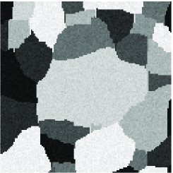
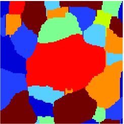
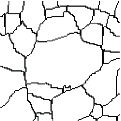
$f({\mathb{r}})$	$z({\mathb{r}})$	$c({\mathb{r}})$

Figure 1: Mod le de m lange et champs de Markov cach : image des intensit s ou niveau de gris $f({\mathb{r}})$, image $z({\mathb{r}})$ de segmentation ou classification, image binaire $c({\mathb{r}})$ des contours.

Ces diff rents cas peuvent alors se r sumer par :

Mod le de m lange s parables de gaussiennes (MSG):
C’est le mod le le plus simple o aucune structure spatiale n’est pris en compte a priori . Les relations qui donnent la loi a priori conjointe de $p({\mathb{f}},{\mathb{z}})=p({\mathb{f}}|{\mathb{z}})\;p({\mathb{z}})$ sont :

$$\left\{\begin{array}[]{lcl}p(f({\mathb{r}})|z({\mathb{r}})=k)&=&{\mathcal{N}}(m_{k},v_{k}),\forall{\mathb{r}}\in{\mathcal{R}}\\ p({\mathb{f}}|{\mathb{z}})&=&\prod_{{\mathb{r}}\in{\mathcal{R}}}{\mathcal{N}}(m_{z}({\mathb{r}}),v_{z}({\mathb{r}}))\end{array}\right.$$ (59)

avec $m_{z}({\mathb{r}})=m_{k},\forall{\mathb{r}}\in{\mathcal{R}}_{k}$ et $v_{z}({\mathb{r}})=v_{k},\forall{\mathb{r}}\in{\mathcal{R}}_{k}$, et

$$\left\{\begin{array}[]{lcl}p(z({\mathb{r}})=k)&=&\alpha_{k},\;\forall{\mathb{r}}\in{\mathcal{R}}\\ p({\mathb{z}})&=&\prod_{{\mathb{r}}}p(z({\mathb{r}})=k)=\prod_{k}\alpha_{k}^{n_{k}}\end{array}\right.$$ (60)

avec $n_{k}=\sum_{{\mathb{r}}\in{\mathcal{R}}}\delta(z({\mathb{r}})-k)$ le nombre de pixels dans la classe $k$ et $\sum_{k}n_{k}=n$ le nombre total des pixels de l’image. Les param tres de ce mod le sont

$${\boldsymbol{\theta}}_{f}=\{(\alpha_{k},m_{k},v_{k}),k=1,\cdots,K\}.$$

Rappelons aussi que $\sum_{k}\alpha_{k}=1$. Lors d’une estimation bay sienne non supervis e, il faut aussi attribuer des lois a priori ces param tres. les lois conjugu es correspondantes sont des gaussiennes pour $m_{k}$, des Inverse Gammas pour $v_{k}$ et la loi Dirichlet pour ${\boldsymbol{\alpha}}=[\alpha_{k},k=1,\cdots,K]$ :

$$\left\{\begin{array}[]{lcl}p(m_{k}|m_{0},v_{0})&=&{\mathcal{N}}(m_{0},v_{0}),\;\forall k\\ p(v_{k}|\alpha_{0},\beta_{0})&=&{\mathcal{I}}{\mathcal{G}}(a_{0},b_{0}),\;\forall k\\ p({\boldsymbol{\alpha}}|\alpha_{0})&=&{\mathcal{D}}(\alpha_{0}{\bf 1}_{K})\end{array}\right.$$ (61)

o $m_{0},v_{0},a_{0},b_{0}$ et $\alpha_{0}$ sont fix s pour un probl me donn e. On les choisis de telle sorte que ces lois soient les moins informatives (par exemple, $m_{0}=0$, $v_{0}=10$, $a_{0}=1$, $b_{0}=100$ et $\alpha_{0}=1/K$).

Mod le de m lange s parable de Gauss-Markov (MSGM):
Ici, la structure spatiale est pris en compte au travers d’un mod le markovien sur ${\mathb{f}}$ :

$$p(f({\mathb{r}})|z({\mathb{r}}),f({\mathb{r}}^{\prime}),z({\mathb{r}}^{\prime}),{\mathb{r}}^{\prime}\in{\mathcal{V}}({\mathb{r}}))={\mathcal{N}}(m_{z}({\mathb{r}}),v_{z}({\mathb{r}}))$$ (62)

avec

$$\begin{array}[]{lcl}m_{z}({\mathb{r}})&=&\frac{1}{|{\mathcal{V}}({\mathb{r}})|}\sum_{{\mathb{r}}^{\prime}\in{\mathcal{V}}({\mathb{r}})}m_{z({\mathb{r}}^{\prime})}^{*}\\ m_{z({\mathb{r}}^{\prime})}^{*}&=&\left\{\begin{array}[]{lll}\mu_{z({\mathb{r}}^{\prime})}&\mbox{si}&z({\mathb{r}}^{\prime})\not=z({\mathb{r}})\\ f({\mathb{r}}^{\prime})&\mbox{si}&z({\mathb{r}}^{\prime})=z({\mathb{r}})\end{array}\right.\end{array}$$ (63)

Par contre le champs ${\mathb{z}}$ est suppos s parable comme dans le premier cas (60).

On remarque que ${\mathb{f}}|{\mathb{z}}$ est un champ de Gauss-Markov non homog ne car la moyenne $m_{z}({\mathb{r}})$ et la variance $v_{z}({\mathb{r}})$ varient en fonction de ${\mathb{r}}$. Tous les pixels ${\mathb{f}}_{k}=\{f({\mathb{r}}),{\mathb{r}}\in{\mathcal{R}}_{k}\}$ se trouvant dans une r gion $k$ forment alors un vecteur gaussien de moyen $m_{k}{\bf 1}_{k}$ et de matrice de covariance ${\boldsymbol{\Sigma}}_{k}$ :

$$p({\mathb{f}}_{k})={\mathcal{N}}(m_{k}{\bf 1}_{k},v_{k}{\boldsymbol{\Sigma}}_{k})$$ (64)

o $v_{k}{\boldsymbol{\Sigma}}_{k}$ est une matrice de covariance de dimension $n_{k}\times n_{k}$ et ${\bf 1}_{k}=1$ est un vecteur de taille $n_{k}$ remplis de 1. Par ailleurs, on a aussi :

$$p({\mathb{f}}|{\mathb{z}})\propto\prod_{k}{\mathcal{N}}(m_{k}{\bf 1}_{k},v_{k}{\boldsymbol{\Sigma}}_{k})$$ (65)

ce qui signifie que les pixels appartenant aux diff rentes r gions sont ind pendantes.

Mod le de Gauss-Potts (MGP) :
Dans ce mod le, la structure spatiale est pris en compte au travers du mod le markovien de Potts (57) ou (58). La loi de $p({\mathb{f}}|{\mathb{z}})$ est la m me que dans le premier cas. En r sum , ici on a :

$$\left\{\begin{array}[]{lcl}p({\mathb{f}}|{\mathb{z}})&=&\prod_{{\mathb{r}}\in{\mathcal{R}}}{\mathcal{N}}(m({\mathb{r}}),v({\mathb{r}}))\\ p({\mathb{z}})&\propto&\exp\left[{\gamma\sum_{{\mathb{r}}\in{\mathcal{R}}}\sum_{{\mathb{r}}^{\prime}\in{\mathcal{V}}({\mathb{r}})}\delta(z({\mathb{r}})-z({\mathb{r}}^{\prime}))}\right]\end{array}\right.$$ (66)

avec $m({\mathb{r}})=m_{k},\forall{\mathb{r}}\in{\mathcal{R}}_{k}$ et $v({\mathb{r}})=v_{k},\forall{\mathb{r}}\in{\mathcal{R}}_{k}$.

Ici, donc, les pixels de l’images sont ind pendantes conditionnellement la connaissance des variables cach es, et donc, contrairement au cas pr c dent (64), ici on a $p({\mathb{f}}_{k})={\mathcal{N}}(m_{k}{\bf 1}_{k},v_{k}{\mathb{I}}_{k})$ o $v_{k}{\mathb{I}}_{k}$ est une matrice de covariance identit de dimension $n_{k}\times n_{k}$, ce qui permet d’ crire :

$$p({\mathb{f}}_{k})={\mathcal{N}}(m_{k}{\bf 1}_{k},v_{k}{\mathb{I}}_{k})\propto\exp\left[{\frac{-1}{2}\sum_{{\mathb{r}}\in{\mathcal{R}}_{k}}\frac{f({\mathb{r}})-m_{k})^{2}}{v_{k}}}\right]$$ (67)

et

$$p({\mathb{f}}|{\mathb{z}}) \propto \prod_{k}{\mathcal{N}}(m_{k}{\bf 1}_{k},{\mathb{I}}_{k})$$ (68)

$$\propto \exp\left[{\frac{-1}{2}\sum_{k}\sum_{{\mathb{r}}\in{\mathcal{R}}_{k}}\frac{(f({\mathb{r}})-m_{k})^{2}}{v_{k}}}\right]$$

ce qui signifie que, comme le cas pr c dent, les pixels appartenant aux diff rentes r gions sont ind pendantes.

Les param tres de ce mod le sont ${\boldsymbol{\theta}}_{f}=\{(\alpha_{k},m_{k},v_{k}),k=1,\cdots,K\}$ et $\gamma$. Malheureusement, il n’y a pas de loi conjugu e pour ce param tre et donc son estimation devient plus difficile. Dans ce travail, nous fixons ce param tre a priori .

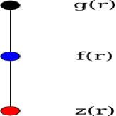
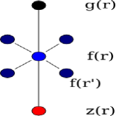
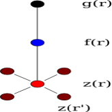
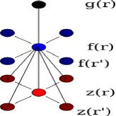
MSG	MSGM	MGP	MGMP

Figure 2: Quatre mod les de m lange avec champs cach s. Dans le mod le MSG toutes les variables sont s parables en ${\mathb{r}}$. Dans MSGM, $f({\mathb{r}})$ d pends de $z({\mathb{r}})$ et de ses voisins $f({\mathb{r}}^{\prime})$. Dans MGP, $z({\mathb{r}})$ d pends de ses voisin $z({\mathb{r}}^{\prime})$. Dans MGMP, $z({\mathb{r}})$ d pends de ses voisin $z({\mathb{r}}^{\prime})$ et $f({\mathb{r}})$ d pends de $z({\mathb{r}})$, $z({\mathb{r}}^{\prime})$ et de ses voisins $f({\mathb{r}}^{\prime})$.

Mod le de Gauss-Markov-Potts (MGMP) :
Il s’agit l de la composition des deux derniers mod les. Ici, nous r sumons ses relations d’une mani re l g rement diff rente en utilisant :

$$c_{{\mathb{r}}}({\mathb{r}}^{\prime})=1-\delta(z({\mathb{r}}^{\prime})-z({\mathb{r}}))=\left\{\begin{array}[]{lll}1&\mbox{si}&z({\mathb{r}}^{\prime})\not=z({\mathb{r}})\\ 0&\mbox{si}&z({\mathb{r}}^{\prime})=z({\mathb{r}})\end{array}\right.$$ (69)

ce qui donne :

$$p(f({\mathb{r}})|z({\mathb{r}}),f({\mathb{r}}^{\prime}),z({\mathb{r}}^{\prime}),{\mathb{r}}^{\prime}\in{\mathcal{V}}({\mathb{r}}))={\mathcal{N}}(m_{z}({\mathb{r}}),v_{z}({\mathb{r}}))$$ (70)

avec

$$m_{z}({\mathb{r}})=\frac{1}{|{\mathcal{V}}({\mathb{r}})|}\sum_{{\mathb{r}}^{\prime}\in{\mathcal{V}}({\mathb{r}})}\left[(1-c_{{\mathb{r}}}({\mathb{r}}^{\prime}))\mu_{z({\mathb{r}}^{\prime})}+c_{{\mathb{r}}}({\mathb{r}}^{\prime})f({\mathb{r}}^{\prime})\right]$$ (71)

et

$$p({\mathb{z}})\propto\exp\left[{\gamma\sum_{{\mathb{r}}\in{\mathcal{R}}}\sum_{{\mathb{r}}^{\prime}\in{\mathcal{V}}({\mathb{r}})}(1-c_{{\mathb{r}}}({\mathb{r}}^{\prime}))}\right]$$ (72)

En tous cas, quelque soit le mod le choisi parmi ces diff rents mod les, l’objectif est d’estimer ${\mathb{f}}$, ${\mathb{z}}$ et ${\boldsymbol{\theta}}$ en utilisant la loi a posteriori jointe :

$$p({\mathb{f}},{\mathb{z}},{\boldsymbol{\theta}}|{\mathb{g}})=\frac{p({\mathb{g}}|{\mathb{f}},{\boldsymbol{\theta}})\;p({\mathb{f}}|{\mathb{z}},{\boldsymbol{\theta}})\;p({\mathb{z}})}{p({\mathb{g}}|{\boldsymbol{\theta}})}$$ (73)

Bien que nous connaissons les expressions de tous les composants de num rateur de la fraction la droite de cette relation, le calcul du d nominateur n’est que rarement possible d’une mani re analytique. On cherche alors approcher $p({\mathb{f}},{\mathb{z}},{\boldsymbol{\theta}}|{\mathb{g}})$ par un produit des lois plus simples manipuler. Un premier choix est de l’approcher par une loi s parable $q({\mathb{f}},{\mathb{z}},{\boldsymbol{\theta}}|{\mathb{g}})=q_{1}({\mathb{f}})\;q_{2}({\mathb{z}})\;q_{3}({\boldsymbol{\theta}})$. Un deuxi me choix est $q_{1}({\mathb{f}}|{\mathb{z}})\;q_{2}({\mathb{z}})\;q_{3}({\boldsymbol{\theta}})$ qui permet de garder des liens forts qui existent entre ${\mathb{f}}$ et ${\mathb{z}}$ et de ne relaxer que des liens faibles entre ${\boldsymbol{\theta}}$ et ces deux derniers.

Le choix des familles appropri es pour $q_{1}({\mathb{f}}|{\mathb{z}})$ et $q_{2}({\mathb{z}})$ et $q_{3}({\boldsymbol{\theta}})$ pour chacun de ces mod les, qui est en lien avec les formes des lois a priori dans chacun de ces cas, et les expressions de la mise jour de ces diff rentes lois au cours des it rations n cessite beaucoup d’espace. Ici, nous allons juste fournir le principe et un r sum de ces relations.

Le choix de $q_{3}({\boldsymbol{\theta}})$, ou plus exactement, des familles des lois pour chacune des composentes de ${\boldsymbol{\theta}}$, qui sont la m me pour tous les cas, sont des lois conjugu es de (61). Par la suite, nous d taillons les choix de $q({\mathb{f}}|{\mathb{z}})$ et $q({\mathb{z}})$ dans les diff rent cas.

Cas 1 (MSG) :
Dans le cas du premier mod le on a

$$\left\{\begin{array}[]{lll}p({\mathb{f}}|{\mathb{z}})&=&\prod_{{\mathb{r}}}p(f({\mathb{r}})|z({\mathb{r}}))\\ p({\mathb{z}})&=&\prod_{{\mathb{r}}}p(z({\mathb{r}}))\end{array}\right.$$ (74)

o $p(f({\mathb{r}})|z({\mathb{r}})=k)={\mathcal{N}}(m_{k},v_{k})$ et $p(z({\mathb{r}})=k)=\alpha_{k}$, ce qui naturellement nous conduit choisir

$$\left\{\begin{array}[]{lll}q({\mathb{f}}|{\mathb{z}})&=&\prod_{{\mathb{r}}}q(f({\mathb{r}})|z({\mathb{r}}))\\ q({\mathb{z}})&=&\prod_{{\mathb{r}}}q(z({\mathb{r}}))\end{array}\right.$$ (75)

avec $q(f({\mathb{r}})|z({\mathb{r}})=k)={\mathcal{N}}(\tilde{m}_{k},\tilde{v}_{k})$ et $q(z({\mathb{r}})=k)=\tilde{\alpha}_{k}$.

Au cours des it rations, $\tilde{m}_{k}$ $\tilde{v}_{k}$ et $\tilde{\alpha}_{k}$ seront mise jour.

Cas 2 (MSGM) :
Dans le deuxi me cas, le mod le de m lange de Gauss-Markov, notant que

$$p({\mathb{f}}|{\mathb{z}})=\prod_{{\mathb{r}}}{\mathcal{N}}(f({\mathb{r}})|m_{z}({\mathb{r}}),v_{z}({\mathb{r}}))$$ (76)

o

$$m_{z}({\mathb{r}})=\frac{1}{|{\mathcal{V}}({\mathb{r}})|}\sum_{{\mathb{r}}^{\prime}\in{\mathcal{V}}({\mathb{r}})}m_{z({\mathb{r}}^{\prime})}^{*}$$ (77)

avec

$$m_{z({\mathb{r}}^{\prime})}^{*}=\delta(z({\mathb{r}}^{\prime})-z({\mathb{r}}))f({\mathb{r}}^{\prime})+(1-\delta(z({\mathb{r}}^{\prime})-z({\mathb{r}}))\mu_{z({\mathb{r}}^{\prime})}$$ (78)

on trouve naturellement l’approximation suivante :

$$m_{z({\mathb{r}}^{\prime})}^{*}=\delta(z({\mathb{r}}^{\prime})-z({\mathb{r}}))\tilde{f}({\mathb{r}}^{\prime})+(1-\delta(z({\mathb{r}}^{\prime})-z({\mathb{r}}))\tilde{m}_{z({\mathb{r}})}$$ (79)

o $\tilde{f}({\mathb{r}}^{\prime})$ est l’esp rance de $f({\mathb{r}}^{\prime})$ calcul e l’ tape pr c dente. Il s’agit de l’approximation dite en champs moyens pour le champ de Markov ${\mathb{f}}$ :

$$\left\{\begin{array}[]{@{}l@{}l@{}l@{}}q({\mathb{f}}|{\mathb{z}})&=&\prod_{{\mathb{r}}}q(f({\mathb{r}})|z({\mathb{r}}))=\prod_{{\mathb{r}}}{\mathcal{N}}(f({\mathb{r}})|m_{z}({\mathb{r}}),v_{z}({\mathb{r}}))\\ \mbox{avec}\\ m_{z}({\mathb{r}})&=&\frac{1}{|{\mathcal{V}}({\mathb{r}})|}\sum_{{\mathb{r}}^{\prime}\in{\mathcal{V}}({\mathb{r}})}\\ &&\delta(z({\mathb{r}})-z({\mathb{r}}^{\prime}))f({\mathb{r}})+(1-\delta(z({\mathb{r}})-z({\mathb{r}}^{\prime})))\mu_{z({\mathb{r}})}\end{array}\right.$$ (80)

Cas 3 (MGP) :
Dans le troisi me cas, le mod le de Gauss-Potts on a

$$\left\{\begin{array}[]{lll}p({\mathb{f}}|{\mathb{z}})&=&\prod_{{\mathb{r}}}p(f({\mathb{r}})|z({\mathb{r}}))\\ p({\mathb{z}})&=&\prod_{{\mathb{r}}}p(z({\mathb{r}})|z({\mathb{r}}^{\prime}),{\mathb{r}}^{\prime}\in{\mathcal{V}}({\mathb{r}}))\end{array}\right.$$ (81)

ce qui naturellement nous conduit choisir

$$\left\{\begin{array}[]{lll}q({\mathb{f}}|{\mathb{z}})&=&\prod_{{\mathb{r}}}q(f({\mathb{r}})|z({\mathb{r}}))\\ q({\mathb{z}})&=&\prod_{{\mathb{r}}}q(z({\mathb{r}})|\bar{z}({\mathb{r}}^{\prime}),{\mathb{r}}^{\prime}\in{\mathcal{V}}({\mathb{r}}))\end{array}\right.$$ (82)

o nous avons choisi une approximation en champs moyens pour le champs de Potts. Cette approximation suppl mentaire qui consiste remplacer les valeurs de $z({\mathb{r}}^{\prime})$ par leurs moyenne $\bar{z}({\mathb{r}}^{\prime})$ est une approximation courante pour un mod le de Potts.

Cas 4 (MGMP) :
Dans le quatri me cas,le Mod le de Gauss-Markov-Potts on a

$$\left\{\begin{array}[]{@{}l@{}l@{}l@{}}q({\mathb{f}}|{\mathb{z}})&=&\prod_{{\mathb{r}}}q(f({\mathb{r}})|z({\mathb{r}}))=\prod_{{\mathb{r}}}{\mathcal{N}}(f({\mathb{r}})|m_{z}({\mathb{r}}),v_{z}({\mathb{r}}))\\ \mbox{avec}\\ m_{z}({\mathb{r}})&=&\frac{1}{|{\mathcal{V}}({\mathb{r}})|}\sum_{{\mathb{r}}^{\prime}\in{\mathcal{V}}({\mathb{r}})}\\ &&\delta(z({\mathb{r}})-z({\mathb{r}}^{\prime})f({\mathb{r}})+(1-\delta(z({\mathb{r}})-z({\mathb{r}}^{\prime}))\mu_{z({\mathb{r}})}\\ q({\mathb{z}})&=&\prod_{{\mathb{r}}}q(z({\mathb{r}})|\bar{z}({\mathb{r}}^{\prime}),{\mathb{r}}^{\prime}\in{\mathcal{V}}({\mathb{r}}))\end{array}\right.$$ (83)

Dans tous les cas, puisque les lois a priori pour les diff rent composants de ${\boldsymbol{\theta}}=\{\{\theta_{e_{i}}\},\{m_{k}\},\{v_{k}\},\{\beta_{k}\}\}$ sont des lois conjugu es et s parables, on choisi

$$q({\boldsymbol{\theta}})=\prod_{i}q(\theta_{i})$$ (84)

Il reste un param tre que nous garderons fixe. C’est le param tre du mod le de Potts. En effet, n’ayant pas une expression analytique pour la fonction de r partition du mod le de Potts, il n’existe pas une loi conjugu e pour ce param tre. Dans un premier temps donc, nous gardons ce param tre comme un param tre de r glage non supervis .

Les deux tableaux qui suivent r sument les lois a priori et les choix des lois s parables pour les quatre cas propos s.

Mod le	MSG	MSGM	MGP	MGMP
$p({\mathb{f}}|{\mathb{z}})$	$\displaystyle{\prod_{{\mathb{r}}}{\mathcal{N}}(m_{z}({\mathb{r}}),v_{z}({\mathb{r}}))}$	Gauss-Markov	$\displaystyle{\prod_{{\mathb{r}}}{\mathcal{N}}(m_{z}({\mathb{r}}),v_{z}({\mathb{r}}))}$	Gauss-Markov
$p({\mathb{z}})$	$\displaystyle{\prod_{{\mathb{r}}}\alpha_{z}({\mathb{r}})=\prod_{k}\alpha_{k}^{n_{k}}}$	$\displaystyle{\prod_{{\mathb{r}}}\alpha_{z}({\mathb{r}})=\prod_{k}\alpha_{k}^{n_{k}}}$	Potts	Potts
$p(m_{k})$	${\mathcal{N}}(m_{0},v_{0})$	${\mathcal{N}}(m_{0},v_{0})$	${\mathcal{N}}(m_{0},v_{0})$	${\mathcal{N}}(m_{0},v_{0})$
$p(v_{k})$	${\mathcal{I}}{\mathcal{G}}(a_{0},b_{0})$	${\mathcal{I}}{\mathcal{G}}(a_{0},b_{0})$	${\mathcal{I}}{\mathcal{G}}(a_{0},b_{0})$	${\mathcal{I}}{\mathcal{G}}(a_{0},b_{0})$
$p({\boldsymbol{\alpha}})$	${\mathcal{D}}(\alpha_{0},\cdots,\alpha_{0})$	${\mathcal{D}}(\alpha_{0},\cdots,\alpha_{0})$	${\mathcal{D}}(\alpha_{0},\cdots,\alpha_{0})$	${\mathcal{D}}(\alpha_{0},\cdots,\alpha_{0})$
$p(\theta_{e})$	${\mathcal{G}}(a_{\epsilon_{0}},b_{\epsilon_{0}})$	${\mathcal{G}}(a_{\epsilon_{0}},b_{\epsilon_{0}})$	${\mathcal{G}}(a_{\epsilon_{0}},b_{\epsilon_{0}})$	${\mathcal{G}}(a_{\epsilon_{0}},b_{\epsilon_{0}})$
$q({\mathb{f}}|{\mathb{z}})$	$\displaystyle{\prod_{{\mathb{r}}}{\mathcal{N}}(\hat{\mu}_{z}({\mathb{r}}),\hat{v}_{z}({\mathb{r}}))}$	$\displaystyle{\prod_{{\mathb{r}}}{\mathcal{N}}(\hat{\mu}_{z}({\mathb{r}}),\hat{v}_{z}({\mathb{r}}))}$	$\displaystyle{\prod_{{\mathb{r}}}{\mathcal{N}}(m_{z}({\mathb{r}}),v_{z}({\mathb{r}}))}$	$\displaystyle{\prod_{{\mathb{r}}}{\mathcal{N}}(\hat{\mu}_{z}({\mathb{r}}),\hat{v}_{z}({\mathb{r}}))}$
$q({\mathb{z}})$	$\displaystyle{\prod_{{\mathb{r}}}\hat{\alpha}_{z}({\mathb{r}})=\prod_{k}\hat{\alpha}_{k}^{n_{k}}}$	$\displaystyle{\prod_{{\mathb{r}}}\hat{\alpha}_{z}({\mathb{r}})=\prod_{k}\hat{\alpha}_{k}^{n_{k}}}$	$\displaystyle{\prod_{{\mathb{r}}}q(z({\mathb{r}})|\bar{z}({\mathb{r}}^{\prime}),{\mathb{r}}^{\prime}\in{\mathcal{V}}({\mathb{r}}))}$	$\displaystyle{\prod_{{\mathb{r}}}q(z({\mathb{r}})|\bar{z}({\mathb{r}}^{\prime}),{\mathb{r}}^{\prime}\in{\mathcal{V}}({\mathb{r}}))}$
$q(m_{k})$	${\mathcal{N}}(\hat{m}_{k},\hat{v}_{k})$	${\mathcal{N}}(\hat{m}_{k},\hat{v}_{k})$	${\mathcal{N}}(\hat{m}_{k},\hat{v}_{k})$	${\mathcal{N}}(\hat{m}_{k},\hat{v}_{k})$
$q(v_{k})$	${\mathcal{I}}{\mathcal{G}}(\hat{a}_{k},\hat{b}_{k})$	${\mathcal{I}}{\mathcal{G}}(\hat{a}_{k},\hat{b}_{k})$	${\mathcal{I}}{\mathcal{G}}(\hat{a}_{k},\hat{b}_{k})$	${\mathcal{I}}{\mathcal{G}}(\hat{a}_{k},\hat{b}_{k})$
$q({\boldsymbol{\alpha}})$	${\mathcal{D}}(\hat{\alpha}_{1},\cdots,\hat{\alpha}_{K})$	${\mathcal{D}}(\hat{\alpha}_{1},\cdots,\hat{\alpha}_{K})$	${\mathcal{D}}(\hat{\alpha}_{1},\cdots,\hat{\alpha}_{K})$	${\mathcal{D}}(\hat{\alpha}_{1},\cdots,\hat{\alpha}_{K})$
$q(\theta_{e})$	${\mathcal{G}}(\hat{a}_{\epsilon_{0}},\hat{b}_{\epsilon_{0}})$	${\mathcal{G}}(\hat{a}_{\epsilon_{0}},\hat{b}_{\epsilon_{0}})$	${\mathcal{G}}(\hat{a}_{\epsilon_{0}},\hat{b}_{\epsilon_{0}})$	${\mathcal{G}}(\hat{a}_{\epsilon_{0}},\hat{b}_{\epsilon_{0}})$

Table 1: Les lois a priori et les lois s parables approchantes pour les quatre mod les propos s.

Ici, nous ne d veloppons pas plus les expressions de la mise jour de ces diff rentes loi au cours des it rations, mais ce qu’il faut savoir est que toutes ces lois tant de formes param triques connues (gaussienne, gamma ou inverse gamma, Wishart ou inverse Wishart et Dirichlet), nous avons des expressions analytiques pour les esp rances de ces lois. Les d tails de ces relations accompagn s des r sultats de simulation seront communiqu s dans un autre papier dans un future proche.

6 R sultats et discussions

Nous avons utilis cette approche dans plusieur domaines de probl mes inverses : i) restauration d’image [53, 42], ii) reconstruction d’image en tomographie X [54, 55], et iii) s paration de sources et segmentation des images hyperspectrales [40]. Nous sommes aussi en train de mettre en oeuvre ces algorithmes pour le cas 3D de la tomographie X ainsi qu’au cas de l’imagerie microondes.

Dans tous ces applications, nous avons impl ment la fois des algorithmes MCMC ( chantillonneurs de Gibbs) et l’approche variationnelle bay sienne (VB) d velopp e dans cet article. Nous avons ainsi pu compar les r sultats obtenus par ces deux m thodes. D’une mani re g n rale, les principales conclusions de ces exp rimentations et comparaisons sont : i) la qualit des r sultats obtenus sont pratiquement similaires, et ii) le principal avantage de l’approche VB est dans le gain en temps de calcul qui d pend bien sure du contexte et de l’applications.

Un autre avantage important que l’on peut mentionner est l’existance d’un crit re (l’ nergie libre, quation 10) que l’on peut utiliser : i) comme crit re d’arr t pour l’algorithme et ii) comme un crit re de choix de mod le. En effet, comme nous l’avons vu, gr ce la relation 9, minimiser $\mbox{KL}(q:p)$ est quivalent maximiser ${\mathcal{F}}(q)$ et sa valeur optimale est un bon indicateur pour $\ln p({\mathb{g}}|{\mathcal{M}})$. Ainsi, les valeurs relatives de ${\mathcal{F}}(q)$ au cours des it rations de l’algorithme peuvent tre utilis es comme un crit re d’arr t et sa valeur optimale atteint pour un mod le ${\mathcal{M}}_{1}$ peut tre compar e sa valeur optimale atteint pour un autre mod le ${\mathcal{M}}_{2}$ comme un crit re de pr f rence entre les deux mod les.

7 Conclusion

L’approche variationnelle de l’approximation d’une loi par des lois s parables est appliqu e au cas de l’estimation non supervis e des inconnues et des hyperparam tres dans des probl mes inverses de restauration d’image (d convolution simple ou aveugle) avec des mod lisations a priori gaussiennes, gaussiennes g n ralis es, m lange de gaussiennes ind pendantes ou m lange de Gauss-Markov avec champs cach s des tiquettes ind pendantes ou markovien (Potts).

Dans ce papier, nous avons d crit d’abord le principe de l’approximation d’une loi et ensuite propos des approximations appropri es pour des lois a posteriori conjointes que l’on trouve dans le cas des probl mes inverses en g n ral et en restauration d’images en particulier. Cependant, la mise en oeuvre effective de ces m thodes est en cours et les r sultats de simulation et valuation des performances de ces m thodes seront communiqu s dans un future proche.

Les d tails de ces relations accompagn s des r sultats de simulation qui sont disponible sous forme d’un rapport [53, 42] seront communiqu s dans un autre papier en pr paration dans un futur proche.

8 Remerciment

L’author souhaite remercier Jean-Fran ois Berchet et Guy Demoment pour les discussions fructueuses et la relecture de la premi re version de ce papier, H. Ayasso et S. Fekih pour l’impl mentation de ces algorithmes en restauration d’image et en tomographie X, N. Bali pour l’impl mentation de ces algorithmes en s paration de sources et en imagerie hyperspectrale.

• [1] J. Rustagi, Variational methods in statistics. New York: Academic Press, 1976.
• [2] Z. Ghahramani and M. Jordan, “Factorial Hidden Markov Models,” Machine Learning, no. 29, pp. 245–273, 1997.
• [3] W. Penny and S. Roberts, “Bayesian neural networks for classification: how useful is the evidence framework ?,” Neural Networks, vol. 12, pp. 877–892, 1998.
• [4] S. Roberts, D. Husmeier, W. Penny, and I. Rezek, “Bayesian approaches to gaussian mixture modelling,” IEEE Transactions on Pattern Analysis and Machine Intelligence, vol. 20, no. 11, pp. 1133–1142, 1998.
• [5] H. Attias, “Independent factor analysis,” Neural Computation, vol. 11, no. 4, pp. 803–851, 1999.
• [6] M. Jordan, Z. Ghahramani, T. Jaakkola, , and L. Saul, “An introduction to variational methods for graphical models,” Machine Learning, vol. 37, pp. 183–233, 2006.
• [7] W. Penny and S. Roberts, “Dynamic models for nonstationary signal segmentation,” Computers and Biomedical Research, vol. 32, no. 6, pp. 483–502, 1999.
• [8] H. Attias, “A variational Bayesian framework for graphical models.,” in Advances in Neural Information Processing Systems (S. Solla, T. K. Leen, and K. L. Muller, eds.), vol. 12, pp. 209–215, MIT Press, 2000.
• [9] T. Jaakkola, “Tutorial on variational approximation methods,” in Advanced mean field methods: theory and practice. (M. Opper and D. Saad, eds.), (Cambridge, Massachusetts), pp. 129–159, 2000.
• [10] J. Miskin, Ensemble Learning for Independent Component Analysis. Thèse de doctorat, Cambridge, 2000, http://www.inference.phy.cam.ac.uk/jwm1003/.
• [11] J. W. Miskin and D. J. C. MacKay, “Application of ensemble learning to infra-red imaging,” in Proceedings of the Second International Workshop on Independent Component Analysis and Blind Signal Separation, pp. 399–404, 2000.
• [12] J. W. Miskin and D. J. C. MacKay, “Ensemble learning for blind source separation,” in ICA: Principles and Practice (S. Roberts and R. Everson, eds.), Cambridge: Cambridge University Press, 2001.
• [13] W. Penny and S. Roberts, “Bayesian multivariate autoregresive models with structured priors,” IEE Proceedings on Vision, Image and Signal Processing, vol. 149, no. 1, pp. 33–41, 2002.
• [14] S. Roberts and W. Penny, “Variational bayes for generalised autoregressive models,” IEEE Transactions on Signal Processing, vol. 50, no. 9, pp. 2245–2257, 2002.
• [15] M. Cassidy and W. Penny, “Bayesian nonstationary autogregressive models for biomedical signal analysis,” IEEE Transactions on Biomedical Engineering, vol. 49, no. 10, pp. 1142–1152, 2002.
• [16] W. Penny and K. Friston, “Mixtures of general linear models for functional neuroimaging,” IEEE Transactions on Medical Imaging, vol. 22, no. 4, pp. 504–514, 2003.
• [17] W. Penny, S. Kiebel, and K. Friston, “Variational Bayesian inference for fmri time series,” NeuroImage, vol. 19, no. 3, pp. 727–741, 2003.
• [18] R. A. Choudrey and S. Roberts, “Variational bayesian mixture of independent component analysers for finding self-similar areas in images,” in Proc. 4th International Symposium on Independent Component Analysis and Blind Signal Separation (ICA2003), (Nara, Japan), pp. 107–112, April 2003.
• [19] R. Choudrey and S. Roberts, “Variational Mixture of Bayesian Independent Component Analysers,” Neural Computation, vol. 15, no. 1, 2003.
• [20] W. Penny, R. Everson, and S. Roberts, “Hidden markov independent component analysis,” in Advances in Independent Component Analysis (M. Giroliami, ed.), Springer, 2000.
• [21] D. M. Blei and M. I. Jordan, “Variational methods for the dirichlet process,” in ICML, 2004.
• [22] N. Nasios and A. Bors, “A variational approach for Bayesian blind image deconvolution,” IEEE Transactions on Signal Processing, vol. 52, no. 8, pp. 2222–2233, 2004.
• [23] C. Archambeau, T. Butz, V. Popovici, M. Verleysen, and J. Thiran, “Supervised nonparametric information theoretic classification,” in Proceedings of the 17th International Conference on Pattern Recognition, vol. 3, pp. 414–417, IEEE, August 2004.
• [24] M. Woolrich, E. Timothy, F. Christian, and S. Smith, “Mixture models with adaptive spatial regularization for segmentation with an application to fmri data,” IEEE Trans. on Medical Imaging, vol. 24, pp. 1–11, January 2005.
• [25] D. M. Blei and M. I. Jordan, “Variational methods for the dirichlet process,” Journal Version (TODO: which?), 2006.
• [26] M. Beal and Z. Ghahramani, “Variational Bayesian learning of directed graphical models with hidden variables,” Bayesian Statistics, vol. 1, pp. 793–832, 2006.
• [27] H. Kim and Z. Ghahramani, “Bayesian gaussian process classification with the em-ep algorithm,” IEEE Transactions on Pattern Analysis and Machine Intelligence, vol. 28, no. 12, pp. 1948–1959, 2006.
• [28] B. Wang and D. Titterington, “Convergence properties of a general algorithm for calculating variational bayesian estimates for a normal mixture model,” Bayesian Analysis, vol. 1, pp. 625–650, 2006.
• [29] K. Watanabe and S. Watanabe, “Stochastic complexities of gaussian mixtures in variational bayesian approximation,” Journal of Machine Learning Research, pp. 625–644, April 2006.
• [30] N. Nasios and A. Bors, “Variational learning for gaussian mixture models,” IEEE Transactions on Systems, Man and Cybernetics, Part B, vol. 36, no. 4, pp. 849–862, 2006.
• [31] K. Friston, J. Mattout, N. Trujillo-Barreto, J. Ashburner, and W. Penny, “Variational free energy and the laplace approximation,” Neuroimage, no. 2006.08.035, 2006. Available Online.
• [32] W. Penny, S. Kiebel, and K. Friston, “Variational bayes,” in Statistical Parametric Mapping: The analysis of functional brain images (K. Friston, J. Ashburner, S. Kiebel, T. Nichols, and W. Penny, eds.), Elsevier, London, 2006.
• [33] Z. Ghahramani, T. Griffiths, and P. Sollich, “Bayesian nonparametric latent feature models,” Bayesian Statistics, vol. 8, 2007.
• [34] C. McGrory and D. Titterington, “Variational approximations in Bayesian model selection for finite mixture distributions,” Computational Statistics and Data Analysis, vol. 51, no. 11, pp. 5352–5367, 2007.
• [35] F. Forbes and F. Gersende, “Combining monte carlo and mean-field-like methods for inference in hidden markov random fields,” IEEE Trans. on Image Processing, vol. 16, pp. 824–835, March 2007.
• [36] M. Ichir and A. Mohammad-Djafari, “A mean field approximation approach to blind source separation with lp priors,” in Eusipco 2005, Antalya, Turkey, September 2005, Eusipco 2005, Antalya, Turkey, September 2005, September 2005.
• [37] M. Ichir and A. Mohammad-Djafari, “Hidden markov models for wavelet image separation and denoising,” in Proc. IEEE International Conference on Acoustics, Speech, and Signal Processing (ICASSP ’05), vol. 5, pp. v/225–v/228, 18–23 March 2005.
• [38] H. Snoussi and A. Mohammad-Djafari, “Estimation of structured gaussian mixtures: The inverse em algorithm,” IEEE Trans. on Signal Processing, vol. 55, pp. 3185–3191, July 2007.
• [39] N. Bali and A. Mohammad-Djafari, “Mean Field Approximation for BSS of images with compound hierarchical Gauss-Markov-Potts model,” in MaxEnt05,San José CA,US, American Institute of Physics (AIP), August 2005.
• [40] N. Bali and A. Mohammad-Djafari, “Bayesian approach with hidden markov modeling and mean field approximation for hyperspectral data analysis,” IEEE Trans. on Image Processing, vol. 17, pp. 217–225, Feb. 2008.
• [41] A. Mohammad-Djafari, “Approche variationnelle pour le calcul bayésien dans les problèmes inverses en imagerie,” in GRETSI, Troyes, France, September 2007.
• [42] H. Ayasso and A. Mohammad-Djafari, “Variational bayes with gauss-markov-potts prior models for joint image restoration and segmentation,” Visapp Proceedings, (Funchal, Madaira, Portugal), Int. Conf. on Computer Vision and Applications, 2008.
• [43] A. Mohammad-Djafari, “Gauss-markov-potts priors for images in computer tomography resulting to joint optimal reconstruction and segmentation,” International Journal of Tomography & Statistics, vol. 11, no. W09, pp. 76–92, 2008.
• [44] R. Molina, A. K. Katsaggelos, and J. Mateos, “Bayesian and regularization methods for hyperparameter estimation in image restoration,” IEEE Transactions on Image Processing, vol. 8, pp. 231–246, February 1999.
• [45] A. Likas and N. Galatsanos, “A variational approach for Bayesian blind image deconvolution,” IEEE Trans. on Signal Processing, vol. 52, pp. 2222–2233, August 2004.
• [46] K. Blekas, A. Likas, N. Galatsanos, and I. Lagaris, “A spatially-constrained mixture model for image segmentation,” IEEE Trans. on Signal Processing, vol. 16, pp. 494–498, March 2005.
• [47] A. Mohammad-Djafari and L. Robillard, “Hierarchical Markovian models for 3D computed tomography in non destructive testing applications,” in EUSIPCO 2006, EUSIPCO 2006, September 4-8, Florence, Italy, September 2006.
• [48] M. Patriksson, Nonlinear programming and variational inequality problems. A unified approach. Applied Optimization, Dordrecht, The Netherlands: Kluwer Academic Publishers, May 1999.
• [49] R. Choudrey, W. Penny, and S. Roberts, “An ensemble learning approach to independent component analysis,” in IEEE Workshop on Neural Networks for Signal Processing, Sydney Australia, 2000.
• [50] W. Penny and S. Roberts, “Variational bayes for non-gaussian autoregressive models,” in IEEE Workshop on Neural Networks for Signal Processing, Sydney Australia, 2000.
• [51] R. Choudrey and S. Roberts, “Variational Bayesian Mixture of Independent Component Analysers for Finding Self-Similar Areas in Images,” in ICA, NARA, JAPAN, April 2003.
• [52] B. R. Hunt, “A matrix theory proof of the discrete convolution theorem,” IEEE Transactions on Automatic and Control, vol. AC-19, pp. 285–288, 1971.
• [53] H. Ayasso and A. Mohammad-Djafari, “Approche bayésienne variationnelle pour les problèmes inverses. application en tomographie microonde,” tech. rep., Rapport de stage Master ATS, Univ Paris Sud, L2S, SUPELEC, 2007.
• [54] H. Ayasso, S. Fekih-Salem, and A. Mohammad-Djafari, “Variational bayes approach for tomographic reconstruction,” in Proceedings of the 28th International Workshop on Bayesian Inference and Maximum Entropy Methods in Science and Engineering, MaxEnt, vol. 1073, (Boraceia, Sao Paulo (Brazil)), pp. 243–251, AIP, November 2008.
• [55] H. Ayasso and A. Mohammad-Djafari, “Joint image restoration and segmentation using gauss-markov-potts prior models and variational bayesian computation,” Submitted to IEEE Image Processing, Febuary, 2009.