Edge disorder and localization regimes in bilayer graphene nanoribbons

Abstract

A theoretical study of the magnetoelectronic properties of zigzag and armchair bilayer graphene nanoribbons (BGNs) is presented. Using the recursive Green’s function method, we study the band structure of BGNs in uniform perpendicular magnetic fields and discuss the zero-temperature conductance for the corresponding clean systems. The conductance quantized as $2(n+1)G_{0}$ for the zigzag edges and $nG_{0}$ for the armchair edges with $G_{0}=2e^{2}/h$ being the conductance unit and $n$ an integer. Special attention is paid to the effects of edge disorder. As in the case of monolayer graphene nanoribbons (GNR), a small degree of edge disorder is already sufficient to induce a transport gap around the neutrality point. We further perform comparative studies of the transport gap $E_{g}$ and the localization length $\xi$ in bilayer and monolayer nanoribbons. While for the GNRs $E_{g}^{GNR}\sim 1/W$, the corresponding transport gap $E_{g}^{BGN}$ for the bilayer ribbons shows a more rapid decrease as the ribbon width $W$ is increased. We also demonstrate that the evolution of localization lengths with the Fermi energy shows two distinct regimes. Inside the transport gap, $\xi$ is essentially independent on energy and the states in the BGNs are significantly less localized than those in the corresponding GNRs. Outside the transport gap $\xi$ grows rapidly as the Fermi energy increases and becomes very similar for BGNs and GNRs.

I Introduction

The recent successful fabrication of monolayer graphene Novoselov has ignited tremendous interest because it not only represents a platform to model relativistic particles in a condensed matter material, but also provides a potential building block for future nanoelectronics. The honeycomb lattice of the graphene sheet imposes a linear low-energy electronic spectrum and the corresponding extraordinary electronic behavior of the excitations near the Dirac point, namely massless Dirac fermions Katsnelson ; Neto2009 . Various aspects of graphene like band structures Wakabayashi1999 ; Brey2006 and resulting transport properties Rojas2006 ; Lewenkopf2008 ; Chen2007 ; Han2007 ; Wang2008 have been studied. Electrostatic potentials Katsnelson and magnetic barriers Martino2007 ; Xu2008 ; Masir2008 have been suggested as ways to achieve tunable confinement. Moreover, there have been suggestions to induce a bandgap and manipulate efficiently the resistance by, for example, chemical doping Filho2007 , edge disorder Evaldsson2008 , while studies of the magnetoelectronic properties also revealed the anomalous integer and fractional quantum Hall effects in graphene Zhang2005 ; Novoselov2005 ; Gusynin2005 ; Peres2006 .

More recently, increasing attention has been paid to graphene multilayers, in particular to bilayer systems Mccann2006 ; Kechedzhi2007 ; Snyman2007 ; Abergel2007 ; Lai2008 which consist of two coupled graphene sheets with two sublattices, $A$ and $B$, in each layer. They are typically stacked in the Bernal form, where $A^{\prime}$ sites belonging to the upper layer are located exactly on the top of $B$ sites to the lower layer, and $B^{\prime}$ or $A$ sites are above or below the center of hexagons in the other layer, as shown in Fig. 1. Bilayers show quite different properties than monolayers in many respects, such as the quantum Hall effect Mccann2006 ; Novoselov2005 , edge states Castro2008 , and weak localization Gorbachev . Graphene bilayers are also inevitably influenced by the disorder present in the environment. The role of disorder in graphene bilayers has been studied theoretically Nilsson2008 and the minimal conductivity has been addressed by different authors Katsnelson2006 ; Cserti . An important property of graphene bilayers is that an application of an electric field between the layers allows to open up and tune a band gap, which is highly relevant for the possible applications in nanoelectronics. Experimentally, a double-gate configuration can impose a perpendicular electric field onto a bilayer, and a controlled transition from a zero-gap semiconductor to an insulator has been observed, which provides a direct evidence of opening a bias-induced band gap in a bilayer Oostinga . It has been shown that a bias voltage can continuously tune a bandgap from zero to mid-infrared frequencies around the zero-energy point Castro2007 , modify the charge density distribution in the graphene planes Mccannprb2006 and even induce the low-density ferromagnetism Castroprl2008 .

To study the properties of bulk bilayer graphene theoretically, the effective Dirac-like Hamiltonian as the continuum limit of the tight-binding model close to the Dirac points was mostly used. It has been applied to the study of the energy spectrum of bilayers Falko2009 , to the transport phenomenology through biased Nilsson2007 and unbiased Nilsson2006 graphene bilayers with bulk disorder as well as to the bilayer/monolayer interface Nilsson_prb_2007 . However, the energy spectra and the transport properties of bilayer graphene nanoribbons (BGNs), which form the focus of this paper, have not yet been addressed in the literature to the best of our knowledge.

The purpose of the present work is twofold. First, we develop a computational method and present a theoretical study of the magneto-band structure, Bloch states and conductance quantization in zigzag and armchair BGNs. Our method is based on the recursive Green’s function technique that we recently developed to calculate the electronic structure and conductance of graphene nanoribbons Xu2008 . The special feature of this technique is that, in contrast to earlier Green’s function methods, it does not require self-consistent calculations for the surface Green’s function, which is instead computed as a solution of an eigenequation. This greatly reduces the computation time. Making use of this technique, one can study the band structure and conductance of BGNs of various geometries and edge terminations in various transport scenarios including a perpendicular magnetic field, a bias voltage, etc. It should also be noted that the electron-electron interaction and screening can significantly affect and modify electronic properties of single-layer graphene nanoribbons Fernandez-Rossier ; Efetov . It is expected that screening in the BGNs differs from that one in GNRs, because the electrons in each layer are affected not only by the electrons belonging to the same layer, but also by the electrons in the second layer. A detailed knowledge of the electronic structure of an ideal BGNs (without interaction) is a prerequisite for any studies of interaction effects in this system. While accounting for electron interactions will be the subject of future studies, knowledge of electronic structure of the ideal BGN represents a necessary first step in this direction.

Second, the effects of edge disorder on the conductance of BGNs are investigated. It is well established that the edge disorder strongly affects the transport properties of monolayer graphene nanoribbons leading to the suppression of the conductance quantization and opening of the transport gap Chen2007 ; Han2007 ; Areshkin ; Louis ; Gunlycke ; Li ; Querlioz ; Avouris ; Evaldsson2008 ; Mucciolo . We are not aware of any work addressing the effect of edge disorder on the transport properties of BGNs and our study represents a first step in this direction. We demonstrate that conductance of realistic BGNs with edge disorder share many similar features with that one of the monolayer GNRs. There are however important and interesting differences that we discuss in detail.

The paper is organized as follows. In Section II, we sketch the geometry of the devices and the Green’s functions technique that we use. In Section III, we present the band structures and the conductance of ideal BGNs. Section IV focuses on the effects of edge disorder. A summary and conclusions constitute Section V.

Figure 1: (Color online) Schematic geometry of the two-terminal structure for the case of (a) zigzag and (b) armchair BGNs. The devices under consideration are indicated by the shaded regions which connect to the two semi-infinite leads opening to the left and right. Bonds in the bottom layer are indicated by dashed lines and in the top layer by solid lines. Empty and filled circles denote the atoms in the lower and upper layers, respectively. Unit cells of the BGNs are marked by bold dashed rectangles. Vertical dashed lines with numbers label the slices of a unit cell; the numbers with and without prime labels refer to respective upper and lower layers, for example, $1$ and $1^{\prime}$ correspond to the first slice. $a$ is the carbon-carbon bond length. Numbers in the vertical direction label the sites in a slice. (c) 3D view of the graphene bilayer with all coupling energies. Two interpenetrating triangular sublattices sublattices in the lower and upper layers are denoted $A$, $B$, and $A^{\prime}$, $B^{\prime}$, respectively. $\gamma_{0}$ is the coupling between nearest-neighboring sites in the same layer. Interlayer coupling energies include $\gamma_{1}$ between $A^{\prime}$ and $B$, $\gamma_{3}$ between $B^{\prime}$ and $A$, and $\gamma_{4}$ between $A^{\prime}(B^{\prime})$ and $A(B)$ ($\gamma_{4}$ is neglected in our calculations).

II Model descriptions

We shall consider the two-terminal BGN structure sketched in Fig. 1(a) and (b). The semi-infinite left and right leads are made of zigzag or armchair BGNs. In the shaded central region, one can define a structure of interest, such as an electrostatic barrier, point defects, or edge roughness. In our approach we describe the bilayer by the tight-binding Hamiltonian Neto2009

$$H = \sum_{\ell,\langle i,j\rangle}(V_{\ell,i}a_{\ell,i}^{+}a_{\ell,i}+V_{\ell,j}b_{\ell,j}^{+}b_{\ell,j})-\gamma_{0}\sum_{\ell,\langle i,j\rangle}(a_{\ell,i}^{+}b_{\ell,j}+h.c.)$$ (1)

$$- \gamma_{1}\sum_{i}(a_{1,i}^{+}b_{2,i}+h.c.)-\gamma_{3}\sum_{\langle i,j\rangle}(b_{1,i}^{+}a_{2,j}+h.c.)$$

where $a_{\ell,i}^{+}$ ($b_{\ell,i}^{+}$) is the creation operator at sublattice $A$ ($B$), in the layer $\ell=1,2$, at site $\mathbf{R}_{i}$. $V_{\ell,i}$ is the on-site electrostatic potential. We use the common graphite nomenclature for the coupling parameters Neto2009 (see illustration in Fig. 1 (c)): $\gamma_{0}=3.16$ $\mathrm{eV}$ is the intralayer nearest-neighbor coupling energy, $\gamma_{1}=0.39$ $\mathrm{eV}$ is the coupling energy between sublattice $B$ and $A^{\prime}$ in different graphene layer, and $\gamma_{3}=0.315$ $\mathrm{eV}$ the hopping energy between sublattice $A$ and $B^{\prime}$ in the lower and upper layers, respectively. The other coupling energy between the nearest-neighboring layers, $\gamma_{4}\approx 0.04$ $\mathrm{eV}$, is very small compared with $\gamma_{0}$ and ignored below. In the presence of an external perpendicular magnetic field $B$, the hopping integral acquires the Peierls phase factor such that the coupling $\gamma_{0(3)}$ is modified to $\gamma_{0(3)}\exp{(ie\theta_{r,r^{\prime}}/\hbar)}$ with $\theta_{r,r^{\prime}}=\int_{r}^{r^{\prime}}\mathbf{A}\cdot d\mathbf{l}$ and $\gamma_{1}$ leaves unchanged, where the Landau gauge, $\mathbf{A}=(-By,0,0)$ was used.

In the Green’s function method, it is convenient to write the Hamiltonian $H$ in the form

$$H=\sum_{i}[h_{i}]+U,$$ (2)

where $h_{i}$ describes the Hamiltonian of the $i$-th slice, and $U$ describes hopping between all neighboring slices. Each $i$-th slice of the BGN consists of two slices of the length $N$ belonging respectively to the upper and the lower layers, such that the dimension of the matrixes $h_{i}$ and $U$ is $2N\times 2N.$ The choices of slices are indicated in the Figs. 1(a) and 1(b). The numbers label the indices of slices in the lower layer, while the numbers with primes label the indices of slices in the upper layer. In the same slice of zigzag BGNs, the transverse sites of the upper layer are sitting above the sites of the lower layer. For armchair BGNs, we choose the slices in which the transverse sites of the lower layer are shifted by a distance of $a/2$ with respect to the sites belonging to the upper layer in order to include all the coupling between the nearest-neighboring slices. The Hamiltonian matrix of the $i$-th slice of the BGN consists of two $N\times N$ sub-matrices describing the slices of the upper and lower layers, which constitute the diagonal blocks. The off-diagonal blocks of the Hamiltonian matrix account for the interactions between the slices of the upper and lower layers. The diagonal blocks of the hopping matrixes $U$ describe the intralayer hopping between the nearest-neighboring slices, while the off-diagonal blocks describe the hopping between the nearest-neighboring slices in the different layers. Explicit expressions for the matrices $[h_{i}]$ and $U$ are given in the Appendix A.

To calculate the band structures, we first study an infinite ideal BGN by using the Green’s function formalism. A unit cell of the BGN structure consists of $M$ slices, with $M=2$ for the zigzag and $M=4$ for the armchair as shown in Figs. 1 (a),(b). The Bloch states and the wave functions of BGNs are obtained by solving an eigenvalue problem which is formulated in the Appendix B. The wave functions of the slices are further used to calculate the surface Green’s functions accounting for the effects of semi-infinite leads.

In order to calculate the transmission coefficient we divide the structure into three regions. The left and right leads are modeled by ideal semi-infinite BGNs, which differ only in that one extends to the left and the other to the right. These two leads are then connected to one other via the central device which is indicated by the shaded region in Figs. 1 (a),(b) (where scattering occurs). The transmission and reflection amplitudes are related to the total Green’s functions which are computed using the standard recursive technique based on the Dyson equation Ferry ; Rahachou . The relevant equations are formulated in the Appendix B and their detailed derivations (for the case of a monolayer graphene nanoribbons) can be found in Ref. [Xu2008, ]. The zero-temperature conductance is then calculated using the Landauer-Büttiker formalism,

$$G=\frac{2e^{2}}{\hbar}\sum_{\alpha,\beta}(T)_{\beta\alpha},$$ (3)

where $(T)_{\beta\alpha}$ is the transmission from incoming state $\alpha$ in the left lead to outgoing state $\beta$ in the right lead.

III Magneto-band structure and conductance quantization of ideal bilayer nanoribbons

III.1 Magneto-band structure

In this section we calculate the band structures of BGNs for different edges as well as in perpendicular magnetic fields, characterized by the magnetic flux $\phi$ through a unit cell of the graphene lattice in units of the flux quantum $\phi_{0}=h/e$.

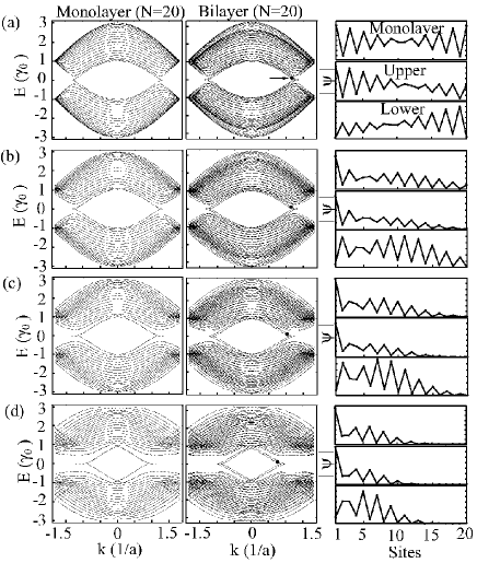
Figure 2: The energy band structures of zigzag monolayer (left panel) and bilayer (right panel) ribbons with $N=20$ for different magnetic flux through a hexagon (a) $\phi/\phi_{0}=0$, (b) $\phi/\phi_{0}=1/200$, (c) $\phi/\phi_{0}=1/100$ and (d) $\phi/\phi_{0}=1/50$. The corresponding wave functions at the energy represented by full circles are shown to the right (the top figure for each $\phi/\phi_{0}$ shows the wave function of the monolayer, while below, the wave functions of the upper and the lower layer are shown).

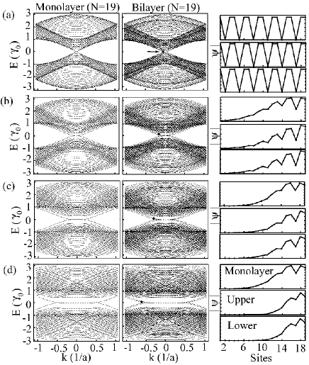
Figure 3: The energy band structures of metallic armchair monolayer (left panel) and bilayer (right panel) ribbons with $N=19$ for (a) $\phi/\phi_{0}=0$, (b) $\phi/\phi_{0}=1/200$, (c) $\phi/\phi_{0}=1/100$ and (d) $\phi/\phi_{0}=1/50$. The corresponding wave functions are shown to the right.

In Figs. 2 and 3 we present the energy band structures of respectively zigzag and armchair BGNs with $N=20,19$ and the corresponding wave functions for the values of magnetic flux $\phi/\phi_{0}=0,1/200,1/100,1/50$. Dispersion relations of the corresponding monolayer GNRs are plotted for comparison. As expected, the band structure of BGNs corresponds to two superimposed and somewhat deformed band structures of individual monolayer GNRs. To understand this character, we first assume that the two graphene layers of a bilayer system are decoupled. The system is therefore expected to behave as two isolated monolayer GNRs with all bands in the dispersion relation being doubly degenerate. By turning on the coupling between the two layers the degeneracy of the states is then lifted by the presence of the coupling, with the degree of splitting depending on the coupling strength. This is in a close analogy to a textbook example of a coupled quantum wells, where the splitting of the quantum well states depends on the strength of the barriers separating the wells. For the case of BGNs the coupling between layers is given by the hopping integrals $\gamma_{1}$ and $\gamma_{3}$ whose magnitudes ($\sim 0.3-0.4$ $eV$) determine the value of splitting of the corresponding monolayer bands.

The features of the band structure of BGNs at $B=0$ outlined above persist in the presence of a magnetic field. As $B$ increases to $\sim\phi/\phi_{0}=1/200$ the bands close to the Dirac points begin to flatten. This represents the onset of Landau level formation when the classical cyclotron radius $r_{c}$ for the low-velocity states (i.e. for those close to the Dirac points) becomes smaller than the ribbon width ( $r_{c}=\hbar k/eB=kl_{B}^{2},$ $l_{B}=\sqrt{\hbar/eB}$ (=1.3 nm at $\phi/\phi_{0}=1/200$) being the magnetic length). As the field is increased to $\phi/\phi_{0}=1/50$, the cyclotron motion dominates and the Landau levels become well developed.

It is interesting to note that similar to the case of monolayer GNRs, partly flat bands at $E=0$ exist in the band structures of the zigzag BNGs corresponding to the localized states on each edge, see Fig. 2. Compared to the monolayer cases, the number of edge states is doubled for each edge in bilayer ribbons. A detailed theoretical treatment of edge states in bilayer systems has been made recently Castro2008 .

Figures 2,3 also show some representative wave functions for different magnetic fields. As expected, the wave functions in the BGNs closely follow the corresponding wave functions of the monolayer GNRs. As the magnetic field increases, the wave functions are pushed towards the ribbon edges, signaling the formation of the familiar magnetic edge states which correspond to classical skipping orbits Ferry .

It should be noted that our nanoribbons are rather narrow and therefore the onset of the formation of the Landau levels (when the magnetic length $l_{D}$ becomes comparable to the ribbon’s width) can be reached only for an unrealistically high magnetic fields (for example, $\phi/\phi_{0}=1/50$ corresponds to $B=400$ T). In realistic experimental samples of submicron width, the formation of Landau levels scales down to much smaller magnetic fields. Due to computational limitations, however, it is rather impractical to consider wider ribbons and in the present study we therefore consider the same physics at higher fields.

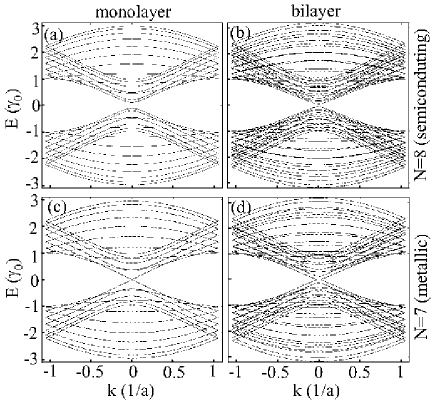
Figure 4: The energy bands of semiconducting and metallic armchair nanoribbons in $B=0$: (a) monolayer with $N=8$; (b) bilayer with $N=8$. In (c) and (d), the band structures of the monolayer and bilayer systems with $N=7$ are shown.

The electronic properties of armchair graphene nanoribbons depend sensitively on the ribbon width. The GNRs are metallic when $N-1$ is a multiple of $3$; otherwise, there is an energy gap between the conduction and valence band. Fig. 4(a-b) displays the band structures of the armchair BGN and GNR at $B=0$ with $N=8,7$. It is evident that both the monolayer and bilayer graphene ribbons with $N=8$ possess a bandgap around the zero-energy point. However, the energy gap of the BGN is narrower than that of the monolayer GNR even though they have the identical width. For the armchair BGN and GNR with $N=7$, the band structures show metallic characteristics as shown in Fig. 4(c) and (d). In contrast to the linear dispersion relation near the Dirac point in the monolayer GNR (Fig. 4(c)), the armchair BGN (Fig. 4(d)) shows a parabolic dispersion relation near the zero-energy point, which leads to new elementary excitations called massive Dirac fermions. These massive non-relativistic particles are chiral and can be described by an off-diagonal, Dirac-like Hamiltonian as the continuum limit of the tight-binding model Mccann2006 . This Hamiltonian of the bulk bilayer system gives rise to two parallel parabolic bands separated by an amount of $\sim\gamma_{1}$ close to the zero-energy point, which is consistent with our observations for nanoribbon structures.

III.2 Conductance quantization

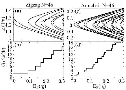
Figure 5: Upper panels: the energy spectra for the zigzag (a) and armchair (c) bilayer ribbons with $N=46$. (For the zigzag ribbon only the branches in the vicinity of one Dirac point are shown). Lower panels: The energy dependence of the zero-temperature conductance of the ideal zigzag (b) and armchair (d) ribbons associated with the energy spectra.

Now we are in the position to study the transport properties of BGNs. In clean ideal nanoribbons the conductance is determined by the number of propagating modes at the Fermi energy. Each spin-degenerate propagating mode contributes to the total conductance by the conductance unit $G_{0}=2e^{2}/h.$ Figure 5 shows the energy spectra for zigzag and armchair BGNs with $N=46$ and a corresponding conductance as a function of the Fermi energy at $B=0$. Note that analytical expressions for the conductance quantization in monolayer GNR were provided by Onipko Onipko who showed that the conductance of the monolayer GNRs is given by $G_{GNR}^{Z}=2(n+1/2)G_{0}$ for the zigzag ribbons and $G_{GNR}^{A}=nG_{0}$ for the armchair ribbons, where the integer number $n=0,1,2,\cdots$. Our calculations shows that the corresponding conductance of the zigzag and armchair bilayer ribbons is given respectively by $G_{BGN}^{Z}=2(n+1)G_{0}$ and $G_{BGN}^{A}=nG_{0}$, see Fig. 5. The minimum conductance of an ideal zigzag BGN is $2G_{0},$ whereas the minimum conductance of an ideal metallic armchair BGN is $G_{0}.$

Note that the conductance steps are not equidistant along the energy axis. For example, for the armchair BGN steps at $G_{0}$, $3G_{0}$, and $5G_{0}$ are more pronounced than those at $2G_{0}$, $4G_{0}$, and $6G_{0}$. The widths of conductance steps are determined by the energy scale between the successive modes in the energy spectrum, which in turn depends on the ribbon width and the energy interval. In wider armchair BGNs, some conductance quantization steps are poorly resolved or even unresolved which might lead to an apparent quantization in units of $2G_{0}$.

IV Effect of edge disorder on the conductance and localization length

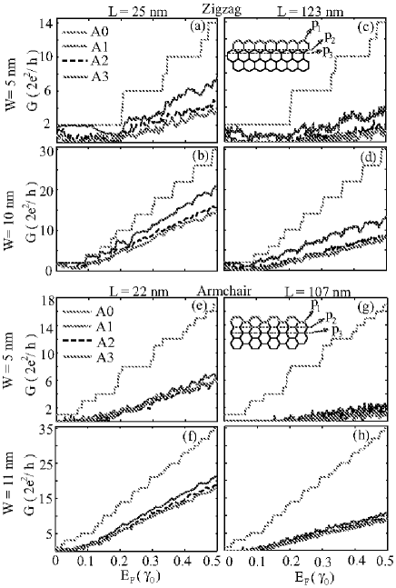
Figure 6: (Color online) The conductance as a function of the Fermi energy with varying edge disorder for different widths and lengths. Three typical disorder strengths are considered: $A0$: perfect edges; $A1$: $p_{1}=0.1$, $p_{2}=p_{3}=0$; $A2$: $p_{1}=0.3$, $p_{2}=0.2$ and $p_{3}=0.1$; $A3$: $p_{1}=0.5$, $p_{2}=0.4$ and $p_{3}=0.3$. The insets show the positions of the atoms for removing with the probabilities $p_{1},p_{2},$ and $p_{3}$. (a)-(d) the zigzag BGNs with widths $5$ nm-$10$ nm and length $25$ nm-$123$ nm. (e)-(h) the armchair BGNs with widths $5$ nm-$11$ nm and lengths $22$ nm-$107$ nm.

In this section we calculate the conductance of realistic BGNs with edge defects that are created by random removal of carbon atoms from the edges of the upper and lower layers. It was shown previously that the edge disorder strongly affects the conductance of monolayer GNRs.Chen2007 ; Han2007 ; Areshkin ; Louis ; Gunlycke ; Li ; Querlioz ; Avouris ; Evaldsson2008 ; Mucciolo ; Basu2008 ; Stampfer2009 . In particular, it has been demonstrated that even very modest edge disorder is sufficient to strongly suppress the conductance and to induce the conduction energy gap in the vicinity of the Dirac point and to lift any difference in the conductance between nanoribbons of different edge geometry (i.e. zigzag and armchair) Evaldsson2008 ; Mucciolo . This was related to the pronounced edge-disorder-induced Anderson-type localization which leads to a strongly enhanced density of states at the edges and to blocking of conductive paths through the ribbonsEvaldsson2008 . In the present study we use the model for the edge disorder applied previously to monolayer GNRs Evaldsson2008 and compare the effect of the edge disorder on the conductance and the localization length of monolayer GNRs and BGNs. We model the missing atoms by setting the corresponding hopping matrix elements to zero. The edge roughness is controlled by three probabilities $p_{1}$, $p_{2}$, $p_{3}$. $p_{1}$ is the probability of a missing atom in the outermost row; $p_{i}(i=2,3)$ is the conditional probability for a missing atom in the $i$-th row away from the edge if at least one adjacent atom in row $(i-1)$ is missing, see the illustration in the inset of Fig. 6. As graphene is known to have few bulk defects in general Schedin we do not consider bulk vacancies. We also disregard the effect of hydrogen capture by dangling bonds at the edge, since it has been shown to be of minor importance for ribbons wider than a few nanometers Son ; Barone .

Figure 6 shows the conductance of zigzag and armchair BGNs of different lengths and widths as a function of the Fermi energy for four edge disorder strengths. The conductance of the BGNs shows the same qualitative features as the conductance of the monolayer GNRs Evaldsson2008 . The main feature is that a relatively small edge disorder strongly suppresses the conductance and completely destroys the quantization steps for both zigzag and armchair BGNs. As a result, no difference in the conductance is expected for realistic zigzag and armchair BGNs. Armchair BGNs show a well-pronounced transport gap in the vicinity of the charge neutrality point. As in the case of monolayer ribbons, the zigzag BGNs are more robust to this disorder-induced suppression of the conductance. This behavior has been related to the presence of the edge states in the zigzag nanoribbon close to the Dirac point Areshkin .

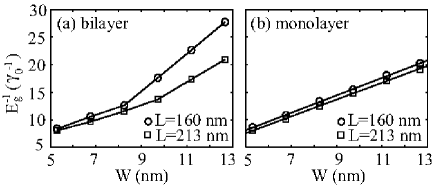
Figure 7: The inverse of the energy gap versus ribbon width for (a) armchair BGNs and (b) armchair monolayer GNRs. The energy gap $E_{g}$ is defined as the interval where $G\lesssim 10^{-3}\times 2e^{2}/h$.

Recent experiments and calculations have shown that the transport gap in monolayer GNRs is approximately proportional to the inverse of the ribbon width $W$ Han2007 ; Louis ; Querlioz ; Evaldsson2008 ; Mucciolo . In Fig. 7 we plot the inverse of the transport gap, $E_{g}^{-1},$ for the armchair BGNs and monolayer GNRs as a function of the ribbon width $W$. While for the monolayer ribbons $E_{g}^{GNR}\sim 1/W$, the corresponding transport gap $E_{g}^{BGN}$ for the bilayer ribbons shows a more rapid decrease as $W$ increases. This indicates that edge-disorder induced localization of the states is less pronounced in BGNs in comparison to GNRs. In order to elucidate this point further, we have performed a comparative study of the localization length $\xi$ as a function of the Fermi energy $E_{F}$in both systems, choosing nanoribbons of width $W=11\,\mathrm{nm}$, corresponding to $46$ atomic sites in $y$-direction. The vacancy probabilities have been set to $p_{1}=0.5$, $p_{2}=0.4$ and $p_{3}=0.3$, respectively. The nanoribbons are thus identical to that one of Fig. 6 (h), configuration $A3$. $\xi(E_{F})$ is determined by calculating the conductance $G$ as a function of the nanoribbon length $L$ for an ensemble of 5000 disorder configurations for each length. As the energy increases, the system is expected to undergo a transition from the strongly localized regime where the conductance decays exponentially as $L$ increases, to the Ohmic regime where $G\propto 1/L$. The conductance is expected to obey the scaling law

$$\ln(1+1/g)=L/\xi,$$ (4)

with the dimensionless conductance $g=G/(e^{2}/\pi\hbar)$ Anderson1980 . We find that for all energies, the simulated conductances can be fitted with high accuracy by Eq. (4), as exemplified in the inset of Fig. 8(c), with $\xi$ being the fit parameter. Fig. 8 (c) shows the localization length determined that way as a function of the Fermi energy for both monolayer and bilayer ribbons. Two regimes can be identified, depending on whether the Fermi energy $E_{F}$ is inside or outside the transport gap. For energies inside the transport gap, $|E_{F}|\lesssim E_{g},$ (with $E_{g}\approx 0.06\gamma_{0}$ for the particular system under study), $\xi$ is essentially independent of $E_{F}$ and comparable to $W$. In this interval, $\xi$ in the BGN is roughly a factor of $2$ larger than in the GNR. As $E_{F}$ increases above the transport gap, $\xi$ increases rapidly, while the difference in $\xi$ for the mono-and the bilayer system fluctuates around zero. We emphasize that these fluctuations are well above the noise level, due to the large ensemble used.

This behavior can be interpreted qualitatively as follows. Inside the transport gap, $|E_{F}|\lesssim E_{g}$, large disorder-induced potential barriers are present in each layer which hamper the electron transfer along the wire. If an electron encounters such a barrier in one layer, it can bypass it by hopping to the second layer. Because such a bypassing is apparently not possible in a system with a single layer the electrons are less localized in the BGNs.

Outside the transport gap, $|E_{F}|\gtrsim E_{g}$, conducting channels open up in both layers and therefore the interlayer transfer becomes less likely compared to the intralayer transfers. Because of this, electronic transport in each layer is much less affected by the presence of the neighboring level which results in similar localization lengths for the monolayer and the bilayer nanoribbons. The differences in $\xi$ for the mono- and the bilayer system mentioned above can be traced to the features in the dispersion relations corresponding to the opening of new propagating channels. A correlation between the dispersion relation and the behavior of $\xi(E)$ is clearly seen in Fig. 8. For example, the strong increase of $\xi$ between $0.06\gamma_{0}<E<0.1\gamma_{0}$ of the monolayer is related to the occupation of the second mode. As the energy (and therefore a number of modes) increases, the difference of $\xi(E)$ between mono- and bilayer nanoribbons diminishes.

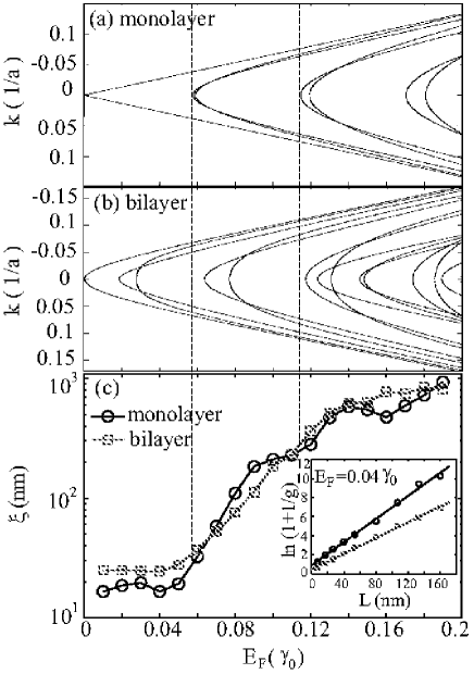
Figure 8: Bottom: The localization length $\xi$ as a function of the Fermi energy for a ribbon of the width $W=11$ nm. Inset: length dependence of $\ln(1+1/g)$. Top: The monolayer and bilayer dispersion relations for the corresponding nanoribbons with perfect edges.

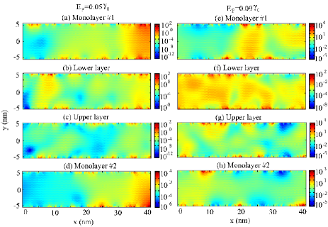
Figure 9: (Color online) The local density of states in representative parts of the edge disorder regions. (a) and (d) are the LDOS of two independent monolayer at $E_{F}=0.05\gamma_{0}$ (i.e. inside the transport energy gap) and evolve into (b) and (c), respectively, when the interlayer interaction is turned on. (e) and (h) are the LDOS of two independent monolayer at $E_{F}=0.09\gamma_{0}$ (i.e. outside the energy gap) and evolve into (f) and (g), respectively, when the interlayer interaction is turned on.

An inspection of a typical local density of states (LDOS) pattern of a representative member of the nanoribbon ensemble substantiates this interpretation of the properties of $\xi(E)$, see Fig. 9. We first generate two monolayer GNRs with the same concentration but different configurations of edge disorder, and then couple them to form the lower and the upper layers of a bilayer BGN. We then separately calculate the LDOS for these three structures (i.e. for two different monolayer GNRs and one BGR). The pronounced enhancement of the LDOS at the edges (note the logarithmic scale) and the substantial fluctuations at larger scales indicate Anderson localization as discussed in detail elsewhere Evaldsson2008 .

Figures 9 (a)-(d) show the LDOS plots for $E_{F}$ lying inside the energy gap. A comparison of the LDOS pattern shows an anticorrelation between the lower and upper layers of the BGN (i.e. the enhanced LDOS in one layer is accompanied by the suppressed LDOS in the second layer). At the same time, there is not much correlation between LDOS patterns of the BGN and the corresponding LDOSs of the monolayer GNRs. This is consistent with the interpretation presented above where the interlayer transfer is dominant such that the electrons encountering a potential barrier (which reduces the LDOS) in one layer, jump to the second layer and enhance the LDOS of the neighboring sites therein.

The LDOS patterns for a representative value of $E_{F}$ above the transport gap demonstrate that the intralayer transfer is dominant in this regime. Indeed, in this case a correlation can be seen between the LDOS patterns of the BGN and the corresponding LDOSs of the monolayer GNRs which signifies the presence of the open propagating channels in each layer. Note that there is also a certain correlation even between two layers in the BGN. For example, the lower layer of the BGN (Fig. 9(f)) shows some additional LDOS maxima which are not present in its constitutive monolayer $\#1$ (see Fig. 9(e)) but correlate to the LDOS maxima in the second layer of the BGN (Fig. 9 (g)). This correlation between layers indicates that due to the coupling between the layers the defects in the upper layer simply generate additional defects of comparable strength in the lower layer and vice versa.

Finally we note that no attempts were made to quantify the correlations in the LDOS patterns. We rather restricted ourselves to a visual inspection which explain qualitatively the behavior of $\xi(E_{F})$.

V Summary and conclusions

We have studied the electronic structures and transport properties of Bernal-type graphene bilayer nanoribbons using the recursive Green’s function technique. The band structures of the zigzag and armchair BGNs with uniform perpendicular magnetic fields have been computed for the entire energy regime of the $\pi$-bands. The calculated band structure corresponds to two superimposed and somewhat deformed band structures of individual monolayer GNRs. The splitting between the corresponding monolayer bands is of the order of $\sim 0.3-0.4$ eV and is determined by the interlayer hopping integrals $\gamma_{1}$ and $\gamma_{3}$ providing coupling between the layers. The conductance of the clean (disorder-free) zigzag system is quantized as $2(n+1)G_{0}$, whereas the clean armchair system is quantized as $nG_{0}$ with $G_{0}=2e^{2}/h$ being the conductance unit and $n$ an integer number. Furthermore, the effect of edge disorder, which is highly relevant in realistic samples, has been investigated. As in the case of monolayer ribbons, a relatively small edge disorder strongly suppress the conductance of the BGN, introduces the transport energy gap in the vicinity of the charge neutrality point and completely destroys the quantization steps for both zigzag and armchair BGNs. We calculate the localization length as a function of the Fermi energy $E_{F}$ and identify two distinct regimes depending on whether $E_{F}$ is inside or outside the transport gap. The localization length inside the transport gap is larger in BGNs than in GNRs with identical edge roughness. This difference, however, disappears at energies above the transport gap.

Appendix A Hamiltonian and coupling matrices

In this appendix we provide explicit forms of the hamiltonians for the ${i}$-th slices $h_{i}$ and coupling matrices $U$. $V_{i}^{\prime}$ denotes the potential on the site $i$ in the upper layer and $V_{i}$ the potential on $i$-th site in the lower layer. The diagonal blocks of the matrices correspond to the Hamiltonians of layers, and off-diagonal blocks give the interlayer interactions.

A.1 Zigzag edge

$$h_{1}=\left(\begin{array}[]{ccccc|ccccc}V_{1}^{\prime}&\gamma_{0}&0&0&\cdots&\gamma_{1}&0&0&0&\cdots\\ \gamma_{0}&V_{2}^{\prime}&0&0&&0&\gamma_{3}&0&0&\\ 0&0&V_{3}^{\prime}&\gamma_{0}&&0&0&\gamma_{1}&0&\\ 0&0&\gamma_{0}&V_{4}^{\prime}&&0&0&0&\gamma_{3}&\\ \vdots&&&&\ddots&\vdots&&&&\ddots\\ \hline\cr\gamma_{1}&0&0&0&\cdots&V_{1}&0&0&0&\cdots\\ 0&\gamma_{3}&0&0&&0&V_{2}&\gamma_{0}&0&\\ 0&0&\gamma_{1}&0&&0&\gamma_{0}&V_{3}&0&\\ 0&0&0&\gamma_{3}&&0&0&0&V_{4}&\\ \vdots&&&&\ddots&\vdots&&&&\ddots\\ &&&&&&&&&\end{array}\right)$$ (5)

$$h_{2}=\left(\begin{array}[]{ccccc|ccccc}V_{1}^{\prime}&0&0&0&\cdots&\gamma_{3}&0&0&0&\cdots\\ 0&V_{2}^{\prime}&\gamma_{0}&0&&0&\gamma_{1}&0&0&\\ 0&\gamma_{0}&V_{3}^{\prime}&0&&0&0&\gamma_{3}&0&\\ 0&0&0&V_{4}^{\prime}&&0&0&0&\gamma_{1}&\\ \vdots&&&&\ddots&\vdots&&&&\ddots\\ \hline\cr\gamma_{3}&0&0&0&\cdots&V_{1}&\gamma_{0}&0&0&\cdots\\ 0&\gamma_{1}&0&0&&\gamma_{0}&V_{2}&0&0&\\ 0&0&\gamma_{3}&0&&0&0&V_{3}&\gamma_{0}&\\ 0&0&0&\gamma_{1}&&0&0&\gamma_{0}&V_{4}&\\ \vdots&&&&\ddots&\vdots&&&&\ddots\\ &&&&&&&&&\end{array}\right)$$ (6)

$$U^{12}=(U^{21})^{+}=\left(\begin{array}[]{ccccc|ccccc}\gamma_{0}&0&0&0&\cdots&0&0&0&0&\cdots\\ 0&\gamma_{0}&0&0&&\gamma_{3}&0&0&0&\\ 0&0&\gamma_{0}&0&&0&0&0&0&\\ 0&0&0&\gamma_{0}&&0&0&\gamma_{3}&0&\\ \vdots&&&&\ddots&&&&&\ddots\\ \hline\cr 0&0&0&0&\cdots&\gamma_{0}&0&0&0&\cdots\\ 0&0&\gamma_{3}&0&&0&\gamma_{0}&0&0&\\ 0&0&0&0&&0&0&\gamma_{0}&0&\\ 0&0&0&0&&0&0&0&\gamma_{0}&\\ \vdots&&&&\ddots&\vdots&&&&\ddots\\ &&&&&&&&&\end{array}\right)$$ (7)

A.2 Armchair edge

$$h_{1\sim 4}=\left(\begin{array}[]{ccccc|ccccc}V_{1}^{\prime}&0&0&0&\cdots&&&&&\\ 0&V_{2}^{\prime}&0&0&&&&&&\\ 0&0&V_{3}^{\prime}&0&&&&0&&\\ 0&0&0&V_{4}^{\prime}&&&&&&\\ \vdots&&&&\ddots&&&&&\\ \hline\cr&&&&&V_{1}&0&0&0&\cdots\\ &&&&&0&V_{2}&0&0&\\ &&0&&&0&0&V_{3}&0&\\ &&&&&0&0&0&V_{4}&\\ &&&&&\vdots&&&&\ddots\\ &&&&&&&&&\end{array}\right)$$ (8)

$$U^{01}=(U^{10})^{+}=\left(\begin{array}[]{ccccc|ccccc}\gamma_{0}&0&0&0&\cdots&&&&&\\ 0&\gamma_{0}&0&0&&&&&&\\ 0&0&\gamma_{0}&0&&&&0&&\\ 0&0&0&\gamma_{0}&&&&&&\\ \vdots&&&&\ddots&&&&&\\ \hline\cr\gamma_{3}&0&0&0&\cdots&\gamma_{0}&0&0&0&\cdots\\ \gamma_{3}&\gamma_{3}&0&0&&0&\gamma_{0}&0&0&\\ 0&\gamma_{3}&\gamma_{3}&0&&0&0&\gamma_{0}&0&\\ 0&0&\gamma_{3}&\gamma_{3}&&0&0&0&\gamma_{0}&\\ \vdots&&&&\ddots&\vdots&&&&\ddots\\ &&&&&&&&&\end{array}\right)$$ (9)

$$U^{12}=(U^{21})^{+}=\left(\begin{array}[]{ccccc|ccccc}\gamma_{0}&\gamma_{0}&0&0&\cdots&\gamma_{3}&0&0&0&\cdots\\ 0&\gamma_{0}&\gamma_{0}&0&&0&\gamma_{3}&0&0&\\ 0&0&\gamma_{0}&\gamma_{0}&&0&0&\gamma_{3}&0&\\ 0&0&0&\gamma_{0}&&0&0&0&\gamma_{3}&\\ \vdots&&&&\ddots&\vdots&&&&\ddots\\ \hline\cr\gamma_{1}&0&0&0&\cdots&\gamma_{0}&0&0&0&\cdots\\ 0&\gamma_{1}&0&0&&\gamma_{0}&\gamma_{0}&0&0&\\ 0&0&\gamma_{1}&0&&0&\gamma_{0}&\gamma_{0}&0&\\ 0&0&0&\gamma_{1}&&0&0&\gamma_{0}&\gamma_{0}&\\ \vdots&&&&\ddots&\vdots&&&&\ddots\\ &&&&&&&&&\end{array}\right)$$ (10)

$$U^{23}=(U^{32})^{+}=\left(\begin{array}[]{ccccc|ccccc}\gamma_{0}&0&0&0&\cdots&&&&&\\ 0&\gamma_{0}&0&0&&&&&&\\ 0&0&\gamma_{0}&0&&&&0&&\\ 0&0&0&\gamma_{0}&&&&&&\\ \vdots&&&&\ddots&&&&&\\ \hline\cr\gamma_{3}&\gamma_{3}&0&0&\cdots&\gamma_{0}&0&0&0&\cdots\\ 0&\gamma_{3}&\gamma_{3}&0&&0&\gamma_{0}&0&0&\\ 0&0&\gamma_{3}&\gamma_{3}&&0&0&\gamma_{0}&0&\\ 0&0&0&\gamma_{3}&&0&0&0&\gamma_{0}&\\ \vdots&&&&\ddots&\vdots&&&&\ddots\\ &&&&&&&&&\end{array}\right)$$ (11)

$$U^{34}=(U^{43})^{+}=\left(\begin{array}[]{ccccc|ccccc}\gamma_{0}&0&0&0&\cdots&\gamma_{3}&0&0&0&\cdots\\ \gamma_{0}&\gamma_{0}&0&0&&0&\gamma_{3}&0&0&\\ 0&\gamma_{0}&\gamma_{0}&0&&0&0&\gamma_{3}&0&\\ 0&0&\gamma_{0}&\gamma_{0}&&0&0&0&\gamma_{3}&\\ \vdots&&&&\ddots&\vdots&&&&\ddots\\ \hline\cr\gamma_{1}&0&0&0&\cdots&\gamma_{0}&\gamma_{0}&0&0&\cdots\\ 0&\gamma_{1}&0&0&&0&\gamma_{0}&\gamma_{0}&0&\\ 0&0&\gamma_{1}&0&&0&0&\gamma_{0}&\gamma_{0}&\\ 0&0&0&\gamma_{1}&&0&0&0&\gamma_{0}&\\ \vdots&&&&\ddots&\vdots&&&&\ddots\\ &&&&&&&&&\end{array}\right)$$ (12)

Appendix B Formalism

In this Appendix we provide main formulas used for calculation of the dispersion relations, Bloch states and their velocities and the transmission and reflection amplitudes for the scattering problem for bilayer graphene ribbons. All these formulas represent a straighforward generalization of the corresponding formular derived in Ref. [Xu2008, ] for monolayer ribbons.

The band structure is computed by solving a eigenvalue of the form

$$T_{1}^{-1}T_{2}\left(\begin{array}[]{c}\psi_{1}\\ \psi_{0}\end{array}\right)=e^{ikM}\left(\begin{array}[]{c}\psi_{1}\\ \psi_{0}\end{array}\right)$$ (13)

with $M$ being the periodicity ($M=2$ and $4$ for the zigzag and armchair BGRs respectively),

$$T_{1}=\begin{pmatrix}-G_{\mathrm{cell}}^{1,M}U^{M,M+1}&\;0\\ -G_{\mathrm{cell}}^{M,M}U^{M,M+1}&\;I\end{pmatrix},\;T_{2}=\begin{pmatrix}-I&\;G_{\mathrm{cell}}^{1,1}U^{1,0}\\ 0&\;G_{\mathrm{cell}}^{M,1}U^{1,0}\end{pmatrix}$$

$I$ being the unitary matrix.

This eigenvalue problem Eq. (13) gives the eigenfunctions $\psi^{\alpha}$, $1\leq\alpha\leq 2N$ and the set of Bloch eigenvectors $\left\{k_{\alpha}\right\}$ which includes both propagating and evanescent states. The latter can be easily identified by a non-zero imaginary part. In order to separate right- and left-propagating states, $k_{\alpha}^{+}$ and $k_{a}^{-},$ we compute the group velocities of the Bloch states $v_{\alpha}=\frac{\partial E}{\partial k_{\alpha}}$, whose signs determine the direction of propagation (‘+’ stands for the right-propagating and ‘-’ for the left propagating states).

Starting from the Schrödinger equation and using a definition of the group velocity, we obtain the group velocity for graphene nanoribbons

$$v=\frac{1}{M}\sum_{i=1}^{M}\frac{\partial}{\partial k}\left[\frac{\langle\psi_{i}|H|\psi\rangle}{|\varphi_{i}|^{2}}\right]$$ (14)

where the summation is performed over all slices of the unit cell, and

$$\varphi_{i}=(\varphi_{i,1};...;\varphi_{i,2N})^{T}$$ (15)

is a vector composed of the matrix elements $\varphi_{i,j}=$ $\langle 0a_{i,j}|\varphi\rangle$ (Note that vectors $\varphi_{i}$ can be obtained from $\psi_{i}$ via the relation $\psi_{i}=e^{iki}\varphi_{i}$).

To account for the effects of the leads, one needs to calculate the surface Green’s function. The latter equations can be used for determination of $\Gamma_{r}$,

$$\Gamma_{r}U^{1,0}=\Psi_{1}\Psi_{0}^{-1},$$ (16)

where $\Psi_{1}$ and $\Psi_{0}$ are the square matrixes composed of the matrix-columns $\psi_{1}^{\alpha}$ and $\psi_{0}^{\alpha},$ ($1\leq\alpha\leq 2N),$ Eq. (13), i.e. $\Psi_{1}=(\psi_{1}^{1},...,\psi_{1}^{2N});$ $\Psi_{0}=(\psi_{0}^{1},...,\psi_{0}^{2N}).$ The expression for the left surface Greens function $\Gamma_{l}$ (i.e. the surface function of the semiinfinite ribbon open to the right) is derived in a similar fashion,

$$\Gamma_{l}U^{M,M+1}=\Psi_{M}\Psi_{M+1}^{-1},$$ (17)

where the matrixes $\Psi_{M}$ and $\Psi_{M+1}$ are defined in a similar way as $\Psi_{1}$ and $\Psi_{0}$ above.

The transmission and reflection amplitudes is calculated using the expressions:

$$\Phi_{1}T=-G^{L,0}(U^{0,1}\Psi_{1}-\Gamma_{l}^{-1}\Phi_{0}).\\$$ (18)

$$\Phi_{0}R=-G^{0,0}(U^{0,1}\Psi_{1}-\Gamma_{l}^{-1}\Phi_{0})-\Phi_{0}.$$ (19)

The matrices $T$ and $R$ with the dimension 2$N\times N_{\mathrm{prop}}$ are composed of the transmission and reflection amplitudes $t_{\beta\alpha}$ and $r_{\beta\alpha}$, (with $N_{\mathrm{prop}}$ being the number of propagating modes in the leads). The Green’s functions $G^{M+1,0}$ and $G^{0,0}$ are obtained from the standard recursive technique based on the Dyson’s equation Ferry . The transmission and reflection are related to their amplitudes by $(T)_{\beta\alpha}=v_{\beta}^{+}/v_{\alpha}^{+}|t_{\beta\alpha}|^{2}$ and $(R)_{\beta\alpha}=v_{\beta}^{-}/v_{\alpha}^{+}|r_{\beta\alpha}|^{2}$.

References

- (1) K.S. Novoselov, A. K. Geim, S. V. Morozov, D. Jiang, Y. Zhang, S. V. Dubonos, I. V. Grigorieva, A. A. Firsov, Science 306, 666 (2004).
- (2) M. I. Katsnelson, K. S. Novoselov and A. K. Geim, Nature Physics, 2, 620 (2006).
- (3) For a review, see A. H. Castro Neto, F. Guinea, N. M. R. Peres, K. S. Novoselov, and A. K. Geim, Rev. Mod. Phys. 81, 109 (2009).
- (4) Katsunori Wakabayashi, Mitsutaka Fujita, Hiroshi Ajiki, Manfred Sigrist, Phys. Rev. B 59, 8271 (1999).
- (5) L. Brey and H. A. Fertig, Phys. Rev. B 73, 235411 (2006).
- (6) F. Muñoz-Rojas, D. Jacob, J. Fernández-Rossier, and J. J. Palacios, Phys. Rev. B 74, 195417 (2006).
- (7) C. H. Lewenkopf, E. R. Mucciolo, A. H. Castro Neto, Phys. Rev. B 77, 081410(R) (2008).
- (8) Z. Chen, Y.-M. Lin, M. J. Rooks and P. Avouris, Physica E 40, 228 (2007).
- (9) M. Y. Han, B. Ozyilmaz, Y. Zhang, and P. Kim, Phys. Rev. Lett. 98, 206805 (2007).
- (10) Xinran Wang, Yijian Ouyang, Xiaolin Li, Hailiang Wang, Jing Guo, and Hongjie Dai, Phys. Rev. Lett. 100, 206803 (2008).
- (11) A. De Martino, L. Dell’Anna, and R. Egger, Phys. Rev. Lett. 98, 066802 (2007).
- (12) Hengyi Xu, T. Heinzel, M. Evaldsson, and I.V. Zozoulenko, Phys. Rev. B 77, 245401 (2008).
- (13) M. Ramezani Masir, P. Vasilopoulos, A. Matulis, and F. M. Peeters, Phys. Rev. B 77, 235443 (2008).
- (14) R. N. Costa Filho, G. A. Farias, and F. M. Peeters, Phys. Rev. B 76, 193409 (2007), and references therein.
- (15) M. Evaldsson, I. V. Zozoulenko, Hengyi Xu, and T. Heinzel, Phys. Rev. B 78, 161407(R) (2008).
- (16) Yuanbo Zhang, Yan-Wen Tan, Horst L. Stormer, and Philip Kim, Nature (London) 438, 201 (2005).
- (17) K. S. Novoselov, A. K. Geim, S. V. Morozov, D. Jiang, M. I. Katsnelson, I. V. Grigorieva, S. V. Dubonos, and A. A. Firsov, Nature (London) 438, 197 (2005).
- (18) V. P. Gusynin and S. G. Sharapov, Phys. Rev. Lett. 95, 146801 (2005).
- (19) N. M. R. Peres, F. Guinea, and A. H. Castro Neto, Phys. Rev. B 73, 125411 (2006).
- (20) Edward McCann, Phys. Rev. B 74, 161403(R) (2006).
- (21) K. Kechedzhi, V. I. Fal’ko, E. McCann, and B.L. Altshuler, Phys. Rev. Lett. 98, 176806 (2007).
- (22) I. Snymann and C. W. J. Beenakker, Phys. Rev. B 75, 045322 (2007).
- (23) D. S. L. Abergel and Vladimir I. Fal’ko, Phys. Rev. B 75, 155430 (2007).
- (24) Y. H. Lai, J. H. Ho, C. P. Chang, and M. F. Lin, Phys. Rev. B 77, 085426 (2008).
- (25) E. V. Castro, N. M. R. Peres, J. M. B. Lopes dos Santos, A. H. Castro Neto, and F. Guinea, Phys. Rev. Lett. 100, 026802 (2008).
- (26) R. V. Gorbachev, F. V. Tikhonenko, A. S. Mayorov, D. W. Horsell, and A. K. Savchenko, Phys. Rev. Lett. 98, 176805 (2007).
- (27) J. Nilsson, A.H. Castro Neto, F. Guinea, and N.M.R. Peres, Phys. Rev. B 78, 045405 (2008).
- (28) M. I. Katsnelson, Eur. Phys. J. B 52, 151 (2006).
- (29) J. Cserti, Phys. Rev. B 75, 033405 (2007).
- (30) J. B. Oostinga, H. B. Heersche, X. Liu, A. F. Morpurgo, and L. M. K. Vandersypen, Nat. Mat, 7, 151 (2007).
- (31) E. V. Castro, K. S. Novoselov, S. V. Morozov, N. M. R. Peres, J. M. B. Lopes dos Santos, J. Nilsson, F. Guinea, A. K. Geim, and A. H. Castro Neto, Phys. Rev. Lett. 99, 216802 (2007).
- (32) E. McCann, Phys. Rev. B 74, 161403(R) (2006).
- (33) E. V. Castro, N. M. R. Peres, T. Stauber, and N. A. P. Silva, Phys. Rev. Lett. 100, 186803 (2008).
- (34) V. I. Fal’ko, Phi. Trans. R. Soc. A 366, 205 (2008).
- (35) J. Nilsson and A.H. Castro Neto, Phys. Rev. Lett. 98, 126801 (2007).
- (36) J. Nilsson, A.H. Castro Neto, F. Guinea, and N.M.R. Peres, Phys. Rev. Lett. 97, 266801 (2006).
- (37) J. Nilsson, A. H. Castro Neto, F. Guinea, and N. M. R. Peres, Phys. Rev. B 76, 165416 (2007).
- (38) J. Fernandez-Rossier, J. J. Palacios, and L. Brey, Phys. Rev. B 75, 205441 (2007).
- (39) P. G. Silvestrov and K. B. Efetov, Phys. Rev. B 77, 155436 (2008).
- (40) D. A. Areshkin, D. Gunlycke, and C. T. White, Nano. Lett. 7, 204 (2007).
- (41) E. Louis, J. A. Vergés, F. Guinea, and G. Chiappe, Phys. Rev. B 75, 085440 (2007).
- (42) D. Gunlycke, D. A. Areshkin, and C. T. White, Appl. Phys. Lett. 90, 142104 (2007).
- (43) T. C. Li and S.-P. Lu, Phys. Rev. B 77, 085408 (2008).
- (44) D. Querlioz, Y. Apertet, A. Valentin, K. Huet, A. Bournel, S. Galdin-Retailleau, and P. Dollfus, Appl. Phys. Lett. 92, 042108 (2008).
- (45) Yu-Ming Lin, Vasili Perebeinos, Zhihong Chen, and Phaedon Avouris, Phys. Rev. B 78, 161409(R) (2008).
- (46) E. R. Mucciolo, A. H. Castro Neto, and C. H. Lewenkopf, Phys. Rev. B 79, 075407 (2009).
- (47) D. Basu, M. J. Gilbert, L. F. Register, and S. K. Banerjee, A. H. MacDonald, Appl. Phys. Lett. 92, 042114 (2008).
- (48) C. Stampfer, J. Güttinger, S. Hellmüller, F. Molitor, K. Ensslin, and T. Ihn, Phys. Rev. Lett. 102, 056403 (2009).
- (49) D. K. Ferry and S. M. Goodnick, Transport in Nanostructures, (Cambridge University Press, Cambridge, 1997);
- (50) A. I. Rahachou and I. V. Zozoulenko, Phys. Rev. B 72, 155117 (2005).
- (51) A. Onipko, Phys. Rev. B 78, 245412 (2008).
- (52) F. Schedin, A. K. Geim, S. V. Morozov, E. W. Hill, P. Blake, M. I. Katsnelson, and K. S. Novoselov, Nature Mater. 6, 652 (2007).
- (53) Y.-W. Son, M. L. Cohen, and S. G. Louie, Phys. Rev. Lett. 97, 216803 (2006).
- (54) V. Barone, O. Hod, and G. E. Scuseria, Nano Lett. 6, 2748 (2006).
- (55) P. W. Anderson, D. J. Thouless, E. Abrahams, D. S. Fisher, Phys. Rev. B 22, 3519 (1980); P. A. Lee, T. V. Ramakrishnan, Rev. Mod. Phys. 57, 287 (1985).