Local Risk Decomposition for High-frequency Trading Systems

Abstract

In the present work we address the problem of evaluating the historical performance of a trading strategy or a certain portfolio of assets. Common indicators such as the Sharpe ratio and the risk adjusted return have significant drawbacks. In particular, they are global indices, that is they do not preserve any local information about the performance dynamics either in time or for a particular investment horizon. This information could be fundamental for practitioners as the past performance can be affected by the non-stationarity of financial market. In order to highlight this feature, we introduce the local risk decomposition (LRD) formalism, where dynamical information about a strategy’s performance is retained. This framework, motivated by the multi-scaling techniques used in complex system theory, is particularly suitable for high-frequency trading systems and can be applied into problems of strategy optimization.

1 Introduction

Measuring the past performance of a trading system or a portfolio of assets is one of the most important issues for financial practitioners and portfolio managers. Evaluating performances heavily depends on estimating “risk”. In the past different measures has been proposed but there is no general agreement about which one is the most robust estimator for the “quality” of a trading strategy (Dacorogna01, ).

In this paper, we contribute to the risk-adjusted performance measurement subject by introducing a two dimensional decomposition of the profit and loss series, PandL, of a trading strategy. Based on this decomposition we can define a set of local performance indicators, where “local” refers to both time and investment horizon. Global indicators are then obtained via the convolution of the decomposed signal with user-specified kernels. The choice of the kernels, as well as their parameters, can highlight specific features of the trading dynamics.

The relevance of this multi-scale framework, originally developed in physics for the study of complex system (Bouchaud99, ; Sornette04, ; Voit05, ), in the contest of risk-adjusted measures is justified by the possible non-stationarity of the trading performances. In fact, it is a well known fact that some strategies work well just under some specific market condition or for a limited period of time when the related arbitrage inefficiency has not extensively exploited yet.

The issue of stability in performance metrics when facing non-stationary returns has been also addressed in econometric literature, with particular emphasis on the Sharpe ratio (Sharpe94, ), where different nonparametric methods have been proposed in order to give more “stable” estimates, see (Dowd00, ; Mukherjee04, ; Woehrmann05, ; Ledoit08, ) for example. Our approach differs from the formers in many respects. Firstly, we do not introduce a new specific risk-adjusted measure but rather a framework where to apply the already existing ones. Secondly, the risk associated with a strategy is not only considered as time dependent but also as “scale” dependent. Lastly, the fluctuations related to the risk performance are estimated around local trends in order to remove any possible bias due to some particular market condition during the period under consideration.

The paper is structured as following: in the next section we briefly introduce some standard indicators and point out their drawbacks. In Sec. 3 we introduce our local risk decomposition, LRD, while in Sec. 4 we apply the method to the performance of different trading systems and we highlight the advantages of using the LRD method if compared to standard indicators. Discussions and conclusions are left for the last section.

2 Risk performance measures

The performance of a trading strategy are characterized by two key quantities: the cumulative return over time, represented by the PandL time series, and the risk incurred in using it. While it is intuitive to associate profitability with the goodness of a trading strategy, high profits can be due to lucky trades or temporary favorable market conditions. This is the reason why investors tend to monitor the performance of their trading systems in time in order to recognize a possible deterioration in their strategy. The risk-adjusted performance measures proposed in literature, see for example Dacorogna01 , attempt to assert the quality of a trading system by assuming that an investor will make his/her decision based not only on the past returns but also on their fluctuations. Clearly the “amplitude” of fluctuations that a trader can tolerate depends on his/her personal appetite for risk and is thus subjective. However, investors tend to be risk adverse and, in practice, a trading strategy in order to be “acceptable” will have to display not only a good annualized profit but also a smooth cumulative return or PandL. In other words, the risk related to the fluctuation around the average return has to be small.

One of the most popular risk performance measures used in finance is the Sharpe ratio (Sharpe94, ), defined as

$$S=A\frac{\langle r\rangle}{\sigma_{r}},$$ (1)

where $\langle r\rangle$ is the average return and $\sigma_{r}$ is its standard deviation. The annualization factor, $A$, is $\sqrt{252}$ for daily returns or $\sqrt{12}$ for monthly. The Sharpe ratio, despite being widely used, has two notable drawbacks (Dacorogna01, ) among which

1. It is numerically unstable for small values of $\sigma_{r}$,

2. It does not reveal any information about the dynamics of the returns.

The last point is of central interest in the present work. In fact, since the high-frequency dynamics of the stock market is not stationary in time (Bartolozzi06, ; Bartolozzi07, ; Bartolozzi07b, ), the performance of trading systems can be subjected to similar trends.

Another widely used performance measure is the risk adjusted return, defined as

$$R_{\beta}=\langle r\rangle-\beta\,\sigma_{r}.$$ (2)

This indicator, derived from utility theory (Dacorogna01, ; Bailey05, ), is not affected by numerical singularities. However, it depends on the subjective risk strength factor, $\beta$. Furthermore, along with the Sharpe ratio, it does not reveal any information about the evolution of the PandL.

In the next section we introduce a multi-scale framework for estimating a risk-adjusted performance measure based on recent work in complex system theory (Sornette04, ). This framework, while employing elementary block measures similar to Eqs. (1) and (2), also retains time and horizon information which can be fundamental in a strategy selection problem.

3 The Local Risk Decomposition

In order to tackle the problem of non-stationarity of the performance of market strategies, we introduce the Local Risk Decomposition (LRD). The underlying idea of this method is to extrapolate a risk measure based on the local fluctuations of the PandL, both in time and scale (or investment horizon). This concept is similar to the detrended fluctuation analysis, recently proposed to extract correlations from non-stationary time series in the context of DNA nucleotides sequences (Peng93, ), and successively applied in finance by several authors (Cizeau97, ; Liu97, ; Vandewalle97, ; Liu99, ; Janosi99, ; Gopikrishnan00, ; Gopikrishnan01, ; Muniandy01, ; Matia02, ; Costa03, ; Grech04, ; Ivanov04, ; Eisler06, ; Bartolozzi07, ).

The LRD method works as follows:

1. The PandL time series, which for high-frequency trading we can reasonably assume to be daily updated, $x(k)$ where $k=1,...,N$, is divided into $M=N/h$ non-overlapping boxes of equal sample size $h$, corresponding to different investment horizons. In our notation $x^{i}_{h}(\bar{k})$, given $i=1,...,M$ and $\bar{k}=(i-1)h+1,...,ih$, represents the PandL of the strategy under consideration associated with the $i^{th}$ box of length $h$.

2. For each box, first we perform a linear fit (that is, we look for the local trend) of the PandL, $y^{i}_{h}(k)$, as well as the fluctuations around it,

   $$\tilde{\sigma}^{i}_{h}=\sqrt{\frac{1}{h}\sum_{\bar{k}=(i-1)h+1}^{ih}(x^{i}_{h}(\bar{k})-y^{i}_{h}(\bar{k}))^{2}}.$$ (3)

   which we take as the local risk. The difference between the first and last point of the fit represents the local return, $\tilde{r}^{i}_{h}=y^{i}_{h}(ih)-y^{i}_{h}((i-1)h+1)$, at scale $h$ for the $i^{th}$ box.

3. The procedure of points (1) and (2) is iterated over different investment horizons $h$, in order to compare how the trading performance changes at different scales.

It is worth noting that our measures defined above, $\tilde{r}^{i}_{h}$ and $\tilde{\sigma}^{i}_{h}$, are local both in time and scale. Furthermore, the decision of taking the extremes of the fit as a measure of the local return is to avoid overestimating outliers of returns that may not give a fair value to the strategy under exam.

The next step involves the definition of the local performance measures. In analogy with Eqs. (1) and (2), we define the local Sharpe ratio (LSR) as

$$S^{i}_{h}=\frac{\tilde{r}^{i}_{h}}{\tilde{\sigma}^{i}_{h}},$$ (4)

and the local risk adjusted return (LRA) as

$$R^{i}_{h}=\tilde{r}^{i}_{h}-\beta\phi_{h}\tilde{\sigma}^{i}_{h},$$ (5)

where $\beta$ is the risk aversion of the trader (equivalent to the $\beta$ in Eq. (2)) and $\phi_{h}$ is a scaling factor, defined as

$$\phi_{h}=\frac{\langle\tilde{r}^{i}_{h}\rangle_{M}}{\langle\tilde{\sigma}^{i}_{h}\rangle_{M}}.$$ (6)

Now we have two dimensional representations of performance measures that are localized both in time and investment horizon. It is important to underline at this stage that despite their similarities, the measures proposed in Eqs. (4) and (5) are not equivalent to those in Eqs. (1) and (2).

In the next section we apply our LRD to PandL curves generated by different trading strategies.

4 Local Risk Decomposition in trading systems: applications

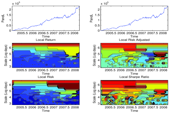
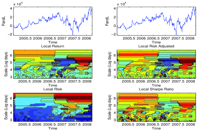
Now we consider two examples of the LRD when applied to PandL time series generated by different strategies. In particular, the first time series, Fig. 1 (top), shows relatively stationary performance over the period under consideration, with the exception of two “bumps” in the middle of 2007 and at the beginning of 2008. These “bumps” are highlighted as a valley and a peak in the LRD, as it can be seen in the contour plots for the LRA (Fig. 1, middle-right, $\beta=0.75$) and for the LSR (Fig. 1, bottom-right). The second time series, instead, Fig. 2 (top), is more volatile if compared to the first: we have good performances up to the end of 2006 when suddenly the system starts to lose money. However, at the end of 2007 a comeback is observed. Both LRA, (Fig. 2, middle-right, $\beta=0.75$), and LSR, (Fig. 2, bottom-right), capture this dynamics very faithfully: a deep valley followed by an high peak can be observed in the last part of the time series. The LRD framework, therefore, allows the practitioner to identify and stress easily specific periods in time as well as specific investment horizons that have been particularly significant during the life (or testing) of a trading system.

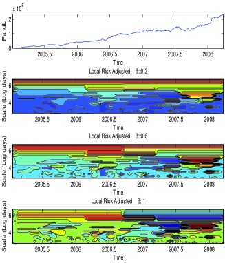
It is important to notice that LRA and LSR magnify differently the features of the time series presented in the former examples. This fact is due related to the investor’s particular appetite for risk, parameterized by $\beta$ and fixed to 0.75 in Figs. 1 and 2, that appears in the LRA. An aggressive trader would give more importance to the returns than to their fluctuations and, therefore, $\beta\approx 0$. By contrast, a risk adverse trader highlights the fluctuations, so to have $\beta\approx 1$. Examples of the LRA response to different sensitivities are shown in Fig. 3 for the first time series.

Figure 1: The two top plots are the same daily PandL generated by a certain trading strategy. The time series is shown twice in order to ease the comparison with the LRD contour plots reported underneath. On the right-hand side, we report the LRA (middle-right, $\beta=0.75$) and the LSR (bottom-right). Both representations capture the “bumps” observed in 2007 and 2008. On the left-hand side, for completeness, we show the local return, $\tilde{r}^{i}_{h}$, (middle) and the local risk, $\tilde{\sigma}^{i}_{h}$, (bottom). The contour scale goes from the dark colors for the minima to the light ones for the maxima.

Figure 2: The plots are equivalent to those in Fig. 1 but for a different trading system. The performance, in this case, starts being relatively volatile from the middle of 2006. This change in dynamics is encoded, with different emphasis, by the LRA ($\beta=0.75$) and the LSR measures.

Figure 3: Different contour plots of the LRA related to the PandL time series of Fig. 1 (top). The different values of $\beta$ (0.3, 0.6 and 1 from top to bottom) smooth or emphasize volatile periods according to the different appetite for risk chosen by the investor.

5 Extracting performance indices from the LRD

In the previous section, we introduced a framework to estimate local risk measures from the PandL of a trading strategy. The complete time/scale decomposition, despite being a faithful representation of the PandL’s dynamics, as well as visually appealing, can be cumbersome to use in practical applications, such as algorithms for strategies optimization. It is, therefore, of interest to derive a single performance indicator from the information provided by the LRD.

The advantage of having a LRD of the PandL signal lies in the possibility to “customize” the final indicator according to the user’s specific need. In other words, different traders may focus on different investment horizons or could be more interested in limited periods of time characterized by specific market condition: these preferences can be encoded in the integration of the LRD. In fact, for a generic local performance measure, $f$, (LRA or LSR, for example) we define our indicator as the convolution of this quantity with time/scale kernels over the ranges of interest as, for instance, from $T_{0}$ to $T$ for time and from $h_{min}$ to $h_{max}$ for the investment horizon. In order to ease the notation, we assume a continuous decomposition for the PandL , that is $i\rightarrow t$ and $h\rightarrow s$, and we define an LRD indicator as

$$\Phi^{f}_{\tau,\rho}=\frac{\int_{h_{min}}^{h_{max}}ds\,K_{s}(\frac{s-\rho}{\delta s})\,\eta_{f}(\tau,s)}{\int_{h_{min}}^{h_{max}}ds\,K_{s}(\frac{s-\rho}{\delta s})},$$ (7)

where

$$\eta_{f}(\tau,s)=\frac{\int_{T_{0}}^{T}dt\,K_{t}(\frac{t-\tau}{\delta t})\,f(t,s)}{\int_{T_{0}}^{T}dt\,K_{t}(\frac{t-\tau}{\delta t})},$$ (8)

being $K_{s}$ and $K_{t}$ convolution kernels, $\rho$ and $\tau$ representing the “principal” investment horizon and time while $\delta t$ and $\delta s$ are dilatation coefficients (Silverman96, ). These parameters can be tuned for different investor’s requirements, making the method particularly flexible. For example, by using hard kernels such as the Heaviside function, it is possible to cut the contribution of the performance beyond some specified look-back period. Otherwise, if it is preferred to give a weight to whole the historical performance of the trading strategy, a Gaussian kernel would be suitable.

In order to underline the flexibility of our indicator $\Phi^{f}_{\tau,\rho}$, we perform a numerical test on two artificial PandL time series for different choices of the parameters in Eqs. (7) and (8). We restrict the range of choices by fixing $\tau=\max(t)$, since investors tend to give more importance on the recent performance of their strategies. The dilatation coefficients are selected according to: $\delta s=100\rho$ and $\delta t=\left[\max(t)-\min(t)\right]/4$. The errors on the estimates have been calculated via the jacknife method (Kunsch89, ) and indicated between brackets as uncertainty in the last digit.

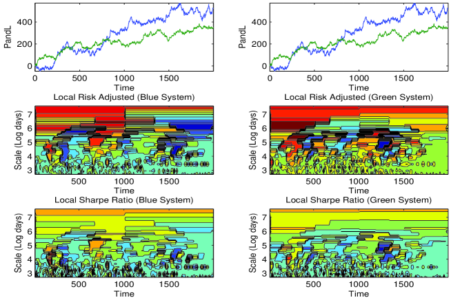
The LRD of two artificially generated PandL, each with 2000 data points, with different linear drifts as well as a different superimposed noise amplitude, is shown in Fig. 4. The first time series (blue) provides a better return at the expenses of higher volatility. The second time series (green), in contrast, exhibits a relatively stable growth. Despite the intrinsic differences, the annualized Sharpe ratio, Eq.(1), results to be the same for the two time series, namely $S=0.7(2)$, making them look equivalent from its prospective. On the other hand, the LRD framework gives a much broader picture regarding the performances of the two time series. The results are summarized in Table 1 and Table 2. In the first one, we report for different principal investment horizons, $\rho$, the values of $\Phi^{LRA}_{\tau,\rho}$ and $\Phi^{LSR}_{\tau,\rho}$ for the two trading systems when a uniform kernel is used, $K_{r}\equiv K_{t}\equiv 1$. In the second table, instead, we show the same results for Gaussian kernels. We also report the values of $\eta_{LRA}(\tau,s)$ and $\eta_{LSR}(\tau,s)$ at the scale of main interest, that is for $s\equiv\rho$. The reason behind this is that these two quantities, which are nothing but kernel weighted averages of a risk-adjusted performance, $f$, over time being the scale $s$ fixed, Eq.(8), can be considered as further performance indicator when the strategy has a characteristic time scale (holding period), $\rho$ in this case.

The results show that when we do not apply any convolution kernel, Table 1, the performance indicators $\Phi^{LRA}_{\tau,\rho}$ and $\Phi^{LSR}_{\tau,\rho}$ would pick the blue strategy, that is, the one with the highest return, as the best out of the two. However, if we consider the indicator at a specific investment horizon $\rho$, that is $\eta_{LRA}(\tau,\rho)$ and $\eta_{LSR}(\tau,\rho)$, the situation is not as clear. On the other hand, when the indicators are extracted via two Gaussian kernels centered in the last day of trade and at the horizon $\rho$, explicitly giving more importance to a particular time/scale region, the best performing system would be the green one. This result is due to the fact that the blue strategy is not performing well in the last period of the PandL series where the time kernel is centered. This simple example highlights the flexibility of the LRD framework when compared to global quantities such as the Sharpe ratio which ignore the dynamics of the performance.

Figure 4: LRD for two simulated PandL . The left hand side corresponds to the blue time series and the right hand side to the green. The noise amplitude for the blue time series is 1.5 times the green one. The Sharpe ratio, calculated via Eq. (1) is 0.7(2) for both time series and, therefore, they are undistinguishable according to this performance indicator. For the LRA we used $\beta=0.75$.

The values for $\Phi^{LRA}_{\tau,\rho}$ and $\Phi^{LSR}_{\tau,\rho}$ along with $\eta_{LRA}(\tau,\rho)$ and $\eta_{LSR}(\tau,\rho)$ for different $\rho$. The values on the left refer to the first time series (blue) in Fig. 4, while the values on the right refer to the second time series (green). The kernel used for the integration of Eq. (7) is uniform with $K_{r}\equiv K_{t}\equiv 1$. The LRA has been normalized by its standard deviation over the time/scale boxes. This procedure is not fundamental for asserting the performances of a strategy. In brackets is the error of the last digit calculated via the jacknife method. $\rho=50$ $\rho=100$ $\rho=250$ $\rho=500$ $\rho=1000$ $\Phi^{LRA}_{\tau,\rho}$00 $0.36(1)/0.34(1)$ $0.36(1)/0.34(1)$ $0.364(9)/0.34(1)$ $0.36(1)/0.34(1)$ $0.36(1)/0.34(1)$ $\Phi^{LSR}_{\tau,\rho}$00 $2.71(7)/2.4(1)$ $2.71(8)/2.4(1)$ $2.7(1)/2.37(9)$ $2.71(6)/2.37(9)$ $2.7(1)/2.4(9)$ $\eta_{LRA}(\tau,\rho)$0 $0.018(6)/0.02(1)$ $0.040(4)/0.04(1)$ $0.05(1)/0.097(9)$ $0.23(1)/0.33(2)$ $0.42(2)/0.51(2)$ $\eta_{LSR}(\tau,\rho)$0 $0.5(2)/0.5(2)$ $0.64(8)/0.6(2)$ $0.5(1)/0.9(2)$ $1.53(9)/2.2(2)$ $2.19(6)/2.6(1)$

Same as Table 1 but using two Gaussian kernels in Eqs. (7)-(8). For the calculation, $\tau=\max(t)$ while $\delta s=100\rho$, and $\delta t=\left[\max(t)-\min(t)\right]/4$. $\rho=50$ $\rho=100$ $\rho=250$ $\rho=500$ $\rho=1000$ $\Phi^{LRA}_{\tau,\rho}$00 $-0.12(2)/0.21(2)$ $-0.12(2)/0.21(4)$ $-0.11(2)/0.21(4)$ $-0.11(1)/0.22(4)$ $-0.11(2)/0.22(3)$ $\Phi^{LSR}_{\tau,\rho}$00 $1.60(6)/1.9(1)$ $1.63(6)/1.9(2)$ $1.64(5)/1.9(1)$ $1.64(4)/1.9(1)$ $1.64(8)/1.9(1)$ $\eta_{LRA}(\tau,\rho)$0 $0.00(2)/0.017(9)$ $-0.12(3)/-0.03(3)$ $0.13(7)/-0.02(7)$ $-0.58(3)/0.2(1)$ $0.02(5)/0.43(2)$ $\eta_{LSR}(\tau,\rho)$0 $0.4(1)/0.3(1)$ $-0.1(2)/0.2(3)$ $0.1(1)/0.6(1)$ $0.1(1)/2.5(3)$ $1.72(9)/2.5(1)$

As for more traditional indicators, the LDR framework can be used in the contest of investment optimization. In high-frequency trading, for example, a typical problem could be how to distribute the capital allocation among several different independent trading strategies applied over the same contract. In this case the weight vector is determined via an optimization procedure of one or more of the risk-adjusted measures, the target variables, estimated from the PandL curves obtained in the backtesting. In this contest, the use of the LRD as target variable can be interpreted as a “weighted” optimization where more emphasis can be placed, for example, on the last performance period and on a characteristic time scale associated with the strategies in question. For some more detailed discussions on trading strategies optimization in the high-frequency space, which goes beyond the scope of this work, the interested reader can refer to (Chan09, ; Aldridge10, ).

6 Discussion and conclusions

In the present paper we have introduced a local risk decomposition framework that retains dynamical information about the performance of a trading strategy. This framework is very useful for practitioners who work at high-frequencies as it provides a map of the non-stationarity and multiscale features of the PandL time series. Moreover, from the LRD it is possible to construct a single indicator for the performance of the trading system, as shown in Sec. 5. The advantage of this indicator when compared to more traditional ones, such as the Sharpe ratio for example, lies in the fact that the user can choose to put more emphasis on some period in time or some specific investment horizons according to his/her preference. It is also important to stress the local detrending procedure in the risk estimate which we have used in order to take into account for the possible non-stationarity of the time series.

On the other hand, in order to have a reliable estimation of the dynamics at different scales, the LRD requires a reasonable amount of samples in the PandL. This drawback makes the LRD more suitable for high/medium frequency trading systems rather than log term ones.

In conclusion, the LRD framework can be a useful alternative to more traditional risk-adjusted performance indicators and, consequently, it can be applied to optimization problems such as the creation of a portfolio of different high-frequency trading systems.

References

- [1] Irene Aldridge. High-frequency trading: a practical guide to algorithmic strategies and trading systems. Wiley & Sons, New Jersey, 2010.
- [2] Roy E. Bailey. The economics of financial markets. Cambridge University Press, Cambridge, UK, 2005.
- [3] Marco Bartolozzi, Derek B. Leinweber, and Anthony W. Thomas. Scale-free avalanche dynamics in the stock market. Physica A, 370:132–139, 2006.
- [4] Marco Bartolozzi, Christopher Mellen, Francis Chan, David Oliver, Tiziana Di Matteo, and Tomaso Aste. Applications of physical methods in high-frequency futures markets. Proc. of SPIE, 6802:680203, 2007.
- [5] Marco Bartolozzi, Christopher Mellen, Tiziana Di Matteo, and Tomaso Aste. Multi-scale correlations in different futures markets. The European Physical Journal B, 58(2):207–220, 2007.
- [6] J.-P. Bouchaud and M. Potters. Theory of financial risk. Cambridge University Press, Cambridge, 1999.
- [7] Ernest P. Chan. Quantitative Trading. Wiley & Sons, New Jersey, 2009.
- [8] Liu Y.H. Cizeau, P. and, M. Meyer, K.C. Peng, and H.E. Stanley. Volatility distribution in the s&p stock index. Physica A, 245:441–445, 1997.
- [9] R.L. Costa and G.L. Vasconcelos. Long-range correlations and nonstationarity in the brazilian stock market. Physica A, 329:231–248, 2003.
- [10] Michael M. Dacorogna, Ramazan Gençay, Ulrich Müller, Richard B. Olsen, and Olivier V. Pictet. An introduction to high-frequency finance. Academic Press, San Diego, 2001.
- [11] Kevin Dowd. Adjusting for risk: an improved sharpe ratio. International Review of Economics and Finance, 9:209–222, 2004.
- [12] Z. Eisler and J. Kertsz. Liquidity and the multiscaling properties of the volume traded on the stock market. Europhys. Lett., 77:28001, 2007.
- [13] P. Gopikrishnan, V. Plerou, X. Gabaix, L.A.N. Amaral, and H.E. Stanley. Price fluctuations and market activity. Physica A, 299:137–143, 2001.
- [14] P. Gopikrishnan, V. Plerou, Y.H. Liu, Gabaix X. Amaral, L.A.N. and, and H.E. Stanley. Scaling and correlation in financial time series. Physica A, 287:362–373, 2000.
- [15] D. Grech and Z. Mazur. Can one make any crash prediction in finance using the local hurst exponent idea? Physica A, 336:113–145, 2004.
- [16] Plamen Ch. Ivanov, Ainslie Yuen, Boris Podobnik, and Youngki Lee. Common scaling patterns in intertrade times of u.s. stocks. Phys. Rev. E, 69:56107, 2004.
- [17] I.M. Jnosi, B. Janecsk, and I. Kondor. Statistical analysis of 5 s index data of the budapest stock exchange. Physica A, 269:111–124, 1999.
- [18] H. R. Kunsch. The jacknife and the bootstrap for general stationary observations. The Annals of Statistics, 17:1217–1241, 1989.
- [19] Oliver Ledoit and Michael Wolf. Robust performance hypotesis testing with the sharpe ratio. Journal of Empirical Finance, 15:850–859, 2008.
- [20] Y.H. Liu, P. Cizeau, M. Meyer, K.C. Peng, and H.E. Stanley. Scaling behavior in economic time series. Physica A, 245:437–440, 1997.
- [21] Y.H. Liu, P. Gopikrishnan, P. Cizeau, M. Meyer, K.C. Peng, and H.E. Stanley. The statistical properties of the volatility price fluctuations. Phys. Rev. E, 60:1390–1400, 1990.
- [22] K. Matia, L.A.N. Amaral, S.P. Goodwin, and H.E. Stanley. Different scaling behaviors of commodity spot and future prices. Phys. Rev. E, 66:045103(R), 2002.
- [23] Attilio Meucci. Risk and Asset Allocation (third edition). Springer, Berlin, 2007.
- [24] D. Mukherjee and A. Ullah. Nonparametric sharpe ratio. Journal of Quantitative Economics, 2(2):172–185, 2004.
- [25] S.V. Muniandy, S.C. Lim, and R. Murugan. Inhomogeneous scaling behaviors in malaysian foreign currency exchange rates. Physica A, 301:407–428, 2001.
- [26] C.-K. Peng, S. V. Buldyrev, S. Havlin, M. Simons, H. E. Stanley, and A. L. Goldberger. Mosaic organization of DNA nucleotides. Physical Review E, 49(2):1685–1689, Feb 1994.
- [27] W.F. Sharpe. The sharpe ratio. Journal of Portfolio Managment, 21:49–59, 1994.
- [28] B.W. Silverman. Density estimation for statistics and data analysis. Chapman-Hall, London, 1996.
- [29] Didier Sornette. Critical phenomena in natural sciences. Springer-Verlag, Berlin, 2004.
- [30] N. Vandewalle and M. Ausloos. Coherent and random sequences in financial fluctuations. Physica A, 246:454–459, 1997.
- [31] Johannes Voit. The Statistical Mechanics of Financial Markets. Spriger-Verlag, Berlin, 2005.
- [32] Peter Woehrmann, Willy Semmler, and Martin Lettau. Nonparametric estimation of time-varying sharpe ratio in dynamic asset pricing models. Working paper 225, Institute for Empirical Research in Economics University of Zurich, 2005.