Eccentricity fluctuation effects on elliptic flow in relativistic heavy ion collisions

Abstract

We study effects of eccentricity fluctuations on the elliptic flow coefficient $v_{2}$ at mid-rapidity in both Au+Au and Cu+Cu collisions at $\sqrt{s_{NN}}=200$ GeV by using a hybrid model that combines ideal hydrodynamics for space-time evolution of the quark gluon plasma phase and a hadronic transport model for the hadronic matter. For initial conditions in hydrodynamic simulations, both the Glauber model and the color glass condensate model are employed to demonstrate the effect of initial eccentricity fluctuations originating from the nucleon position inside a colliding nucleus. The effect of eccentricity fluctuations is modest in semicentral Au+Au collisions, but significantly enhances $v_{2}$ in Cu+Cu collisions.

I Introduction

One of the major discoveries at Relativistic Heavy Ion Collider (RHIC) in Brookhaven National Laboratory (BNL) is that azimuthally anisotropic flow (the so-called elliptic flow) Ollitrault is found to be as large as an ideal hydrodynamic prediction for the first time in relativistic heavy ion collisions STARv2 ; PHENIXv2 ; reviews . Whether local thermalization, which is demanded in application of hydrodynamics, is reached is not known a priori in relativistic heavy ion collisions. Therefore the discovery indicates that the heavy ion reactions at relativistic energies provide a unique opportunity to investigate the high temperature QCD matter in equilibrium. The discovery also indicates a new possibility to obtain the transport properties of the QCD matter under extreme conditions. Effects of viscosity have already been taken into account in several hydrodynamic simulations Song ; Chaudhuri ; Baier ; Dusling ; Denicol and also specifically in distortion of distribution functions Teaney ; Monnai to calculate elliptic flow coefficients.

Systematic studies showed, however, that the reasonable agreement between results from ideal hydrodynamics and elliptic flow data has been achieved only by a particular combination of dynamical modeling, namely initial conditions from the Glauber model, the perfect fluid quark gluon plasma (QGP) core, and the dissipative hadronic corona HG05 . For example, when one takes initial conditions from the color glass condensate (CGC) model instead of the conventional Glauber model ones, the result overshoots the elliptic flow data HHKLN due to initial eccentricity larger than that from the Glauber model Kuhlman:2006qp . Even within the Glauber model initializations, the agreement between hydrodynamic results and the data, in particular centrality dependence of the elliptic flow, is not perfect, which would be due to an absence of initial fluctuation effects MS03 ; Zhu:2005qa ; Bhalerao:2006tp ; phobosfluc ; Andrade:2006yh ; Drescher:2006ca ; Broniowski:2007ft ; Broniowski:2007nz ; Voloshin:2007pc . Therefore, further investigation is indispensable toward better understanding of the elliptic flow data and, in turn, understanding of transport properties of the QGP.

In this paper, we follow up with the previous study HHKLN ; HHKLN2 based on an ideal hydrodynamic description of the QGP fluid and a microscopic description of the hadronic gas by taking into account the initial eccentricity fluctuation effects. It was found that large initial eccentricity in some particular modeling of the CGC picture is attributed to improper treatment of nuclear edge regions to define the saturation scale Drescher:2006ca . Improved treatment of the edge leads to slight reduction of eccentricity Drescher:2006ca . So it would be interesting to see whether the improved CGC model ends up with reproduction of elliptic flow data as well as how initial fluctuation of eccentricity affects elliptic flow coefficients in both the Glauber model and the CGC model.

This paper is organized as follows. In Sec. II, we first overview the dynamical modeling of relativistic heavy ion collisions based on a hybrid (hydro+cascade) approach. We discuss how to implement the eccentricity fluctuation in the hydrodynamic initial conditions. For the initial transverse profiles, we employ the Glauber model and the CGC model and compare the eccentricities with each other. In Sec. III, we investigate the effect of eccentricity fluctuation on the elliptic flow coefficients by using the hybrid dynamical model. Section IV is devoted to conclusion.

II The model

II.1 Dynamical modeling of heavy ion collisions

Our study is mainly based on a hybrid model which combines an ideal fluid dynamical description of the QGP stage with a realistic kinetic simulation of the hadronic stage HHKLN ; HHKLN2 ; BassDumitru ; TLS01 ; NonakaBass ; Petersen:2008dd ; Werner . Relativistic hydrodynamics is the most relevant framework to understand the bulk and transport properties of the QGP since it directly connects the collective flow developed during the QGP stage with its equation of state (EOS). It is based on the key assumption of local thermalization. Since this assumption breaks down during both the very anisotropic initial matter formation stage and the dilute late hadronic rescattering stage, the hydrodynamic framework can be applied at best only during the intermediate period. To describe the breakdown of the hydrodynamic description during the late hadronic stage due to expansion and dilution of the matter, one may have two options: One can either impose a sudden transition from thermalized matter to non-interacting and free-streaming hadrons through the Cooper-Frye prescription CF at a decoupling temperature $T_{\mathrm{dec}}$, or make a transition from a macroscopic hydrodynamic description to a microscopic kinetic description at a switching temperature $T_{\mathrm{sw}}$. We here use the first approach to fix the initial parameters by comparison with the multiplicity data. After all initial parameters are fixed, we carry out hybrid simulations to investigate the effect of initial eccentricity fluctuations as well as hadronic dissipation.

For the space-time evolution of the perfect QGP fluid we solve numerically the equations of motion of ideal hydrodynamics for a given initial state in three spatial dimensions and in time Hiranov2eta :

$$\partial_{\mu}T^{\mu\nu} = 0,$$ (1)

$$T^{\mu\nu} = (e+p)u^{\mu}u^{\nu}-pg^{\mu\nu}.$$ (2)

Here $e$, $p$, and $u^{\mu}$ are energy density, pressure, and four-velocity of the fluid, respectively. We neglect the net baryon density due to its smallness at collider energies BRAHMS:stopping . We have solved Eq. (1) in $(\tau,\,x,\,y,\,\eta_{s})$ coordinates Hiranov2eta where $\bm{x}_{\perp}=(x,y)$ is a transverse coordinate, $\tau{\,=\,}\sqrt{t^{2}{-}z^{2}}$ and $\eta_{s}{\,=\,}\frac{1}{2}\ln[(t{+}z)/(t{-}z)]$ are longitudinal proper time and space-time rapidity, respectively, adequate for the description of collisions at ultra-relativistic energies. As will be discussed later in the next subsection, we calculate the initial condition only at midrapidity and neglect possible fluctuation and correlation effects in the forward/backward rapidity regions in this work. So we assume longitudinal boost invariance up to the longitudinal boundary of the mesh at $\eta_{s}=5$ in three dimensional grids and calculate the observables only at midrapidity. The solution for the positive rapidity region is properly reflected to the negative rapidity region. We have checked that there is neither rapidity dependence nor numerical artifacts from the finite volume in the longitudinal direction on the observables at midrapidity.

For the high temperature QGP phase ($T>T_{c}=170$ MeV) we use the EOS of massless parton gas ($u$, $d$, $s$ quarks and gluons) with a bag pressure $B$:

$$p=\frac{1}{3}(e-4B)$$ (3)

The bag constant is tuned to $B^{\frac{1}{4}}=247.19$ MeV to ensure a first order phase transition to a hadron resonance gas at critical temperature $T_{c}=170$ MeV. The hadron resonance gas model at $T<T_{c}$ includes all hadrons up to the mass of the $\Delta(1232)$ resonance. Our hadron resonance gas EOS implements chemical freeze-out at $T_{\mathrm{chem}}{{\,=\,}}T_{c}=170$ MeV HT02 . This is achieved by introducing appropriate temperature-dependent chemical potentials $\mu_{i}(T)$ for each hadronic species $i$ HT02 ; Bebie ; spherio ; Teaney:2002aj ; Kolb:2002ve ; Huovinen:2007xh . In our hybrid model simulations we switch from ideal hydrodynamics to a hadronic cascade model at the switching temperature $T_{\mathrm{sw}}=169$ MeV. The subsequent hadronic rescattering cascade is modeled by JAM jam , initialized with hadrons distributed according to the hydrodynamic model output and calculated with the Cooper-Frye formula CF along the $T_{\mathrm{sw}}{\,=\,}169$ MeV hypersurface rejecting inward-going particles.

II.2 Initial conditions with eccentricity fluctuation effects

The space-time evolution of thermodynamic variables is described in the hydrodynamic framework. The concept of ensemble average in a sense of statistical mechanics is implicitly there to interpret the thermodynamic variables. So we identify the ensemble with a large number of collision events and suppose the hydrodynamic solution represents an average behavior of the space-time evolution of the matter for a given centrality cut. This is contrary to an approach in Refs. Andrade:2006yh ; Andrade:2008xh in which hydrodynamic equations with lumpy initial conditions are solved in an event-by-event basis. The smooth initial condition is, however, required in some practical reasons in our approach. Such a lumpy initial condition could generate sizable numerical viscosity in hydrodynamic simulations if the mesh size is not sufficiently small. In the present study, the mesh size in the transverse direction is $\Delta x=0.3$ (0.2) fm in Au+Au (Cu+Cu) collisions. The mesh size is of the same order of the transverse size of nucleons, so it would be hard to capture possible lumpy structures in the initial conditions. Moreover, one needs to perform a large number of simulations to gain sufficient statistics in final observables. Therefore we pursue a more conservative approach by initializing the distribution of thermodynamic variables with smooth functions averaged over many events.

For initial conditions in this study, we employ the Monte-Carlo version of both the Glauber model and the factorized Kharzeev-Levin-Nardi (fKLN) model Drescher:2006ca to generate the initial distribution of entropy density in an event-by-event basis. One has extensively used the Monte Carlo Glauber model (MC-Glauber) to determine the centrality cut, the average numbers of participants and binary collisions for a given centrality, and so on Miller:2007ri . On the other hand, the fKLN model enables us to improve the treatment of entropy production processes. This model also gives a natural description near the edge regions compared to the ordinary KLN approach KLN01 employed by us previously Hirano:2004rs . The Monte-Carlo version of fKLN, which we call MC-KLN, implements the fluctuations of gluon distribution due to the position of hard sources (nucleons) in the transverse plane Drescher:2006ca .

We first calculate a transverse entropy density profile

$$s_{0}(\bm{x}_{\perp})=s(\tau=\tau_{0},x,y,\eta_{s}=0)$$ (4)

in each sample at an impact parameter $b$ for a given centrality, where $\tau_{0}=0.6$ fm/$c$ is the initial time for the hydrodynamical simulations. Then the variances of the profile are obtained from

$$\sigma_{x}^{2} = \langle x^{2}\rangle-\langle x\rangle^{2},$$ (5)

$$\sigma_{y}^{2} = \langle y^{2}\rangle-\langle y\rangle^{2},$$ (6)

$$\sigma_{xy} = \langle xy\rangle-\langle x\rangle\langle y\rangle.$$ (7)

Here $\langle\cdots\rangle$ describes the average over transverse plane by weighting the entropy density in a single sample:

$$\langle\cdots\rangle=\frac{\int d^{2}x_{\perp}\cdots s_{0}(\bm{x}_{\perp})}{\int d^{2}x_{\perp}s_{0}(\bm{x}_{\perp})}.$$ (8)

The eccentricity with respect to reaction plane, the participant eccentricity, and the corresponding transverse areas can be defined phobosfluc , respectively, as

$$\varepsilon_{\mathrm{RP}} = \frac{\sigma_{y}^{2}-\sigma_{x}^{2}}{\sigma_{y}^{2}+\sigma_{x}^{2}},$$ (9)

$$\varepsilon_{\mathrm{part}} = \frac{\sqrt{(\sigma_{y}^{2}-\sigma_{x}^{2})^{2}+4\sigma_{xy}^{2}}}{\sigma_{y}^{2}+\sigma_{x}^{2}},$$ (10)

$$S_{\mathrm{RP}} = \pi\sqrt{\sigma_{x}^{2}\sigma_{y}^{2}},$$ (11)

$$S_{\mathrm{part}} = \pi\sqrt{\sigma_{x}^{2}\sigma_{y}^{2}-\sigma_{xy}^{2}}.$$ (12)

It should be noted here that, in calculating eccentricity and transverse area, we use the entropy density profile instead of the distribution of participants. Thus the eccentricity depends on modeling of initialization, i.e., transverse profiles in hydrodynamic simulations.

The impact parameter vector and the true reaction plane are not known experimentally. So one can set an apparent frame of created matter shifted by $(x,y)=(\langle x\rangle,\langle y\rangle)$ and tilted by $\Psi$ from the true frame in the transverse plane phobosfluc :

$$\tan 2\Psi=\frac{\sigma_{y}^{2}-\sigma_{x}^{2}}{2\sigma_{xy}}.$$ (13)

The anisotropy of particle distribution could be correlated with the misidentified frame. To take account of this, we first shift the center-of-mass of the system to the origin in the calculation frame and then rotate the profile in the azimuthal direction by $\Psi$ to match the apparent reaction plane to the true reaction plane. We generate the next sample of an entropy density profile again as above and average the profiles over many samples. We repeat the above procedure for many samples until the initial distribution is smooth enough. The initial conditions obtained in this way contain the effects of eccentricity fluctuation even though the profile is smooth. In particular, even in case of vanishing impact parameter, eccentricity is finite due to its event-by-event fluctuation. It is the particle distribution calculated from the initial conditions mentioned above that can be directly compared with the experimental data. Note that the procedure averaging over many samples without shift or rotation corresponds to conventional initialization without the effect of eccentricity fluctuation.

II.3 Monte Carlo Glauber model

In the Monte Carlo version of the Glauber model, we first sample the positions of nucleons according to a nuclear density distribution for two colliding nuclei. A nucleon-nucleon collision takes place if their distance $d$ in the transverse plane (orthogonal to the beam axis) satisfies the condition

$$d\leq\sqrt{\sigma_{NN}^{\text{in}}/\pi},$$ (14)

where $\sigma_{NN}^{\text{in}}=41.94$ mb is the inelastic nucleon-nucleon cross section at $\sqrt{s_{NN}}=200$ GeV. The number of binary collisions $N_{\mathrm{coll}}$ is obtained by counting total number of nucleon-nucleon collisions, and the number of participants $N_{\mathrm{part}}$ is the total number of nucleons which collide at least once.

In the ordinary MC-Glauber model, the following Woods-Saxon distribution is employed as a nuclear density profile

$$\rho_{\mathrm{WS}} = \frac{\rho_{0}}{\exp\left(\frac{r-r_{0}}{d}\right)+1},$$ (15)

where $\rho_{0}=$ 0.1695 (0.1686) fm^-3, $r_{0}=$ 6.38 (4.20641) fm, $d=$ 0.535 (0.5977) fm for a gold (copper) nucleus Miller:2007ri ; De Jager:1987qc . If one assumes a profile of nucleon as the delta function, the resulting nuclear density is nothing but the Woods-Saxon distribution

$$\rho(\vec{x})=\int\delta^{(3)}(\vec{x}-\vec{x}_{0})\rho_{\mathrm{WS}}(\vec{x}_{0})d^{3}\vec{x}_{0}.$$ (16)

However, in the case of finite size profile for nucleons as assumed in the MC-Glauber model, the nuclear density is no longer the same as the Woods-Saxon distribution.

$$\rho(\vec{x}) = \int\Delta(\vec{x}-\vec{x}_{0})\rho_{\mathrm{WS}}(\vec{x}_{0})d^{3}\vec{x}_{0},$$ (17)

$$\Delta(\vec{x}-\vec{x}_{0}) = \frac{\theta(r_{N}-\mid\vec{x}-\vec{x}_{0}\mid)}{V_{N}},$$ (18)

$$V_{N} = \frac{4\pi r_{N}^{3}}{3},\quad r_{N}=\sqrt{\frac{\sigma_{NN}^{\mathrm{in}}}{\pi}}.$$ (19)

This is illustrated in Fig. 1.

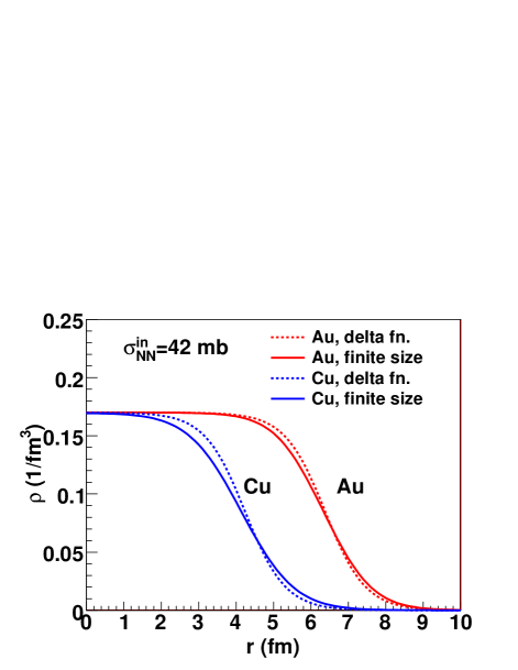
Figure 1: (Color online) Nuclear density as a function of nuclear radius. Solid lines show nuclear density distribution for gold and copper nuclei in which a finite nucleon profile is implemented and positions of nucleons are sampled according to the Woods-Saxon distribution with default parameter sets. Dashed lines show the Woods-Saxon distribution with default parameter sets.

Obviously, nuclear surface is more diffused in both gold and copper nuclei due to the finite nucleon profile in Eq. (18). As a matter of fact, eccentricity becomes smaller by $\sim 10\%$ Drescher:2006ca unless one adjusts the Woods-Saxon parameters according to the finite nucleon profile. So we parameterize the distribution of nucleon positions to reproduce the Woods-Saxon distribution with default parameters in Eq. (15) Broniowski:2007nz . In our MC-Glauber model, we find the default Woods-Saxon distribution is reproduced by a larger radius parameter $r_{0}=$ 6.42 (4.28) fm and a smaller diffuseness parameter $d=$ 0.44 (0.50) fm (i.e., sharper boundary of a nucleus) for a gold (copper) nucleus than the default parameters. This kind of effect exists almost all Monte Carlo approaches of the collisions including event generators. If one wants to discuss eccentricity and elliptic flow coefficient $v_{2}$ within $\sim 10\%$ accuracy, this effect should be taken into account.

We assume that the initial entropy profile in the transverse plane at midrapidity is proportional to a linear combination of the number density of participants and that of binary collisions in the Glauber model

$$s_{0}(\bm{x}_{\perp}) = \left.\frac{dS}{\tau_{0}dxdyd\eta_{s}}\right|_{\eta_{s}=0}$$ (20)

$$= \frac{C}{\tau_{0}}\left(\frac{1-\delta}{2}\frac{dN_{\mathrm{part}}}{d^{2}x_{\perp}}+\delta\frac{dN_{\mathrm{coll}}}{d^{2}x_{\perp}}\right).$$

Parameters $C=19.8$ and $\delta=0.14$ have been fixed through comparison with the centrality dependence of multiplicity data in Au+Au collisions at RHIC PHOBOS_Nch by pure hydrodynamic calculations with $T_{\mathrm{dec}}=100$ MeV. Notice that the total multiplicity of the produced particle does not change during the late hadronic stage due to the chemical freezeout in the EOS.

II.4 Monte Carlo KLN model

In the MC-KLN model, the saturation scale for a nucleus $A$ at a transverse coordinate $\bm{x}_{\perp}$ in each sample is given by

$$Q_{s,A}^{2}(x;\bm{x}_{\perp}) = Q_{s,0}^{2}\frac{T_{A}(\bm{x}_{\perp})}{T_{A,0}}\left(\frac{x_{0}}{x}\right)^{\lambda}$$ (21)

and similarly for a nucleus $B$. Here, parameters $Q_{s,0}^{2}=2$ GeV², $T_{A,0}=1.53$ fm^-2, $x_{0}=0.01$, and $\lambda=0.28$ are used. Thickness function at each transverse coordinate is obtained by counting the number of wounded nucleons $N$ within a tube extending in the beam direction with radius $r=\sqrt{\sigma_{NN}^{\text{in}}/\pi}$ from each grid point:

$$T_{A}(\bm{x}_{\perp})=\frac{N}{\sigma_{NN}^{\text{in}}}.$$ (22)

For each generated configuration of nucleons in colliding nuclei, the $k_{T}$-factorization formula is applied at each transverse coordinate to obtain the distribution of produced gluons locally. We apply the Kharzeev-Levin-Nardi (KLN) approach KLN01 in the version previously employed in Hirano:2004rs . In this approach, the distribution of gluons at each transverse coordinate $\bm{x}_{\perp}$ produced with rapidity $y$ is given by the $k_{T}$-factorization formula GLR83

$$\frac{dN_{g}}{d^{2}x_{\perp}dy} = \frac{2\pi^{2}}{C_{F}}\int\frac{d^{2}p_{T}}{p_{T}^{2}}\int^{p_{T}}\frac{d^{2}k_{T}}{4}\alpha_{s}(Q^{2})$$ (23)

$$\times \phi_{A}(x_{1},(\bm{p}_{T}{+}\bm{k}_{T})^{2}/4;\bm{x}_{\perp})$$

$$\times \phi_{B}(x_{2},(\bm{p}_{T}{-}\bm{k}_{T})^{2}/4;\bm{x}_{\perp}),$$

where $x_{1,2}{{\,=\,}}p_{T}\exp(\pm y)/\sqrt{s}$ and $p_{T}$ is the transverse momentum of the produced gluons. We choose an upper limit of 10 GeV/$c$ for the $p_{T}$ integration. For the unintegrated gluon distribution function we use

$$\phi_{A}(x,k^{2}_{T};\bm{x}_{\perp})=\frac{\kappa C_{F}}{2\pi^{3}}\frac{(1-x)^{4}}{\alpha_{s}(Q_{s}^{2})}\frac{Q_{s}^{2}}{\max(Q_{s}^{2},k^{2}_{T})},$$ (24)

where $C_{F}=(N_{c}^{2}-1)/(2N_{c})$. The parameter $\kappa^{2}=1.75$ is chosen for the overall normalization of the gluon multiplicity in order to fit the multiplicity data in Au+Au collisions at RHIC PHOBOS_Nch .

As an initial condition for hydrodynamical calculations, the initial entropy density in the transverse plane is obtained by

$$s_{0}(\bm{x}_{\perp}) = 3.6n_{g}$$ (25)

$$= 3.6\left.\frac{dN_{g}}{\tau_{0}d^{2}x_{\perp}d\eta_{s}}\right|_{y=\eta_{s}=0}.$$

Here we identify gluon’s momentum rapidity $y$ with space-time rapidity $\eta_{s}$.

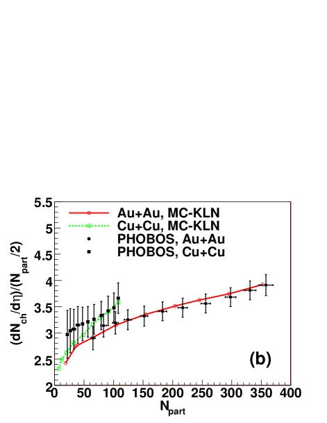
Figure 2: (Color online) Centrality dependences of charged particle multiplicity in Au+Au (solid line) and Cu+Cu (dashed line) collisions at $\sqrt{s_{NN}}=200$ GeV. (a) Initial conditions taken from the MC-Glauber model. (b) Initial conditions taken from the MC-KLN model. Experimental data are from Refs. PHOBOS_Nch ; Alver:2008ck .

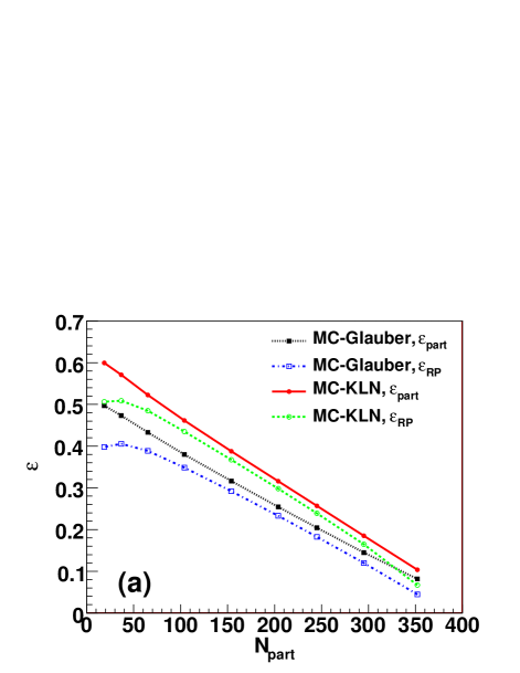
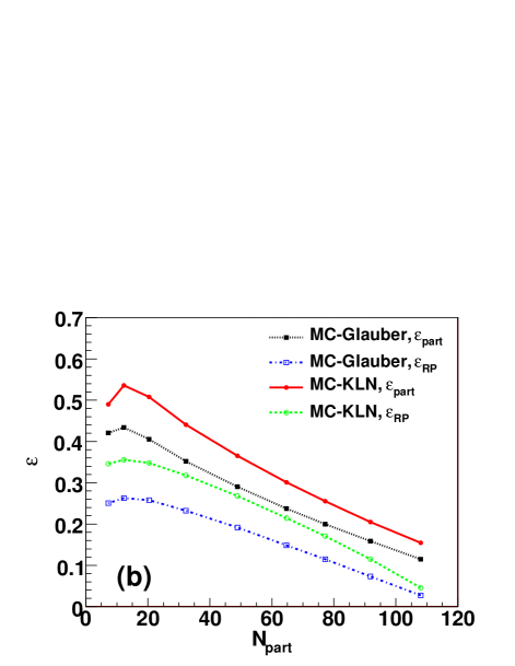
Figure 3: (Color online) Eccentricity as a function of $N_{\mathrm{part}}$ in (a) Au+Au and (b) Cu+Cu collisions. Solid, dotted, dashed, and dash-dotted lines correspond to $\varepsilon_{\mathrm{part}}$ from the MC-KLN model, $\varepsilon_{\mathrm{part}}$ from the MC-Glauber model, $\varepsilon_{\mathrm{RP}}$ from the MC-KLN model, and $\varepsilon_{\mathrm{RP}}$ from the MC-Glauber model, respectively.

III Results

III.1 Centrality dependence of multiplicity

Centrality dependences of multiplicity in the MC-Glauber model are compared with the PHOBOS data PHOBOS_Nch ; Alver:2008ck in Fig. 2 (a). Centrality dependence in Au+Au collisions is well reproduced with a two component (soft + hard) model with a small fraction of hard component $\delta=0.14$. The MC-KLN model with the setting mentioned in the previous section also gives a reasonable agreement with the data as shown in Fig. 2 (b). We did not tune initial parameters in Cu+Cu collisions. The multiplicity in the Glauber model depends only on $N_{\mathrm{part}}$ regardless of the collision system, while a non-trivial $N_{\mathrm{part}}$ dependence appears in the MC-KLN model: At a fixed $N_{\mathrm{part}}$, $(dN_{\mathrm{ch}}/d\eta)/(N_{\mathrm{part}}/2)$ in Cu+Cu collisions is larger than the one in Au+Au collisions. All results are obtained by solving the hydrodynamic equations below to $T_{\mathrm{dec}}=100$ MeV. In the actual calculations of elliptic flow coefficients, we replace the hadronic fluids with the hadronic gases utilizing a hadronic cascade model. Nevertheless, the centrality dependence of the multiplicity is still within error bars HHKLN3 .

III.2 Eccentricity

The eccentricities as functions of $N_{\mathrm{part}}$ with or without eccentricity fluctuations are compared in the MC-Glauber and MC-KLN models in Au+Au (Fig. 3 (a)) and Cu+Cu (Fig. 3 (b)) collisions. The impact parameter range, the number of participants, the eccentricity, and the transverse area are summarized in Appendix A for each centrality from 0-5% to 60-70% in Au+Au (Table 1) and Cu+Cu (Table 2) collisions at $\sqrt{s_{NN}}=200$ GeV. In semicentral Au+Au collisions (10-50% centrality), the effect of initial fluctuations enhances eccentricity parameter by 8-11% (5-8%) in the MC-Glauber (MC-KLN) model. The enhancement factor $\varepsilon_{\mathrm{part}}/\varepsilon_{\mathrm{RP}}$ is the largest at the very central bin (0-5% centrality): $\varepsilon_{\mathrm{part}}/\varepsilon_{\mathrm{RP}}=$ 1.83 in the MC-Glauber model and 1.53 in the MC-KLN model. A qualitatively similar behavior is observed in Cu+Cu collisions as shown in Fig. 3 (b). However, it is quantitatively different: the enhancement factor is 1.51-1.74 (1.36-1.50) in the MC-Glauber (MC-KLN) model in semicentral collisions (10-50% centrality). In the very central events (0-5% centrality), the factor reaches 4.20 (3.36) in the MC-Glauber (MC-KLN) model. Thus the resultant elliptic flow coefficient is expected to be enhanced by almost the same amount of the factor due to eccentricity fluctuations especially in Cu+Cu collisions. We will demonstrate it by using a dynamical model in the next subsection.

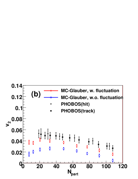
Figure 4: (Color online) Centrality dependences of $v_{2}$ for charged particles at mid-rapidity in (a) Au+Au and (b) Cu+Cu collisions at $\sqrt{s_{NN}}=200$ GeV with the MC-Glauber model initial conditions are compared with PHOBOS data (filled plots) Back:2004mh . Open circles (squares) are results with (without) eccentricity fluctuation.

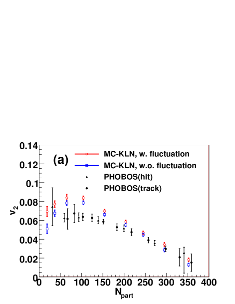
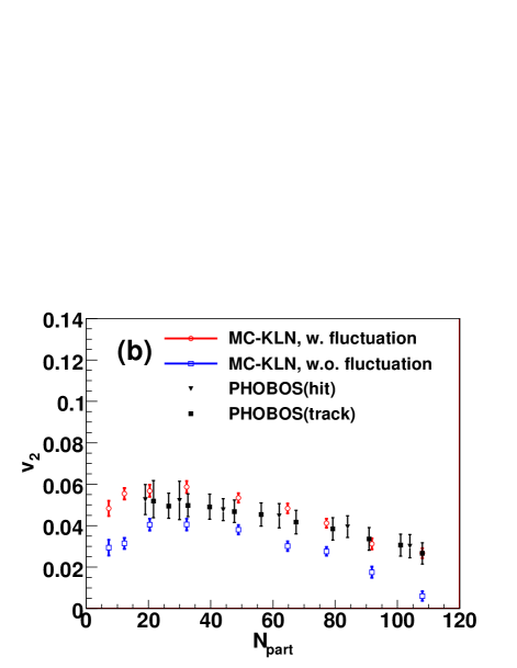
Figure 5: (Color online) Centrality dependences of $v_{2}$ for charged particles at mid-rapidity in (a) Au+Au and (b) Cu+Cu collisions at $\sqrt{s_{NN}}=200$ GeV with the MC-KLN model initial conditions are compared with PHOBOS data (filled plots) Back:2004mh . Open circles (squares) are results with (without) eccentricity fluctuation.

$\varepsilon_{\mathrm{RP}}$ in the MC-Glauber model is consistent with our previous result in which we used the standard eccentricity HHKLN . Notice that the consistency is achieved only after retuning the Woods-Saxon parameters due to finite nucleon profiles discussed in the previous section. $\varepsilon_{\mathrm{RP}}$ in the MC-KLN model is slightly smaller Drescher:2006ca than the result from the naive KLN model HHKLN . In the MC-KLN model, there exists the minimum saturation scale which is nothing but the saturation scale of a nucleon. On the other hand, the saturation scale in the naive KLN model can be arbitrary small below to $\Lambda_{\mathrm{QCD}}$, which leads to a sharper transverse profile and large eccentricity. We found eccentricity is reduced by $\sim 15\%$ in the MC-KLN model compared to the KLN model, which would affect the elliptic flow coefficients at the same amount.

III.3 Elliptic flow coefficient

Figure 4 shows the centrality dependence of $v_{2}$ for charged hadrons at mid-rapidity ($\mid\eta\mid<1$) in the Glauber model initialization in (a) Au+Au and (b) Cu+Cu collisions at $\sqrt{s_{NN}}=200$ GeV. Experimental data Back:2004mh are reasonably reproduced in Au+Au collisions. The effect of eccentricity fluctuations is not significant in Au+Au collisions, whereas $v_{2}$ is largely enhanced in Cu+Cu collisions due to fluctuation effects. These tendencies are also expected from the results of initial eccentricity as shown in Fig. 3. Interestingly elliptic flow coefficients $v_{2}$ in the Glauber model initial conditions still slightly undershoot the experimental data, in particular, in Cu+Cu collisions even with fluctuation effects.

Figure 5 is the same as Fig. 4 but the initial conditions are taken from the MC-KLN model. Again, the effect of eccentricity fluctuations is small in Au+Au collisions but is large in Cu+Cu collisions. Due to larger initial eccentricity in the MC-KLN model than the MC-Glauber model, the results are somewhat larger than the experimental data in peripheral Au+Au collisions. Whereas, we reasonably reproduce the $v_{2}$ data in Cu+Cu collisions. It should be noted that the results in Au+Au collisions lie systematically below the ones in Fig. 2 of Ref. HHKLN which employed the naive KLN model. This is due to the reduction of eccentricity by employing the fKLN model.

In both cases, the results using a more sophisticated EOS such as the one from the numerical simulations of the lattice QCD Cheng:2007jq would be demanded. The EOS from the lattice simulations has a cross-over behavior rather than the first order phase transition. Therefore it is harder in the vicinity of pseudo-critical temperature $T_{c}\sim 190$ MeV and softer in the high temperature region up to $T\sim 2T_{c}$ than the one employed in the present study. Because of the above reasons, whether final $v_{2}$ is enhanced or reduced in comparison with the current results would be non-trivial in the case of the EOS from the lattice QCD. Detailed studies on the dependences of $v_{2}$ on the EOS will be reported elsewhere.

IV Conclusions

We calculated the elliptic flow parameter as a function of the number of participants in the QGP hydro plus the hadronic cascade model and found that the effect of eccentricity fluctuations is visible in very central and peripheral Au+Au collisions and is quite large in Cu+Cu collisions. This strongly suggests that the effect of eccentricity fluctuations is an important factor which has to be included in the dynamical model for understanding of the elliptic flow data and for precise extraction of transport properties from the data.

We also found that a finite nucleon size assumed in the conventional Monte Carlo approaches reduces initial eccentricity by $\sim$10% with a default Woods-Saxon parameter set. This requires reparametrization of the nuclear radius and the diffuseness parameter to obtain the actual nuclear distribution in the case of the finite profile of nucleons as implemented in the Monte Carlo Glauber model.

In the case of the Glauber type initialization, the results still undershot the experimental data a little in both Au+Au and Cu+Cu collisions even after inclusion of eccentricity fluctuation effects. If one implemented the viscosity in the QGP phase, the results of $v_{2}$ would get reduced. So there is almost no room for the viscosity in the QGP stage to play a role in the Glauber initial conditions within the hybrid approach with the ideal gas EOS in the QGP phase.

On the other hand, we overpredicted $v_{2}$ in peripheral ($N_{\mathrm{part}}<150$) Au+Au collisions in the CGC model. Viscous effects in the QGP phase could reduce the $v_{2}$ and enable us to reproduce the data in Au+Au collisions in this case. However, the results are already comparable with the data in Cu+Cu collisions even though the number of participants is almost the same as that in peripheral Au+Au collisions. So it would be non-trivial whether the same viscous effects also give the right amount of $v_{2}$ in Cu+Cu collisions.

So far, one has been focusing on comparison of hydrodynamic results with $v_{2}$ data only in Au+Au collisions. The experimental data in Cu+Cu collisions also have a strong power to constrain the dynamical models. Therefore, simultaneous analysis of $v_{2}$ data in both Au+Au and Cu+Cu collisions will be called for in future hydrodynamic studies.

Appendix A Centrality dependence of eccentricity and transverse area

We obtain centrality in our model as follows. Using the Glauber model, one calculates centrality, namely the fraction of inelastic cross section as a function of impact parameter,

$$c(b) = \frac{2\pi\int_{0}^{b}b^{\prime}db^{\prime}\left(1-e^{-\sigma_{NN}^{\mathrm{in}}T_{AA}(b^{\prime})}\right)}{2\pi\int_{0}^{\infty}b^{\prime}db^{\prime}\left(1-e^{-\sigma_{NN}^{\mathrm{in}}T_{AA}(b^{\prime})}\right)},$$ (26)

$$T_{AA}(b) = \int d^{2}x_{\perp}T_{A}\left(x-\frac{b}{2},y\right)T_{A}\left(x+\frac{b}{2},y\right).$$

For a given range of centrality $c_{\mathrm{min}}<c<c_{\mathrm{max}}$, the maximum and minimum impact parameters can be defined from Eq. (26) as $c(b_{\mathrm{max}})=c_{\mathrm{max}}$ and $c(b_{\mathrm{min}})=c_{\mathrm{min}}$, respectively. In generating initial profiles, an impact parameter is randomly chosen in $b_{\mathrm{min}}<b<b_{\mathrm{max}}$ for each centrality bin with a probability

$$P(b)db=\frac{2b}{b_{\mathrm{max}}^{2}-b_{\mathrm{min}}^{2}}db.$$ (28)

Impact parameter ranges, the resultant number of participants, eccentricity with respect to the reaction plane, participant eccentricity, and transverse area are summarized in Table 1 for Au+Au collisions and Table 2 for Cu+Cu collisions. These parameters would be very useful to see whether $v_{2}$ data reach the so-called hydrodynamic limit or not Drescher:2007cd . It might be possible to divide all events into centralities according to the Monte Carlo results of, e.g., the $N_{\mathrm{part}}$ distribution.

Table 1: Centrality dependence of eccentricity and transverse area in Au+Au collisions.

Centrality(%)	0-5	5-10	10-15	15-20	20-30	30-40	40-50	50-60	60-70
$b_{\mathrm{min}}$ (fm)	0.0	3.3	4.7	5.8	6.7	8.2	9.4	10.6	11.6
$b_{\mathrm{max}}$ (fm)	3.3	4.7	5.8	6.7	8.2	9.4	10.6	11.6	12.5
$N_{\mathrm{part}}$	352	295	245	204	154	104	65.1	36.8	18.8
$\epsilon_{\mathrm{RP}}^{\mathrm{MC-Glauber}}$	0.0446	0.120	0.183	0.233	0.292	0.348	0.389	0.405	0.398
$\epsilon_{\mathrm{part}}^{\mathrm{MC-Glauber}}$	0.0818	0.145	0.204	0.254	0.316	0.380	0.433	0.473	0.497
$S_{\mathrm{RP}}^{\mathrm{MC-Glauber}}$ (fm2)	23.4	20.5	18.0	16.0	13.5	10.9	8.69	6.78	5.07
$S_{\mathrm{part}}^{\mathrm{MC-Glauber}}$ (fm2)	23.4	20.5	18.0	16.0	13.5	10.9	8.65	6.73	5.05
$\epsilon_{\mathrm{RP}}^{\mathrm{MC-KLN}}$	0.0671	0.165	0.239	0.298	0.367	0.435	0.485	0.509	0.506
$\epsilon_{\mathrm{part}}^{\mathrm{MC-KLN}}$	0.103	0.185	0.257	0.316	0.387	0.461	0.522	0.571	0.599
$S_{\mathrm{RP}}^{\mathrm{MC-KLN}}$ (fm2)	23.8	20.1	17.3	15.1	12.4	9.67	7.42	5.55	3.96
$S_{\mathrm{part}}^{\mathrm{MC-KLN}}$ (fm2)	23.7	20.1	17.2	15.0	12.3	9.55	7.26	5.33	3.67

Table 2: Centrality dependence of eccentricity and transverse area in Cu+Cu collisions.

Centrality(%)	0-5	5-10	10-15	15-20	20-30	30-40	40-50	50-60	60-70
$b_{\mathrm{min}}$ (fm)	0.0	2.4	3.3	4.1	4.7	5.8	6.7	7.5	8.2
$b_{\mathrm{max}}$ (fm)	2.4	3.3	4.1	4.7	5.8	6.7	7.5	8.2	8.9
$N_{\mathrm{part}}$	108	91.8	77.2	64.7	48.9	32.3	20.4	12.3	7.27
$\epsilon_{\mathrm{RP}}^{\mathrm{MC-Glauber}}$	0.0274	0.0733	0.115	0.148	0.192	0.232	0.257	0.263	0.251
$\epsilon_{\mathrm{part}}^{\mathrm{MC-Glauber}}$	0.115	0.159	0.200	0.237	0.290	0.352	0.406	0.434	0.421
$S_{\mathrm{RP}}^{\mathrm{MC-Glauber}}$ (fm2)	12.1	11.0	10.1	9.15	7.98	6.57	5.32	4.12	3.00
$S_{\mathrm{part}}^{\mathrm{MC-Glauber}}$ (fm2)	12.1	11.0	10.0	9.12	7.94	6.54	5.30	4.14	3.11
$\epsilon_{\mathrm{RP}}^{\mathrm{MC-KLN}}$	0.0457	0.115	0.171	0.214	0.268	0.318	0.348	0.356	0.346
$\epsilon_{\mathrm{part}}^{\mathrm{MC-KLN}}$	0.154	0.205	0.256	0.301	0.365	0.441	0.508	0.536	0.490
$S_{\mathrm{RP}}^{\mathrm{MC-KLN}}$ (fm2)	11.7	10.3	9.18	8.18	6.96	5.54	4.33	3.20	2.16
$S_{\mathrm{part}}^{\mathrm{MC-KLN}}$ (fm2)	11.6	10.2	9.06	8.04	6.78	5.31	4.04	2.88	1.89

References

- (1) J. Y. Ollitrault, Phys. Rev. D 46, 229 (1992).
- (2) C. Adler et al. [STAR Collaboration], Phys. Rev. Lett. 87, 182301 (2001); J. Adams et al. [STAR Collaboration], Phys. Rev. Lett. 92, 052302 (2001).
- (3) K. Adcox et al. [PHENIX Collaboration], Phys. Rev. Lett. 89, 212301 (2002); S. S. Adler et al. [PHENIX Collaboration], Phys. Rev. Lett. 91, 182301 (2003).
- (4) See also recent reviews from theoretical and experimental points of view: P. Huovinen and P. V. Ruuskanen, Ann. Rev. Nucl. Part. Sci. 56, 163 (2006); J. Y. Ollitrault, Eur. J. Phys. 29, 275 (2008); T. Hirano, N. van der Kolk, and A. Bilandzic, arXiv:0808.2684 [nucl-th]; S. A. Voloshin, A. M. Poskanzer and R. Snellings, arXiv:0809.2949 [nucl-ex]; U. W. Heinz, arXiv:0901.4355 [nucl-th]; P. Romatschke, arXiv:0902.3663 [hep-ph].
- (5) H. Song and U. W. Heinz, Phys. Lett. B 658, 279 (2008); Phys. Rev. C 77, 064901 (2008); Phys. Rev. C 78, 024902 (2008).
- (6) A. K. Chaudhuri, arXiv:0704.0134 [nucl-th]; arXiv:0708.1252 [nucl-th]; arXiv:0801.3180 [nucl-th]; Phys. Lett. B 672, 126 (2009).
- (7) P. Romatschke and U. Romatschke, Phys. Rev. Lett. 99, 172301 (2007); M. Luzum and P. Romatschke, Phys. Rev. C 78, 034915 (2008); arXiv:0901.4588 [nucl-th].
- (8) K. Dusling and D. Teaney, Phys. Rev. C 77, 034905 (2008).
- (9) G. Denicol, talk at Quark Matter 2009, Knoxville, USA, March 30-April 4, 2009.
- (10) D. Teaney, Phys. Rev. C 68, 034913 (2003).
- (11) A. Monnai and T. Hirano, arXiv:0903.4436 [nucl-th].
- (12) T. Hirano and M. Gyulassy, Nucl. Phys. A 769, 71 (2006).
- (13) T. Hirano, U. Heinz, D. Kharzeev, R. Lacey, and Y. Nara, Phys. Lett. B 636, 299 (2006).
- (14) A. Kuhlman, U. Heinz, and Y. V. Kovchegov, Phys. Lett. B 638, 171 (2006); A. Adil, H. J. Drescher, A. Dumitru, A. Hayashigaki, and Y. Nara, Phys. Rev. C 74, 044905 (2006); T. Lappi and R. Venugopalan, Phys. Rev. C 74, 054905 (2006).
- (15) M. Miller and R. Snellings, nucl-ex/0312008.
- (16) X. l. Zhu, M. Bleicher and H. Stoecker, Phys. Rev. C 72, 064911 (2005).
- (17) R. S. Bhalerao and J. Y. Ollitrault, Phys. Lett. B 641, 260 (2006).
- (18) B. Alver et al. [PHOBOS Collaboration], nucl-ex/0702036; Phys. Rev. C 77, 014906 (2008).
- (19) R. Andrade, F. Grassi, Y. Hama, T. Kodama, and O. Socolowski Jr., Phys. Rev. Lett. 97, 202302 (2006).
- (20) H. J. Drescher and Y. Nara, Phys. Rev. C 75, 034905 (2007); Phys. Rev. C 76, 041903 (2007).
- (21) W. Broniowski, P. Bozek, and M. Rybczynski, Phys. Rev. C 76, 054905 (2007).
- (22) W. Broniowski, M. Rybczynski, and P. Bozek, Comput. Phys. Commun. 180, 69 (2009).
- (23) S. A. Voloshin, A. M. Poskanzer, A. Tang, and G. Wang, Phys. Lett. B 659, 537 (2008).
- (24) T. Hirano, U. Heinz, D. Kharzeev, R. Lacey, and Y. Nara, Phys. Rev. C 77, 044909 (2008).
- (25) A. Dumitru, S. A. Bass, M. Bleicher, H. Stöcker, and W. Greiner, Phys. Lett. B 460, 411 (1999); S. A. Bass, A. Dumitru, M. Bleicher, L. Bravina, E. Zabrodin, H. Stöcker, and W. Greiner, Phys. Rev. C 60, 021902 (1999); S. A. Bass and A. Dumitru, Phys. Rev. C 61, 064909 (2000).
- (26) D. Teaney, J. Lauret, and E.V. Shuryak, Phys. Rev. Lett. 86, 4783 (2001); nucl-th/0110037.
- (27) C. Nonaka and S. A. Bass, Nucl. Phys. A 774, 873 (2006); Phys. Rev. C 75, 014902 (2007).
- (28) H. Petersen, J. Steinheimer, G. Burau, M. Bleicher, and H. Stocker, Phys. Rev. C 78, 044901 (2008); H. Petersen and M. Bleicher, arXiv:0901.3821 [nucl-th].
- (29) K. Werner, T. Hirano, Iu Karpenko, T. Pierog, S. Porteboeuf, M. Bleicher, and S. Haussler, J. Phys. G: Nucl. Part. Phys. (in press).
- (30) F. Cooper and G. Frye, Phys. Rev. D 10, 186 (1974).
- (31) I. G. Bearden et al., [BRAHMS Collaboration], Phys. Rev. Lett. 93, 102301 (2004).
- (32) T. Hirano, Phys. Rev. C 65, 011901 (2002).
- (33) T. Hirano and K. Tsuda, Phys. Rev. C 66, 054905 (2002).
- (34) H. Bebie, P. Gerber, J. L. Goity, and H. Leutwyler, Nucl. Phys. B 378, 95 (1992).
- (35) N. Arbex, F. Grassi, Y. Hama, and O. Socolowski Jr., Phys. Rev. C 64, 064906 (2001); W. L. Qian, R. Andrade, F. Grassi, O. Socolowski Jr., T. Kodama, and Y. Hama, Int. J. Mod. Phys. E 16, 1877 (2007).
- (36) D. Teaney, nucl-th/0204023.
- (37) P. F. Kolb and R. Rapp, Phys. Rev. C 67, 044903 (2003).
- (38) P. Huovinen, arXiv:0710.4379 [nucl-th].
- (39) Y. Nara, N. Otuka, A. Ohnishi, K. Niita, and S. Chiba, Phys. Rev. C 61, 024901 (2000).
- (40) R. P. G. Andrade, F. Grassi, Y. Hama, T. Kodama, and W. L. Qian, Phys. Rev. Lett. 101, 112301 (2008).
- (41) M. L. Miller, K. Reygers, S. J. Sanders, and P. Steinberg, Ann. Rev. Nucl. Part. Sci. 57, 205 (2007).
- (42) D. Kharzeev and M. Nardi, Phys. Lett. B 507, 121 (2001); D. Kharzeev and E. Levin, Phys. Lett. B 523, 79 (2001); D. Kharzeev, E. Levin, and M. Nardi, Phys. Rev. C 71, 054903 (2005); D. Kharzeev, E. Levin, and M. Nardi, Nucl. Phys. A 730, 448 (2004).
- (43) T. Hirano and Y. Nara, Nucl. Phys. A 743, 305 (2004).
- (44) H. De Vries, C. W. De Jager, and C. De Vries, Atom. Data Nucl. Data Tabl. 36, 495 (1987).
- (45) B. B. Back et al. [PHOBOS Collaboration], Phys. Rev. C 65, 061901 (2002).
- (46) L. V. Gribov, E. M. Levin, and M. G. Ryskin, Phys. Rept. 100, 1 (1983).
- (47) B. Alver et al. [PHOBOS Collaboration], arXiv:0808.1895 [nucl-ex].
- (48) T. Hirano, U. Heinz, D. Kharzeev, R. Lacey, and Y. Nara, J. Phys. G: Nucl. Part. Phys. 34, S879 (2007).
- (49) B. B. Back et al. [PHOBOS Collaboration], Phys. Rev. C 72, 051901 (2005); B. Alver et al. [PHOBOS Collaboration], Phys. Rev. Lett. 98, 242302 (2007).
- (50) M. Cheng et al., Phys. Rev. D 77, 014511 (2008); A. Bazavov et al., arXiv:0903.4379 [hep-lat].
- (51) H. J. Drescher, A. Dumitru, C. Gombeaud, and J. Y. Ollitrault, Phys. Rev. C 76, 024905 (2007).