Abstract

In this paper, we model dependence between operational risks by allowing risk profiles to evolve stochastically in time and to be dependent. This allows for a flexible correlation structure where the dependence between frequencies of different risk categories and between severities of different risk categories as well as within risk categories can be modeled. The model is estimated using Bayesian inference methodology, allowing for combination of internal data, external data and expert opinion in the estimation procedure. We use a specialized Markov chain Monte Carlo simulation methodology known as Slice sampling to obtain samples from the resulting posterior distribution and estimate the model parameters.

Keywords: dependence modelling, copula, compound process, operational risk, Bayesian inference, Markov chain Monte Carlo, Slice sampling.

1 Introduction

Modelling dependence between different risk cells and factors is an important challenge in operational risk (OpRisk) management. The difficulties of correlation modelling are well known and, hence, regulators typically take a conservative approach when considering correlation in risk models. For example, the Basel II OpRisk regulatory requirements for the Advanced Measurement Approach, BIS (2006) p.152, states “Risk measures for different operational risk estimates must be added for purposes of calculating the regulatory minimum capital requirement. However, the bank may be permitted to use internally determined correlations in operational risk losses across individual operational risk estimates, provided it can demonstrate to the satisfaction of the national supervisor that its systems for determining correlations are sound, implemented with integrity, and take into account the uncertainty surrounding any such correlation estimates (particularly in periods of stress). The bank must validate its correlation assumptions using appropriate quantitative and qualitative techniques.”

The current risk measure specified by regulatory authorities is Value-at-Risk (VaR) at the 0.999 level for a one year holding period. In this case simple summation over VaRs corresponds to an assumption of perfect dependence between risks. This can be very conservative as it ignores any diversification effects. If the latter are allowed in the model, capital reduction can be significant providing a strong incentive to model dependence in the banking industry. At the same time, limited data does not allow for reliable estimates of correlations and there are attempts to estimate these using expert opinions. In such a setting a transparent dependence model is very important from the perspective of model interpretation, understanding of model sensitivity and with the aim of minimizing possible model risk. However, we would also like to mention that VaR is not a coherent risk measure, see Artzner, Delbaen, Eber and Heath (1999). This means that in principal dependence modelling could also increase VaR, see Embrechts, Nešlehová and Wüthrich (2009) and Embrechts, Lambrigger and Wüthrich (2009).

Under Basel II requirements, the financial institution intending to use the Advanced Measurement Approach (AMA) for quantification of OpRisk should demonstrate accuracy of the internal model within 56 risk cells (eight business lines times seven event types). To meet regulatory requirements, the model should make use of internal data, relevant external data, scenario analysis and factors reflecting the business environment and internal control systems. The definition of OpRisk, Basel II requirements and the possible Loss Distribution Approach for AMA were discussed widely in the literature, see e.g. Cruz (2004), Chavez-Demoulin, Embrechts and Nešlehová (2006), Frachot, Moudoulaud and Roncalli (2004), Shevchenko (2009). It is more or less widely accepted that under the Loss Distribution Approach of AMA Basel II requirements, the banks should quantify distributions for frequency and severity of OpRisk for each business line and event type over a one year time horizon. These are combined into an annual loss distribution for the bank top level (as well as business lines and event types if required) and the bank capital (unexpected loss) is estimated using the 0.999 quantile of the annual loss distribution. If the severity and frequency distribution parameters are known, then the capital estimation can be accomplished using different techniques. In the case of single risks there are: hybrid Monte Carlo approaches, see Peters, Johansen and Doucet (2007); Panjer Recursions, see Panjer (1981); integration of the characteristic functions, see Luo and Shevchenko (2009); Fast Fourier Transform techniques, see e.g. Embrechts and Frei (2009), Temnov and Warnung (2008). To account for parameter uncertainty, see Shevchenko (2008), and in multivariate settings Monte Carlo methods are typically used.

The commonly used model for an annual loss in a risk cell (business line/event type) is a compound random variable,

$$Z_{t}^{\left(j\right)}=\sum\limits_{s=1}^{N_{t}^{\left(j\right)}}X_{s}^{\left(j\right)}\left(t\right).$$ (1.1)

Here $t=1,2,\ldots,T,T+1$ in our framework is discrete time (in annual units) with $T+1$ corresponding to the next year. The upper script $j$ is used to identify the risk cell. The annual number of events $N_{t}^{(j)}$ is a random variable distributed according to a frequency counting distribution $P^{(j)}(\cdot|{\lambda}_{t}^{(j)})$, typically Poisson, which also depends on time dependent parameter(s) ${\lambda}_{t}^{(j)}$. The severities in year $t$ are represented by random variables $X_{s}^{(j)}(t)$, $s\geq 1$, distributed according to a severity distribution $F^{(j)}(\cdot|{\psi}_{t}^{(j)})$, typically lognormal, Weibull or generalized Pareto distributions with parameter(s) ${\psi}_{t}^{(j)}$. Note, the index $j$ on the distributions $P^{(j)}$ and $F^{(j)}$ reflects that distribution type can be different for different risks, for simplicity of notation we shall omit this $j$, using $P(\cdot|{\lambda}_{t}^{(j)})$ and $F(\cdot|{\psi}_{t}^{(j)})$, hereafter. The variables ${\lambda}_{t}^{(j)}$ and ${\psi}_{t}^{(j)}$ generically represent distribution (model) parameters of the $j^{th}$ risk that we refer hereafter to as the risk profiles. Typically, it is assumed that given ${\lambda}_{t}^{(j)}$ and ${\psi}_{t}^{(j)}$, the frequency and severities of the $j^{th}$ risk are independent and the severities within the $j^{th}$ risk are independent too. The total bank’s loss in year $t$ is calculated as

$$Z_{t}=\sum\limits_{j=1}^{J}Z_{t}^{\left(j\right)},$$ (1.2)

where formally for OpRisk under the Basel II requirements $J=56$ (seven event types times eight business lines). However, this may differ depending on the financial institution and type of problem.

Conceptually under model (1.1), the dependence between the annual losses $Z_{t}^{\left(j\right)}$ and $Z_{t}^{\left(i\right)},i\neq j,$ can be introduced in several ways. For example via:

• Modelling dependence between frequencies $N_{t}^{\left(j\right)}$ and $N_{t}^{\left(i\right)}$ directly through e.g. copula methods, see e.g. Frachot, Roncalli and Salomon (2004), Bee (2005) and Aue and Klakbrener (2006) or common shocks, see e.g. Lindskog and McNeil (2003), Powojowski, Reynolds and Tuenter (2002). We note that the use of copula methods, in the case of discrete random variables, needs to be done with care. The approach of common shocks is proposed as a method to model events affecting many cells at the same time. Formally, this leads to dependence between frequencies of the risks if superimposed with cell internal events. One can introduce the dependence between event times of different risks, e.g. the $1^{st}$ event time of the $j^{th}$ risk correlated to the $1^{st}$ event time of the $i^{th}$ risk, etc., but it can be problematic to interpret such a model.

• Considering dependence between severities (e.g. the first loss amount of the $j^{th}$ risk is correlated to the first loss of the $i^{th}$ risk, second loss in the $j^{th}$ risk is correlated to second loss in the $i^{th}$ risk, etc), see e.g. Chavez-Demoulin, Embrechts and Nešlehová (2006). This can be difficult to interpret especially when one considers high frequency versus low frequency risks.

• Modelling dependence between annual losses directly via copula methods, see Giacometti, Rachev, Chernobai and Bertocchi (2008), Böcker and Klüppelberg (2008) and Embrechts and Puccetti (2008). However, this may create irreconcilable problems with modelling insurance for OpRisk that directly involves event times. Additionally, it will be problematic to quantify these correlations using historical data, and the LDA model (1.1) will loose its structure. Though one can consider dependence between losses aggregated over shorter periods.

In this paper, we assume that all risk profiles are stochastically evolving in time. That is we model risk profiles $\bm{\lambda}_{t}=\left({\lambda}_{t}^{\left(1\right)},\ldots,{\lambda}_{t}^{\left(J\right)}\right)$ and $\bm{\psi}_{t}=\left({\psi}_{t}^{\left(1\right)},\ldots,{\psi}_{t}^{\left(J\right)}\right)$ by random variables $\bm{\Lambda}_{t}=\left({\Lambda}_{t}^{\left(1\right)},\ldots,{\Lambda}_{t}^{\left(J\right)}\right)$ and $\bm{\Psi}_{t}=\left({\Psi}_{t}^{\left(1\right)},\ldots,{\Psi}_{t}^{\left(J\right)}\right),$ respectively. We introduce dependence between risks by allowing dependence between their risk profiles $\bm{\Lambda}_{t}$ and $\bm{\Psi}_{t}$. Note that, independence between frequencies and severities in (1.1) is conditional on risk profiles $\left(\bm{\Lambda}_{t},\bm{\Psi}_{t}\right)$ only. Additionally we assume, for the sake of simplicity, that all risks are independent conditional on risk profiles.

Stochastic modelling of risk profiles may appeal to intuition. For example consider the annual number of events for the $j^{th}$ risk modelled as random variables from Poisson distribution $Poi\left({\Lambda}_{t}^{\left(j\right)}={\lambda}_{t}^{\left(j\right)}\right)$. Conditional on ${\Lambda}_{t}^{\left(j\right)}$, the expected number of events per year is ${\Lambda}_{t}^{\left(j\right)}$. The latter is not only different for different banks and different risks but also changes from year to year for a risk in the same bank. In general, the evolution of ${\Lambda}_{t}^{\left(j\right)}$, can be modelled as having deterministic (trend, seasonality) and stochastic components. In actuarial mathematics this is called a mixed Poisson model. For simplicity, in this paper, we assume that ${\Lambda}_{t}^{\left(j\right)}$ is purely stochastic and distributed according to a Gamma distribution.

Now consider a sequence $\left(\bm{\Lambda}_{1},\bm{\Psi}_{1}\right),\ldots,\left(\bm{\Lambda}_{T+1},\bm{\Psi}_{T+1}\right)$. It is naive to assume that risk profiles of all risks are independent. Intuitively these are dependent, for example, due to changes in politics, regulations, law, economy, technology (sometimes called drivers or external risk factors) that jointly impact on many risk cells at each time instant. In this paper we focus on dependence between risk profiles.

We begin by presenting the general model and then we perform analysis of relevant properties of this model in a bivariate risk setting. Next, we demonstrate how to perform inference under our model by adopting a Bayesian approach that allows one to combine internal data with expert opinions and external data. We consider both the single risk and multiple risk settings for the example of modelling claims frequencies. Then we present an advanced simulation procedure utilizing a class of Markov chain Monte Carlo (MCMC) algorithms which allow us to sample from the posterior distributions developed. Finally, we demonstrate the performance of both the model and the simulation procedure in several examples, before finishing with a discussion and conclusions.

The main objective of the paper is to present the framework we develop for the multivariate problem and to demonstrate estimation in this setting. Application of real data is the subject of further research. To clarify notation, we shall use upper case symbols to represent random variables, lower case symbols for their realizations and bold for vectors.

2 Model

Model Assumptions 2.1

Consider $J$ risks each with a general model (1.1) for the annual loss in year $t$, $Z_{t}^{\left(j\right)}$, and each modelled by severity $X_{s}^{\left(j\right)}(t)$ and frequency $N_{t}^{\left(j\right)}$. The frequency and severity risk profiles are modelled by random vectors $\bm{\Lambda}_{t}=({\Lambda}_{t}^{(1)},\ldots,{\Lambda}_{t}^{\left(J\right)})$ and $\bm{\Psi}_{t}=({\Psi}_{t}^{\left(1\right)},\ldots,{\Psi}_{t}^{\left(J\right)})$ respectively and parameterized by risk characteristics $\bm{\theta}_{\Lambda}=$ $(\theta_{\Lambda}^{\left(1\right)},\ldots,\theta_{\Lambda}^{\left(J\right)}$) and $\bm{\theta}_{\Psi}=(\theta_{{\Psi}}^{\left(1\right)},\ldots,\theta_{{\Psi}}^{\left(J\right)})$ correspondingly. Additionally, the dependence between risk profiles is parameterized by $\bm{\theta}_{\rho}$. Assume that, given $\bm{\theta}=(\bm{\theta}_{\Lambda},\bm{\theta}_{\Psi},\bm{\theta}_{\rho})$:

1. The random vectors,

   $$\left(\bm{\Psi}_{1},\bm{\Lambda}_{1},N_{1}^{\left(j\right)},X_{s}^{(j)}\left({1}\right);j=1,\ldots,J,s\geq 1\right)$$

   $$\vdots$$

   $$\left(\bm{\Psi}_{T+1},\bm{\Lambda}_{T+1},N_{T+1}^{\left(j\right)},X_{s}^{(j)}\left({T+1}\right);j=1,\ldots,J,s\geq 1\right)$$

   are independent. That is, given $\bm{\theta}$, between different years, the risk profiles for frequencies and severities as well as the number of losses and actual losses are independent.

2. The vectors $\left(\bm{\Psi}_{1},\bm{\Lambda}_{1}\right),\ldots,\left(\bm{\Psi}_{T+1},\bm{\Lambda}_{T+1}\right)$ are i.i.d. from a joint distribution with marginal distributions ${\Lambda}_{t}^{(j)}\sim G\left(\cdot|{\theta}_{{\Lambda}}^{(j)}\right)$, ${\Psi}_{t}^{(j)}\sim H\left(\cdot|{\theta}_{{\Psi}}^{\left(j\right)}\right)$ and $2J$-dimensional copula $C(\cdot|\bm{\theta}_{\rho})$.

3. Given $\bm{\Lambda}_{t}=\bm{\lambda}_{t}$ and $\bm{\Psi}_{t}=\bm{\psi}_{t}$: the compound random variables $Z_{t}^{\left(1\right)},\ldots,Z_{t}^{\left(J\right)}$ are independent with $N_{t}^{\left(j\right)}$ and $X_{1}^{\left(j\right)}\left(t\right),X_{2}^{\left(j\right)}\left(t\right),\ldots$ independent; frequencies $N_{t}^{\left(j\right)}\sim P\left(\cdot|{\lambda}_{t}^{\left(j\right)}\right)$; and severities $X_{s}^{(j)}\left(t\right)\overset{i.i.d.}{\sim}F\left(\cdot|{\psi}_{t}^{\left(j\right)}\right),s\geq 1.$

Calibration of the above model requires estimation of $\bm{\theta}$. A thorough discussion about the interpretation and role of $\bm{\theta}$ is provided in Section 4, where it will be treated within a Bayesian framework as a random variable $\bm{\Theta}$ to incorporate expert opinions and external data into the estimation procedure. Also note that for simplicity of notation, we assumed one severity risk profile $\Psi_{t}^{(j)}$ and one frequency risk profile $\Lambda_{t}^{(j)}$ per risk - extension is trivial if more risk profiles are required to model risk.

Copula models. To define the above model, a copula function $C(\cdot)$ should be specified to model dependence between the risk profiles. For a description of copulas in the context of financial risk modelling see McNeil, Frey and Embrechts (2005). In general, a copula is a $d$-dimensional multivariate distribution on $[0,1]^{d}$ with uniform marginal distributions. Given a copula function $C(u_{1},\ldots,u_{d})$, the joint distribution of rvs $Y_{1},\ldots,Y_{d}$ with marginal distributions $F_{1}(y_{1}),\ldots,F_{d}(y_{d})$ can be constructed as

$$F(y_{1},\ldots,y_{d})=C(F_{1}(y_{1}),\ldots,F_{d}(y_{d})).$$ (2.1)

A well known theorem due to Sklar, published in 1959, says that one can always find a unique copula $C(\cdot)$ for a joint distribution with given continuous marginals. Note that in the case of discrete distributions this copula may not be unique. Given (2.1), the joint density can be written as

$$f(y_{1},\ldots,y_{d})=c(F_{1}(y_{1}),\ldots,F_{d}(y_{d}))\prod\limits_{i=1}^{d}f_{i}(y_{i}).$$ (2.2)

where $c(\cdot)$ is a copula density and $f_{1}(y_{1}),\ldots,f_{d}(y_{d})$ are marginal densities. In this paper, for illustration purposes we consider the Gaussian, Clayton and Gumbel copulas (Clayton and Gumbel copulas belong to the so-called family of the Archimedean copulas):

• Gaussian copula:

  $$c\left(u_{1},\ldots,u_{d}|\Sigma\right)=\frac{f_{N}^{\Sigma}\left(F_{N}^{-1}(u_{1}),\ldots,F_{N}^{-1}(u_{d})\right)}{\prod\limits_{i=1}^{d}f_{N}\left(F_{N}^{-1}(u_{i})\right)},$$ (2.3)

  where $F_{N}(\cdot)$ and $f_{N}(\cdot)$ are the standard Normal distribution and its density respectively and $f_{N}^{\Sigma}(\cdot)$ is a multivariate Normal density with zero means, unit variances and correlation matrix $\Sigma$.

• Clayton copula:

  $$c\left(u_{1},\ldots,u_{d}|\rho\right)=\left(1-d+\sum\limits_{i=1}^{d}\left(u_{i}\right)^{-\rho}\right)^{-d-\frac{1}{\rho}}\prod\limits_{i=1}^{d}\left(\left(u_{i}\right)^{-\rho-1}\left\{\left(i-1\right)\rho+1\right\}\right),$$ (2.4)

  where $\rho>0$ is a dependence parameter.

• Gumbel copula:

  $$c\left(u_{1},\ldots,u_{d}|\rho\right) = \frac{\partial^{d}}{\partial u_{1}\ldots\partial u_{d}}C\left(u_{1},\ldots,u_{d}|\rho\right),\text{ }$$ (2.5)

  $$C\left(u_{1},\ldots,u_{d}|\rho\right) = \exp\left\{-\left(\sum\nolimits_{i=1}^{d}\left(-\log\left(u_{i}\right)\right)^{\rho}\right)^{\frac{1}{\rho}}\right\},$$ (2.6)

  where $\rho\geq 1$ is a dependence parameter.

  In the bivariate case the explicit expression for Gumbel copula is given by

  $$c\left(u_{1},u_{2}|\rho\right) = \frac{\partial^{2}}{\partial u_{1}\partial u_{2}}C\left(u_{1},u_{2}|\rho\right)$$

  $$= C\left(u_{1},u_{2}|\rho\right)u_{1}^{-1}u_{2}^{-1}\left[\sum\nolimits_{i=1}^{2}\left(-\log\left(u_{i}\right)\right)^{\rho}\right]^{2\left(\frac{1}{\rho}-1\right)}\left[\log\left(u_{1}\right)\log\left(u_{2}\right)\right]^{\rho-1}$$

  $$\times\left[1+\left(\rho-1\right)\left[\sum\nolimits_{i=1}^{2}\left(-\log\left(u_{i}\right)\right)^{\rho}\right]^{-\frac{1}{\rho}}\right].$$

An important difference between these three copulas is that they each display different tail dependence properties. The Gaussian copula has no upper or lower tail dependence, the Clayton copula produces lower tail dependence, whereas the Gumbel copula produces upper tail dependence, see McNeil, Frey and Embrechts (2005).

Common factor models. The use of common (systematic) factors is useful to identify dependent risks and to reduce the number of required correlation coefficients that must be estimated. For example, assuming a Gaussian copula between risk profiles, consider one common factor $\Omega_{t}$ affecting all risk profiles as follows

$$Y_{t}^{(i)} = \rho_{i}\Omega_{t}+\sqrt{1-\rho_{i}^{2}}W_{t}^{(i)},i=1,\ldots,2J;$$

$$\Lambda_{t}^{(j)} = G^{-1}(F_{N}(Y_{t}^{(j)})|\theta_{\Lambda}^{(j)}),\Psi_{t}^{(j)}=H^{-1}(F_{N}(Y_{t}^{(j+J)})|\theta_{\Psi}^{(j)}),j=1,\ldots,J,$$ (2.7)

where $W_{t}^{(1)},\ldots,W_{t}^{(2J)}$ and $\Omega_{t}$ are iid from the standard Normal distribution and all rvs are independent between different time steps $t$. Given $\Omega_{t}$, all risk profiles are independent but unconditionally the risk profiles are dependent if the corresponding $\rho_{i}$ are nonzero. In this example, one should identify $2J$ correlation parameters $\rho_{i}$ only instead of $J(J-1)/2$ parameters of the full correlation matrix. Often, common factors are unobservable and practitioners use generic intuitive definitions such as: changes in political, legal and regulatory environments, economy, technology, system security, system automation, etc. Several external and internal factors are typically considered. The factors may affect the frequency risk profiles (e.g. system automation), the severity risk profiles (e.g. changes in legal environment) or both the frequency and severity risk profiles (e.g. system security). For more details on the use and identification of the factor models, see Section 3.4 in McNeil, Frey and Embrechts (2005); also, see Sections 5.3 and 7.4 in Marshall (2001) for the use in the operational risk context.

In general, a copula can be introduced between all risk profiles. Though, for simplicity, in the simulation examples below, presented for two risks, we consider dependence between severities and frequencies separately. Also, in this paper, the estimation procedure is presented for frequencies only. The actual procedure can be extended in the same manner as presented to severities but it is the subject of further work.

3 Simulation Study - Bivariate Case

We start with a bivariate model, where we study the strength of dependence at the annual loss level obtained through dependence in risk profiles, as discussed above. We consider two scenarios. The first involves independent severity risk profiles and dependent frequency risk profiles. The second involves dependence between the severity risk profiles and independence between the frequency profiles. In both scenarios, we consider three bivariate copulas (Gaussian, Clayton and Gumbel copulas (2.3)-(2.6)) denoted as $C(u_{1},u_{2}|\rho)$ and parameterized by one parameter $\rho$ which controls the degree of dependence. In the case of Gaussian copula, $\rho$ is a non-diagonal element of correlation matrix $\Sigma$ in (2.3).

Bivariate model for risk profiles. We assume that Model Assumptions 2.1 are fullfilled for the aggregated losses

$$Z_{t}^{\left(1\right)}=\sum\limits_{s=1}^{N_{t}^{\left(1\right)}}X_{s}^{(1)}\left(t\right)\text{ \ \ and \ }Z_{t}^{\left(2\right)}=\sum\limits_{s=1}^{N_{t}^{\left(2\right)}}X_{s}^{(2)}\left(t\right)\text{.}$$

As marginals, for $j=1,2$ we choose:

• $N_{t}^{(j)}\sim Poi\left(\lambda_{t}^{(j)}\right)$ and $X_{s}^{(j)}(t)\overset{i.i.d.}{\sim}LN\left(\psi^{(j)}_{t},{\sigma}^{(j)}\right)$, $s\geq 1$.

• $\Lambda_{t}^{(j)}\sim\Gamma\left(\alpha_{\Lambda}^{\left(j\right)},\beta_{\Lambda}^{\left(j\right)}\right)$, $\Psi^{(j)}_{t}\sim N\left(\mu_{\Psi}^{(j)},\omega_{\Psi}^{(j)}\right)$.

Here, $\Gamma\left(\alpha,\beta\right)$ is a Gamma distribution with mean $\alpha/\beta$ and variance $\alpha/\beta^{2}$, $N\left(\mu,\sigma\right)$ is a Gaussian distribution with mean $\mu$ and standard deviation $\sigma$, and $LN\left(\mu,\sigma\right)$ is a lognormal distribution.

In analyzing the induced dependence between annual losses, we consider two scenarios:

• Scenario 1: $\Lambda_{t}^{\left(1\right)}$ and $\Lambda_{t}^{\left(2\right)}$ are dependent via copula $C(u_{1},u_{2}|\rho)$ while $\Psi_{t}^{(1)}$ and $\Psi_{t}^{(2)}$ are independent.

• Scenario 2: $\Psi_{t}^{(1)}$ and $\Psi_{t}^{(2)}$ are dependent via copula $C(u_{1},u_{2}|\rho)$ while $\Lambda_{t}^{\left(1\right)}$ and $\Lambda_{t}^{\left(2\right)}$ are independent.

Here, parameter $\rho$ corresponds to $\theta_{\rho}$ in Model Assumptions 2.1. The simulation of the annual losses when risk profiles are dependent via a copula can be accomplished as shown in Appendix A. Utilizing this procedure, we examine the strength of dependence between the annual losses if there is a dependence between the risk profiles. In the next sections we will demonstrate the Bayesian inference model and associated methodology to perform estimation of the model parameters. Here, we assume the parameters are known a priori with the following values used in our specific example:

• $\alpha_{\Lambda}^{\left(j\right)}=5,\beta_{\Lambda}^{\left(j\right)}=0.1,\mu_{\Psi}^{\left(j\right)}=2,\omega_{\Psi}^{\left(j\right)}=0.4,\sigma^{(j)}=1;j=1,2$

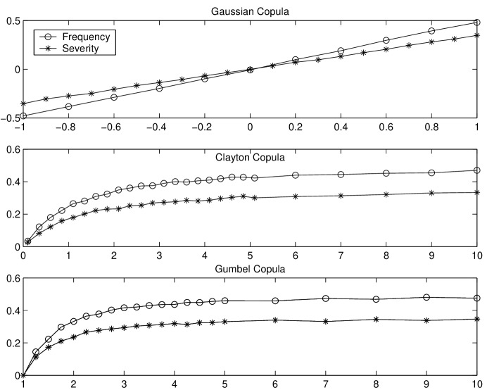
Figure 1: Spearman’s rank correlation, $\rho_{SR}\left(Z^{(1)},Z^{(2)}\right)$, between the annual losses vs copula parameter $\rho$, also see Section 3.  ($\circ$) $\rho_{SR}\left(Z^{(1)},Z^{(2)}\right)$ vs copula parameter $\rho$ between frequency risk profiles $\Lambda^{(1)}_{t}$ and $\Lambda^{(2)}_{t}$; ($\ast$) $\rho_{SR}\left(Z^{(1)},Z^{(2)}\right)$ vs copula parameter $\rho$ between severity risk profiles $\Psi_{t}^{(1)}$ and $\Psi_{t}^{(2)}$.

These parameters correspond to $\bm{\theta}_{\Lambda}$ and $\bm{\theta}_{\Psi}$ in Model Assumptions 2.1. In Figure 1, we present three cases where $C\left(\cdot|\rho\right)$ is a Gaussian, Clayton or Gumbel copula under both scenario 1 and scenario 2. In each of these examples we vary the parameter of the copula model $\rho$ from weak to strong dependence. The annual losses are not Gaussian distributed and to measure the dependence between the annual losses we use a non-linear rank correlation measure, Spearman’s rank correlation, denoted by $\rho_{SR}(Z_{t}^{(1)},Z_{t}^{(2)})$. The Spearman’s rank correlation between the annual losses was estimated using $10,000$ simulated years for each value of $\rho$. In these and other numerical experiments we conducted, the range of possible dependence between the annual losses of different risks induced by the dependence between risk profiles is very wide and should be flexible enough to model dependence in practice. Note, the degree of induced correlation can be further extended by working with more flexible copula models at the expense of estimation of a larger number of model parameters.

4 Bayesian Inference: combining different data sources

In this section we estimate the model introduced in Section 2 using a Bayesian inference method. To achieve this we must consider that the requirements of Basel II AMA (see BIS, p.152) clearly state that: ”Any operational risk measurement system must have certain key features to meet the supervisory soundness standard set out in this section. These elements must include the use of internal data, relevant external data, scenario analysis and factors reflecting the business environment and internal control systems”. Hence, Basel II requires that OpRisk models include use of several different sources of information. We will demonstrate that to satisfy such requirements it is important that methodology such as the one we develop in this paper be considered in practice to ensure one can soundly combine these different data sources.

It is widely recognized that estimation of OpRisk frequency and severity distributions cannot be done solely using historical data. The reason is the limited ability to predict future losses in a banking environment which is constantly changing. Assume that a new policy was introduced in a financial institution with the intention of reducing an OpRisk loss. This cannot be captured in a model based solely on historical loss data.

For the above reasons, it is very important to include Scenario Analysis (SA) in OpRisk modelling. SA is a process undertaken by banks to identify risks; analyze past events experienced internally and jointly with other financial institutions including near miss losses; consider current and planned controls in the banks, etc. Usually, it involves surveying of experts through workshops. A template questionnaire is developed to identify weaknesses, strengths and other factors. As a result an imprecise, value driven quantitative assessment of risk frequency and severity distributions is obtained. On its own, SA is very subjective and we argue it should be combined (supported) by actual loss data analysis. It is not unusual that correlations between risks are attempted to be specified by experts in the financial institution, typically via SA.

External loss data is also an important source of information which should be incorporated into modelling. There are several sources available to obtain external loss data, for a discussion on some of the data related issues associated with external data see Peters and Teruads (2007).

Additionally, the combination of expert opinions with internal and external data is a difficult problem and complicated ad-hoc procedures are used in practice. Some prominent risk professionals in industry have argued that statistically consistent combining of these different data sources is one of the most pertinent and challenging aspects of OpRisk modelling. It was quoted in Davis (2006) ”Another big challenge for us is how to mix the internal data with external data; this is something that is still a big problem because I don’t think anybody has a solution for that at the moment” and ”What can we do when we don’t have enough data [$\cdots$] How do I use a small amount of data when I can have external data with scenario generation? [$\cdots$] I think it is one of the big challenges for operational risk managers at the moment.”. Using the methodology that we develop in this paper, one may combine these data sources in a statistically sound approach, addressing these important practical questions that practitioners are facing under Basel II AMA.

Bayesian inference methodology is well suited to combine different data sources in OpRisk, for example see Shevchenko and Wüthrich (2006). A closely related credibility theory toy example was considered in Bühlmann, Shevchenko and Wüthrich (2007). We also note that in general questions of Bayesian model choice must be addressed, adding to this there is the additional complexity that estimation of the required posterior distributions will typically require MCMC, see Peters and Sisson (2006).

A Bayesian model to combine three data sources (internal data, external data and expert opinion) for the case of a single risk cell was presented in Lambrigger, Shevchenko and Wüthrich (2007). In this paper we extend this approach to the case of many risk cells with the dependence between risks introduced as in Section 2. Hereafter, for illustrative purposes we restrict to modelling frequencies only.

Hence, our objective will be to utilise Bayesian inference to estimate the parameters of the model through the combination of expert opinions and observed loss data (internal and external).

We note that as part of this Bayesian model formualtion an information flow can be incorporated into the model. This could be introduced in many forms. The most obvious example involves incorporation of new data from actual observed losses. However, we stress that more general ideas are possible. For example, if new information becomes available (new policy introduced, etc) then experts can update their prior distributions to incorporate this information into the model.

Additionally, under a Bayesian model we note that SA could naturally form part of a subjective Bayesian prior elicitation procedure, see O’Hagan (2006).

4.1 Modelling frequencies for a single risk cell

Here we follow the Lambrigger, Shevchenko and Wüthrich (2007) approach to combine different data sources for one risk cell in the case of the Model Assumptions 2.1.

Define a model in which every risk cell of a financial company $j\in\{1,\ldots,J\}$ is characterized by a risk characteristic $\Theta_{\Lambda}^{(j)}$ that describes the frequency risk profile $\Lambda_{t}^{(j)}$ in risk cell $j$. This $\Theta_{\Lambda}^{(j)}$ represents a vector of unknown distribution parameters of risk profile $\Lambda^{(j)}_{t}$. The true value of $\Theta_{\Lambda}^{(j)}$ is not known and modelled as a random variable. A priori, before having any company specific information, the prior distribution of $\Theta_{\Lambda}^{(j)}$ is based on external data only. Our aim then is to specify the distribution of $\Theta_{\Lambda}^{(j)}$ when we have company specific information about risk cell $j$ such as observed losses and expert opinions. This is achieved by developing a Bayesian model and numerical estimation of relevant quantities is performed via MCMC methods. For simplicity, in this section, we drop the risk cell specific superscript $j$ since we concentrate on modelling frequencies for single risk cell $j$, where $\Theta_{\Lambda}^{(j)}$ is a scalar $\Theta_{\Lambda}$ and all other parameters are assumed known.

Model Assumptions 4.1

Assume that risk cell $j$ has a fixed, deterministic volume $V$ (i.e. number of transactions, etc.).

1. The risk characteristics $\Theta_{\Lambda}$ of risk cell $j$ has prior distribution: $\Theta_{\Lambda}\sim\Gamma(a,b)$ for given parameters $a>0$ and $b>0$.

2. Given $\Theta_{\Lambda}=\theta_{\Lambda}$, $(\Lambda_{1},N_{1}),\ldots,(\Lambda_{T+1},N_{T+1})$ are i.i.d. and the intensity of events of year $t\in\{1,\ldots,T+1\}$ has conditional marginal distribution $\Lambda_{t}\sim\Gamma(\alpha,\alpha/\theta_{\Lambda})$ for a given parameter $\alpha>0$.

3. Given $\Theta=\theta_{\Lambda}$ and $\Lambda_{t}=\lambda_{t}$, the frequencies $N_{t}\sim Poi(V\lambda_{t})$.

4. The financial company has $K$ expert opinions $\Delta_{k}$, $k=1,\ldots,K$ about $\Theta_{\Lambda}$. Given $\Theta_{\Lambda}=\theta_{\Lambda}$, $\Delta_{k}$ and $(\Lambda_{t},N_{t})$ are independent for all $k$ and $t$, and $\Delta_{1},\ldots,\Delta_{K}$ are i.i.d. with $\Delta_{k}\sim\Gamma(\xi,\xi/\theta_{\Lambda})$.

Remarks 4.2

• In items 1) and 2) we choose a gamma distribution for the underlying parameters. Often, the available data is not sufficient to support such a choice. In such cases, in actuarial practice, one often chooses a gamma distribution. A gamma distribution is neither conservative nor aggressive and it has the advantage that it allows for transparent model interpretations. If other distributions are more appropriate then, of course, one should replace the gamma assumption. This can easily be done in our simulation methodology.

• Given that $\Theta_{\Lambda}\sim\Gamma(a,b)$, $E\left[\Theta_{\Lambda}\right]=a/b$ and $Var\left(\Theta_{\Lambda}\right)=a/b^{2}$. These are the prior two moments of the underlying risk characteristics $\Theta_{\Lambda}.$ The prior can be determined by external data (or regulator). In general, parameters $a$ and $b$ can be estimated by the maximum likelihood method using the data from all banks.

• Note that we have for the first moments

  $$E\left[\left.\Lambda_{t}\right|\Theta_{\Lambda}\right] = \Theta_{\Lambda},\text{ }E\left[\Lambda_{t}\right]=\frac{a}{b},\text{ }E\left[\left.N_{t}\right|\Theta_{\Lambda},\Lambda_{t}\right]=V~{}\Lambda_{t},$$

  $$E\left[\left.N_{t}\right|\Theta_{\Lambda}\right] = V~{}\Theta_{\Lambda},\text{ }E\left[N_{t}\right]=V~{}\frac{a}{b}.$$

  The second moments are given by

  $$Var\left(\left.\Lambda_{t}\right|\Theta_{\Lambda}\right) = \alpha^{-1}~{}\Theta_{\Lambda}^{2},~{}~{}\text{ }Var\left(\Lambda_{t}\right)=\alpha^{-1}~{}\frac{a^{2}}{b^{2}}+(\alpha^{-1}+1)~{}\frac{a}{b^{2}},$$

  $$Var\left(\left.N_{t}\right|\Theta_{\Lambda},\Lambda_{t}\right) = V~{}\Lambda_{t},\text{ }~{}~{}Var\left(\left.N_{t}\right|\Theta_{\Lambda}\right)=V~{}\Theta_{\Lambda}+V^{2}~{}\alpha^{-1}~{}\Theta_{\Lambda}^{2},$$ (4.1)

  $$Var\left(N_{t}\right) = V~{}\frac{a}{b}+V^{2}~{}\alpha^{-1}~{}\frac{a^{2}}{b^{2}}+V^{2}~{}(\alpha^{-1}+1)~{}\frac{a}{b^{2}}.$$

  For model interpretation purposes, consider the results for the coefficient of variation (CV), a convenient dimensionless measure of uncertainty commonly used in the insurance industry:

  $$\lim_{V\rightarrow\infty}CV^{2}\left(\left.N_{t}\right|\Theta_{\Lambda}\right)=\lim_{V\rightarrow\infty}\frac{Var\left(\left.N_{t}\right|\Theta_{\Lambda}\right)}{E^{2}\left[\left.N_{t}\right|\Theta_{\Lambda}\right]}=\alpha^{-1}>0,$$ (4.2)

  and

  $$\lim_{V\rightarrow\infty}CV^{2}\left(N_{t}\right)=\lim_{V\rightarrow\infty}\frac{Var\left(N_{t}\right)}{E^{2}\left[N_{t}\right]}=\alpha^{-1}+\left(\alpha^{-1}+1\right)~{}a^{-1}>0.$$ (4.3)

  That is, our model makes perfect sense from a practical perspective. Namely, as volume increases, $V\rightarrow\infty$, there always remains a non-diversifiable element, see (4.2) and (4.3). This is exactly what has been observed in practice and what regulators require from internal models. Note, if we model $\Lambda_{t}$ as constant and known then $\lim_{V\rightarrow\infty}CV^{2}\left(N_{t}|\Lambda_{t}\right)\rightarrow 0$.

• Contrary to the developments in Lambrigger, Shevchenko and Wüthrich (2007), where the intensity $\Lambda_{t}$ was constant overtime, now $\Lambda_{t}$ is a stochastic process. From a practical point of view, it is not plausible that the intensity of the annual counts is constant over time. In such a setting parameter risks completely vanish if we have infinitely many observed years or infinitely many expert opinions, respectively (see Theorem 3.6 (a) and (c) in Lambrigger, Shevchenko and Wüthrich (2007)). This is because $\ \Lambda_{t}$ can then be perfectly forecasted. In the present model, parameter risks will also decrease with increasing information. As we gain information the posterior standard deviation of $\Theta_{\Lambda}$ will converge to $0$. However, since $\Lambda_{T+1}$ viewed from time $T$ is always random, the posterior standard deviation for $\Lambda_{T+1}$ will be finite.

• Note that, conditionally given $\Theta_{\Lambda}=\theta_{\Lambda}$, $N_{t}$ has a negative binomial distribution with probability weights for $n\geq 0$,

  $$P\left.\left[N_{t}=n\right|\theta_{\Lambda}\right]={\binom{{\alpha+n-1}}{{n}}}\left(\frac{\alpha}{\alpha+\theta_{\Lambda}V}\right)^{\alpha}\left(\frac{\theta_{\Lambda}V}{\alpha+\theta_{\Lambda}V}\right)^{n}.$$ (4.4)

  That is, at this stage we could directly work with a negative binomial distribution. As we will see below, only in the marginal case can we work with (4.4). In the multidimensional model we require $\Lambda_{t}$.

• $\Delta_{k}$ denotes the expert opinion of expert $k$ which predicts the true risk characteristics $\Theta_{\Lambda}$ of his company. We have

  $$E\left.\left[\Delta_{k}\right|\Theta_{\Lambda}\right] = E\left.\left[\Lambda_{j}\right|\Theta_{\Lambda}\right]=E\left.\left[N_{j}/V\right|\Theta_{\Lambda}\right]=\Theta_{\Lambda},$$

  $$Var\left.\left(\Delta_{k}\right|\Theta_{\Lambda}\right) = \Theta_{\Lambda}^{2}/\xi,~{}~{}\text{ }CV\left.\left(\Delta_{k}\right|\Theta_{\Lambda}\right)=\xi^{-1/2}.$$ (4.5)

  That is, the relative uncertainty CV in the expert opinion does not depend on the value of $\Theta_{\Lambda}$. That means that $\xi$ can be given externally, e.g. by the regulator, who is able to give a lower bound to the uncertainty. Moreover, we see that the expert predicts the average frequency for his company. Alternatively, $\xi$ can be estimated using method of moments as presented in Lambrigger, Shevchenko and Wüthrich (2007).

Denote $\Lambda_{1:T}=\left(\Lambda_{1},\ldots,\Lambda_{T}\right)$, $N_{1:T}=\left(N_{1},\ldots,N_{T}\right)$ and $\Delta_{1:K}=\left(\Delta_{1},\ldots,\Delta_{K}\right)$. Then the joint posterior density of the random vector $(\Theta_{\Lambda},\Lambda_{1:T})$ given observations $N_{1}=n_{1},\ldots,N_{T}=n_{T}$, $\Delta_{1}=\delta_{1},\ldots,\Delta_{K}=\delta_{K}$ is by Bayes’ Theorem

$$\pi(\theta_{\Lambda},\lambda_{1:T}|n_{1:T},\delta_{1:K})\propto\pi\left(n_{1:T}|\theta_{\Lambda},\lambda_{1:T}\right)\pi\left(\lambda_{1:T}|\theta_{\Lambda}\right)\pi\left(\delta_{1:K}|\theta_{\Lambda}\right)\pi\left(\theta_{\Lambda}\right).$$ (4.6)

Here, the likelihood terms and the prior are made explicit,

$$\pi\left(n_{1:T}|\theta_{\Lambda},\lambda_{1:T}\right)\pi\left(\lambda_{1:T}|\theta_{\Lambda}\right) = \prod_{t=1}^{T}\frac{(V\lambda_{t})^{n_{t}}}{n_{t}!}\frac{(\alpha/\theta_{\Lambda})^{\alpha}}{\Gamma(\alpha)}\lambda_{t}^{\alpha-1}\exp\left\{-\lambda_{t}\left(V+\alpha/\theta_{\Lambda}\right)\right\},$$ (4.7)

$$\pi\left(\delta_{1:K}|\theta_{\Lambda}\right) = \prod_{k=1}^{K}\frac{(\xi/\theta_{\Lambda})^{\xi}}{\Gamma(\xi)}~{}\delta_{k}^{\xi-1}~{}\exp\left\{-\delta_{k}\xi/\theta_{\Lambda}\right\},$$ (4.8)

$$\pi\left(\theta_{\Lambda}\right) = \frac{b^{a}}{\Gamma(a)}~{}\theta_{\Lambda}^{a-1}~{}\exp\left\{-\theta_{\Lambda}b\right\}.$$ (4.9)

Note that the intensities $\Lambda_{1},\ldots,\Lambda_{T}$ are non-observable. Therefore we take the integral over their densities to obtain the posterior distribution of the random variable $\Theta_{\Lambda}$ given $\left(N_{1:T},\Delta_{1:K}\right)$

$$\pi\left(\theta_{\Lambda}|n_{1:T},\delta_{1:K}\right)\propto \prod_{t=1}^{T}{\binom{{\alpha+n_{t}-1}}{{n_{t}}}}\left(\frac{\alpha}{\alpha+\theta_{\Lambda}V}\right)^{\alpha}\left(\frac{\theta_{\Lambda}V}{\alpha+\theta_{\Lambda}V}\right)^{n_{t}}$$

$$\times\prod_{k=1}^{K}\frac{(\xi/\theta_{\Lambda})^{\xi}}{\Gamma(\xi)}~{}\delta_{k}^{\xi-1}~{}\exp\left\{-\delta_{k}\xi/\theta_{\Lambda}\right\}\frac{b^{a}}{\Gamma(a)}~{}\theta_{\Lambda}^{a-1}~{}\exp\left\{-\theta_{\Lambda}b\right\}$$

$$\ \ \propto \left(\frac{1}{\alpha+\theta_{\Lambda}V}\right)^{T\alpha+\sum_{t=1}^{T}n_{t}}~{}\theta_{\Lambda}^{a-K\xi+\sum_{t=1}^{T}n_{t}-1}~{}\exp\left\{-\theta_{\Lambda}b-\frac{\xi}{\theta_{\Lambda}}\sum_{k=1}^{K}\delta_{k}\right\}.$$ (4.10)

Given $\Theta_{\Lambda}$, the distribution of the number of losses $N_{t}$ is negative binomial. Hence, one could start with a negative binomial model for $N_{t}$. The reason for the introduction of the random intensities $\Lambda_{t}$ is that we will utilize them to model dependence between different risk cells, by introducing dependence between $\Lambda_{t}^{(1)},\ldots,\Lambda_{t}^{(J)}$.

Typically, a closed form expression for the marginal posterior function of $\Theta_{\Lambda}$, given $\left(N_{1:T},\Delta_{1:K}\right)$ can not be obtained, except in this single risk cell setting. In general, we will integrate out the latent variables $\Lambda_{1},\ldots,\Lambda_{T}$ numerically through a MCMC approach to obtain an empirical distribution for the posterior of $\pi\left(\theta_{\Lambda}|n_{1:T},\delta_{1:K}\right)$. This empirical posterior distribution then allows for the simulation of $\Lambda_{T+1}$ and $N_{T+1}$, respectively, conditional on the observations $\left(N_{1:T},\Delta_{1:K}\right)$.

4.2 Modelling frequencies for multiple risk cells

As in the previous section we will illustrate our methodology by presenting the frequency model construction. In this section we will extend the single risk cell frequency model to the general multiple risk cell setting. This will involve formulation of the multivariate posterior distribution.

Model Assumptions 4.3 (multiple risk cell frequency model)

Consider J risk cells. Assume that every risk cell $j$ has a fixed, deterministic volume $V^{(j)}$.

1. The risk characteristic $\bm{\Theta}_{\Lambda}=(\Theta_{\Lambda}^{(1)},\ldots,\Theta_{\Lambda}^{(J)})$ has a $J$-dimensional prior density $\pi(\bm{\theta}_{\Lambda})$. The copula parameters $\bm{\theta}_{\rho}$ are modelled by a random vector $\bm{\Theta}_{\rho}$ with the prior density $\pi\left(\bm{\theta}_{\rho}\right)$; $\bm{\Theta}_{\Lambda}$ and $\bm{\Theta}_{\rho}$ are independent.

2. Given $\bm{\Theta}_{\Lambda}=\bm{\theta}_{\Lambda}$ and $\bm{\Theta}_{\rho}=\bm{\theta}_{\rho}$: $(\bm{\Lambda}_{1},\bm{N}_{1}),\ldots,(\bm{\Lambda}_{T+1},\bm{N}_{T+1})$ are i.i.d. and the intensities $\bm{\Lambda}_{t}$ $=(\Lambda_{t}^{(1)},\ldots,\Lambda_{t}^{(J)})$ have a $J$ -dimensional conditional density with marginal distributions $\Lambda_{t}^{\left(j\right)}\sim G\left(\cdot|\theta_{\Lambda}^{\left(j\right)}\right)=\Gamma\left(\alpha^{\left(j\right)},\alpha^{\left(j\right)}/\theta_{\Lambda}^{\left(j\right)}\right)$ and the copula $c(\cdot|\bm{\theta}_{\rho})$. Thus the joint density of $\bm{\Lambda}_{t}$ is given by

   $$\pi(\bm{\lambda}_{t}|\bm{\theta}_{\Lambda},\bm{\theta}_{\rho})=c\left(G(\lambda_{t}^{(1)}|\theta_{\Lambda}^{(1)}),\ldots,G(\lambda_{t}^{(J)}|\theta_{\Lambda}^{(J)})|\bm{\theta}_{\rho}\right)\prod_{j=1}^{J}\pi(\lambda_{t}^{(j)}|\theta_{\Lambda}^{(j)}),$$ (4.11)

   where $\pi\left(\cdot|\theta_{\Lambda}^{\left(j\right)}\right)$ denotes the marginal density.

3. Given $\bm{\Theta}_{\Lambda}=\bm{\theta}_{\Lambda}$ and $\bm{\Lambda}_{t}=\bm{\lambda}_{t}$, the number of claims are independent with
   $N_{t}^{(j)}\sim Poi(V^{(j)}\lambda_{t}^{(j)}),j=1,\ldots,J$.

4. There are expert opinions $\bm{\Delta}_{k}=(\Delta_{k}^{(1)},\ldots,\Delta_{k}^{(J)})$, $k=1,\ldots,K$. Given $\bm{\Theta}_{\Lambda}=\bm{\theta}_{\Lambda}$: $\bm{\Delta}_{k}$ and $(\bm{\Lambda}_{t},\bm{N}_{t})$ are independent for all $k$ and $t$; and $\Delta_{k}^{(j)}$ are all independent with $\Delta_{k}^{(j)}\sim\Gamma(\xi^{(j)},\xi^{(j)}/\theta_{\Lambda}^{(j)})$.

For convenience of notation, define:

• $\bm{\Lambda}_{1:T}=\left[\left(\Lambda_{1}^{\left(1\right)},\ldots,\Lambda_{1}^{\left(J\right)}\right),\left(\Lambda_{2}^{\left(1\right)},\ldots,\Lambda_{2}^{\left(J\right)}\right),\ldots,\left(\Lambda_{T}^{\left(1\right)},\ldots,\Lambda_{T}^{\left(J\right)}\right)\right]$ - Frequency intensities for all risk profiles and years;

• $\bm{N}_{1:T}=\left[\left(N_{1}^{\left(1\right)},\ldots,N_{1}^{\left(J\right)}\right),\left(N_{2}^{\left(1\right)},\ldots,N_{2}^{\left(J\right)}\right),\ldots,\left(N_{T}^{\left(1\right)},\ldots,N_{T}^{\left(J\right)}\right)\right]$ - Annual number of losses for all risk profiles and years;

• $\bm{\Delta}_{1:K}=\left[\left(\Delta_{1}^{\left(1\right)},\ldots,\Delta_{1}^{\left(J\right)}\right),\left(\Delta_{2}^{\left(1\right)},\ldots,\Delta_{2}^{\left(J\right)}\right),\ldots,\left(\Delta_{K}^{\left(1\right)},\ldots,\Delta_{K}^{\left(J\right)}\right)\right]$ - Expert opinions on mean frequency intensities for all experts and risk profiles.

Prior Structure $\pi\left(\bm{\theta}_{\Lambda}\right)$ and $\pi\left(\bm{\theta}_{\rho}\right).$ In the following examples, a priori, the risk characteristics $\Theta_{\Lambda}^{(j)}$ are independent Gamma distributed: $\Theta_{\Lambda}^{(j)}\sim\Gamma(a^{(j)},b^{(j)})$ with hyper-parameters $a^{(j)}>0$ and $b^{(j)}>0$. This means that a priori the risk characteristics for the different risk classes are independent. That is, if the company has a bad risk profile in risk class $j$ then the risk profile in risk class $i$ need not necessarily also be bad. Dependence is then modelled through the dependence between the intensities $\Lambda^{(1)}_{t},\ldots,\Lambda^{(J)}_{t}$. If this is not appropriate then, of course, this can easily be changed by assuming dependence within $\bm{\Theta}_{\Lambda}.$

In the simulation experiments below we consider cases when the copula is parameterized by a scalar $\theta_{\rho}$. Additionally, we are interested in obtaining inferences on $\theta_{\rho}$ implied by the data only so we use an uninformative constant prior on the ranges [-1,1], (0,30] and [1,30] in the case of Gaussian, Clayton and Gumbel copulas respectively.

Posterior density. The marginal posterior density of random vector $\left(\bm{\Theta}_{\Lambda},\Theta_{\rho}\right)$ given data of counts $\bm{N}_{1}=\bm{n}_{1},\ldots,\bm{N}_{T}=\bm{n}_{T}$ and expert opinions $\bm{\Delta}_{1}=\bm{\delta}_{1},\ldots,\bm{\Delta}_{K}=\bm{\delta}_{K}$ is

$$\pi\left(\bm{\theta}_{\Lambda},\theta_{\rho}|\bm{n}_{1:T},\bm{\delta}_{1:K}\right)= \prod_{t=1}^{T}\int\pi\left(\bm{\theta}_{\Lambda},\theta_{\rho},\bm{\lambda}_{t}|\bm{n}_{1:T},\bm{\delta}_{1:K}\right)d\bm{\lambda}_{t}$$

$$\propto \prod_{t=1}^{T}\left(\int~{}\prod_{j=1}^{J}\exp\left\{-V^{(j)}\lambda_{t}^{(j)}\right\}~{}\frac{(V^{(j)}\lambda_{t}^{(j)})^{n_{t}^{(j)}}}{n_{t}^{(j)}!}~{}\pi(\bm{\lambda}_{t}|\bm{\theta}_{\Lambda},\theta_{\rho})~{}d\bm{\lambda}_{t}\right)$$

$$\times\prod_{k=1}^{K}\prod_{j=1}^{J}\left(\frac{(\xi^{(j)}/\theta_{\Lambda}^{(j)})^{\xi^{(j)}}}{\Gamma(\xi^{(j)})}~{}(\delta_{k}^{(j)})^{\xi^{(j)}-1}~{}\exp\left\{-\delta_{k}^{(j)}\xi^{(j)}/\theta_{\Lambda}^{(j)}\right\}\right)$$

$$\times\prod_{j=1}^{J}\frac{(b^{(j)})^{a^{(j)}}}{\Gamma(a^{(j)})}~{}(\theta_{\Lambda}^{(j)})^{a^{(j)}-1}~{}\exp\left\{-b^{(j)}\theta_{\Lambda}^{(j)}\right\}\pi\left(\theta_{\rho}\right).$$ (4.12)

5 Simulation Methodology - Slice sampler

Posterior (4.12) involves integration and sampling from this distribution is difficult. Here we present a specialized MCMC simulation methodology known as a Slice sampler to sample from the desired target posterior distribution $\pi(\bm{\theta}_{\Lambda},\theta_{\rho},\bm{\lambda}_{1:T}|\bm{n}_{1:T}$, $\bm{\delta}_{1:K})$. Marginally taken samples of $\bm{\Theta}_{\Lambda}$ and $\Theta_{\rho}$ are samples from $\pi\left(\bm{\theta}_{\Lambda},\theta_{\rho}|\bm{n}_{1:T},\bm{\delta}_{1:K}\right)$ which can be used to make inference for required quantities.

It will be convenient to define the exclusion operators, $\bm{\Lambda}_{1:T}^{(-i,-j)}$, $\bm{\Lambda}_{1:T\backslash k}$ and $\bm{\Theta}_{\Lambda}^{(-j)}$. For example:

• $\bm{\Lambda}_{1:T}^{\left(-2,-1\right)}=\left[\left(\Lambda_{1}^{\left(1\right)},\ldots,\Lambda_{1}^{\left(J\right)}\right),\left(\Lambda_{2}^{\left(2\right)},\ldots,\Lambda_{2}^{\left(J\right)}\right),\ldots,\left(\Lambda_{T}^{\left(1\right)},\ldots,\Lambda_{T}^{\left(J\right)}\right)\right]$ - Frequency intensities for all risk profiles and years, excluding risk profile 1 from year 2;

• $\bm{\Lambda}_{1:T\backslash 2}=\left[\left(\Lambda_{1}^{\left(1\right)},\ldots,\Lambda_{1}^{\left(J\right)}\right),\left(\Lambda_{3}^{\left(1\right)},\ldots,\Lambda_{3}^{\left(J\right)}\right),\ldots,\left(\Lambda_{T}^{\left(1\right)},\ldots,\Lambda_{T}^{\left(J\right)}\right)\right]$ - Frequency intensities for all risk profiles and years, excluding all profiles for year 2;

• $\bm{\Theta}_{\Lambda}^{(-j)}=\left[\Theta_{\Lambda}^{\left(1\right)},\ldots,\Theta_{\Lambda}^{\left(j-1\right)},\Theta_{\Lambda}^{\left(j+1\right)},\ldots,\Theta_{\Lambda}^{\left(J\right)}\right].$

Sampling from $\pi\left(\bm{\theta}_{\Lambda},\theta_{\rho},\bm{\lambda}_{1:T}|\bm{n}_{1:T},\bm{\delta}_{1:K}\right)$ or $\pi\left(\bm{\theta}_{\Lambda},\theta_{\rho}|\bm{n}_{1:T},\bm{\delta}_{1:K}\right)$ via closed form inversion sampling or via rejection sampling is not typically an option. There are many reasons for this. Firstly, only for specific copula models will closed form tractable expression for the marginal $\pi\left(\bm{\theta}_{\Lambda},\theta_{\rho}|\bm{n}_{1:T},\bm{\delta}_{1:K}\right)$ be attainable, certainly not for the models we consider in this paper. Secondly, even for the expression of the joint posterior $\pi\left(\bm{\theta}_{\Lambda},\theta_{\rho},\bm{\lambda}_{1:T}|\bm{n}_{1:T},\bm{\delta}_{1:K}\right)$ it is typically only possible to sample from the conditional distributions sequentially via numerical inversion sampling techniques which is highly computational and inefficient in high dimensions. Additionally, we would like a technique which is independent of the potentially arbitrary choice in specifying a copula function for the dependence between $\Lambda_{t}^{(1)},\ldots,\Lambda_{t}^{(J)}$. Hence, we utilize an MCMC framework which we make general enough to work for any choice of copula model, developed next.

5.1 Bayesian Parameter Estimation

We separate the analysis into two parts. Firstly, we condition on knowledge of the copula parameters $\theta_{\rho}=\rho$, where $\rho$ denotes the true copula parameters used to generate the data. This allows us to demonstrate that if the copula parameters $\theta_{\rho}$ are known, we can perform estimation of other parameters accurately under joint inference. The second part involves joint estimation of $\theta_{\rho}$ and $\bm{\theta}_{\Lambda}$ to demonstrate the accuracy of the joint inference procedure developed. Note that, the model for this second part has not been formally introduced but is a simple extension of Model Assumptions 4.3.

5.1.1 Conditional on a priori knowledge of copula parameter

Here we assume the copula parameter has been estimated a priori and so estimation only involves model parameters. Such a setting may arise for example if the copula parameter is already estimated via a ML estimator. The proposed sampling procedure we develop is a particular class of algorithms in the toolbox of MCMC methods. It is an alternative to a Gibbs sampler known as a univariate Slice sampler. We note that to implement a Gibbs sampler or a univariate Slice sampler one needs to know the form of the full conditional distributions. However, unlike the basic Gibbs sampler the Slice sampler does not require sampling from these full conditional distributions. Derivations of the posterior full conditionals,

$$\pi(\theta_{\Lambda}^{(j)}|\bm{\theta}_{\Lambda}^{(-j)},\bm{\lambda}_{1:T},\bm{n}_{1:T},\bm{\delta}_{1:K},\theta_{\rho}) \propto \pi(\bm{\lambda}_{1:T}|\bm{\theta}_{\Lambda}^{(-j)},\theta_{\Lambda}^{(j)},\theta_{\rho})\pi(\bm{\delta}_{1:K}|\bm{\theta}_{\Lambda}^{(-j)},\theta_{\Lambda}^{(j)})$$ (5.1)

$$\times\pi(\bm{\theta}_{\Lambda}^{(-j)}|\theta_{\Lambda}^{(j)})\pi(\theta_{\Lambda}^{(j)}),$$

$$\pi(\lambda_{t}^{(j)}|\bm{\theta}_{\Lambda},\bm{\lambda}_{1:T}^{(-t,-j)},\bm{n}_{1:T},\bm{\delta}_{1:K},\theta_{\rho}) \propto \pi(\bm{n}_{1:T}|\bm{\lambda}_{1:T}^{(-t,-j)},\lambda_{t}^{(j)})\pi(\bm{\lambda}_{t}^{(-j)},\lambda_{t}^{(j)}|\bm{\theta}_{\Lambda},\theta_{\rho})$$ (5.2)

are presented in Appendix B.

5.1.2 Joint Inference of marginal and copula parameters

To include the estimation of the copula parameter $\theta_{\rho}$ jointly with the parameters $\bm{\Theta}_{\Lambda}$ and latent intensities $\bm{\Lambda}_{1:T}$ in our Bayesian framework, we assume that it is constant in time and model it by a random variable $\Theta_{\rho}$ with some prior density $\pi(\theta_{\rho})$. The full conditional posterior of the copula parameter, denoted $\pi\left(\theta_{\rho}|\bm{\theta}_{\Lambda},\bm{\lambda}_{1:T},\bm{n}_{1:T},\bm{\delta}_{1:K}\right),$ is given by

$$\pi\left(\theta_{\rho}|\bm{\theta}_{\Lambda},\bm{\lambda}_{1:T},\bm{n}_{1:T},\bm{\delta}_{1:K}\right)\propto\pi(\bm{\lambda}_{1:T}|\bm{\theta}_{\Lambda},\theta_{\rho})\pi\left(\theta_{\rho}\right),$$ (5.3)

For the full derivation of the scalar case see, Appendix B.

In the following section we provide intuition for our choice of univariate Slice sampler as compared to alternative Markov chain algorithms. In particular we describe the advantages that the Slice sampler has compared to more standard Markov chain samplers, though we also point out the additional complexity involved. We verify the validity of the Slice sampling algorithm for those not familiar with this specialized algorithm and we then describe some intricacies associated with implementation of the algorithm. This is followed by a discussion of some extensions we developed when analyzing the OpRisk model. The technical details of the actual algorithm are provided in Appendix C.

5.2 Slice sampling

The full conditionals given in equations (5.1), (5.2), (5.3) do not take standard explicit closed forms and typically the normalizing constants are not known in closed form. Therefore this will exclude straightforward inversion or basic rejection sampling being used to sample from these distributions. Therefore one may adopt a Metropolis Hastings (MH) within Gibbs sampler to obtain samples, see for example Gilks, Richardson and Spiegelhalter (1996) and Robert and Casella (2004) for detailed expositions of such approaches. To utilize such algorithms it is important to select a suitable proposal distribution. Quite often in high dimensional problems such as ours, this requires tuning of the proposal for a given target distribution. Hence, one incurs a significant additional computational expense in tuning the proposal distribution parameters off-line so that mixing of the resulting Markov chain is sufficient. An alternative not discussed here would include an Adaptive Metropolis Hastings within Gibbs sampling algorithm, see Atachade and Rosenthal (2005) and Rosenthal (2009). Here we take a different approach which utilizes the full conditional distributions, known as a univariate Slice sampler, see Neal (2003). We demonstrate how effective a univariate Slice sampler is for our model.

Slice sampling was developed with the intention of providing a ”black box” approach for sampling from a target distribution which may not have a simple form. The Slice sampling methodology we develop will be automatically tailored to the desired target posterior. As such it does not require pretuning and in many cases will be more efficient than a MH within Gibbs sampler. The reason for this, pointed out by Neal (2003), is that a MH within Gibbs has two potential problems. The first arises when a MH approach attempts moves which are not well adapted to local properties of the density, resulting in slow mixing of the Markov chain. Secondly, the small moves arising from the slow mixing typically lead to traversal of a region of posterior support in the form of a Random Walk. Therefore, $L^{2}$ steps are required to traverse a distance that could be traversed in only $L$ steps if moving consistently in the same direction. A univariate Slice sampler can adaptively change the scale of the moves proposed avoiding problems that can arise with the MH sampler when the appropriate scale of proposed moves varies over the support of the distribution.

A single iteration of the Slice sampling distribution for a toy example is presented in Figure 2. The intuition behind Slice sampling arises from the fact that sampling from a univariate distribution $p\left(\theta\right)$ can always be achieved by sampling uniformly from the region under the distribution $p\left(\theta\right).$ Obtaining a Slice sample follows two steps: sample a value $u_{l}\sim U\left[0,p\left(\theta_{l-1}\right)\right]$ and then sample a value uniformly from $A_{l},$ $\theta_{l}\sim U\left[A_{l}\right].$ This procedure is repeated and by discarding the auxiliary variable sample $u_{l}$ one obtains correlated samples $\theta_{l}^{\prime}s$ from $p\left(\theta_{l-1}\right)$. Neal (2003), demonstrates that a Markov chain $\left(U,\Theta\right)$ constructed in this way will have stationary distribution defined by a uniform distribution under $p\left(\theta\right)$ and the marginal of $\Theta$ has desired stationary distribution $p\left(\theta\right).$ Additionally, Mira and Tierney (2002) proved that the Slice sampler algorithm, assuming a bounded target distribution $p\left(\theta\right)$ with bounded support, is uniformly ergodic.

Similar to a deterministic scan Gibbs sampler, the simplest way to extend the Slice sampler to a multivariate distribution is by considering each full conditional distribution in turn. Note, discussion relating to the benefits provided by Random Walk behaviour suppression, as achieved by the Slice sampler, are presented in the context of non-reversible Markov chains, see Diaconis, Holmes and Neal (2000).

Additionally, we only need to know the target full conditional posterior up to normalization, see Neal (2003) p. 710. This is important in this example since solving the normalizing constant in this model is not possible analytically. To make more precise the intuitive description of the Slice sampler presented above, we briefly detail the argument made by Neal on this point. Suppose we wish to sample from a distribution for a random vector $\mathbf{\Theta}\in\mathbb{R}^{n}$ whose density $p\left(\bm{\theta}\right)$ is proportional to some function $f\left(\bm{\theta}\right)$. This can be achieved by sampling uniformly from the $\left(n+1\right)$-dimensional region that lies under the plot of $f\left(\bm{\theta}\right)$. This is formalised by introducing the auxiliary random variable $U$ and defining a joint distribution over $\bm{\Theta}$ and $U$ which is uniform over the region $\left\{\left(\bm{\Theta,}U\right):0<u<f\left(\bm{\theta}\right)\right\}$ below the surface defined by $f\left(\bm{\theta}\right)$, given by

$$p\left(\bm{\theta,}u\right)=\left\{\begin{array}[]{cc}{1/Z,}&\text{if }0<u<f\left(\bm{\theta}\right),\\ {0,}&\text{ otherwise,}\end{array}\right.$$

where $Z=\int f\left(\bm{\theta}\right)d\bm{\theta}$ . Then the target marginal density for $\mathbf{\Theta}$ is given by

$$p\left(\bm{\theta}\right)=\int_{0}^{f\left(\bm{\theta}\right)}\frac{1}{Z}du=\frac{f\left(\bm{\theta}\right)}{Z},$$

as required. There are many possible procedures to obtain samples of $\left(\mathbf{\Theta,}U\right)$. The details of the implemented algorithm undertaken in this paper are provided in Appendix C.

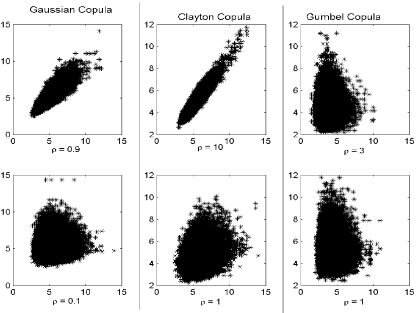
Figure 3: Scatter plot of $\left(\Theta_{\Lambda}^{(1)},\Theta_{\Lambda}^{(2)}\right)$ from $\pi\left(\bm{\theta}_{\Lambda}|\bm{n}_{1:20},\bm{\delta}_{1:1},\lambda_{1:20},\theta_{\rho}\right)$ with Gaussian, Clayton and Gumbel copulas $C(\cdot|\theta_{\rho}=\rho)$ between frequency risk profiles. Top row: strong correlation. Bottom row: weak correlation

Extensions
We note that in the Bayesian model we develop, in some cases strong correlation between the parameters of the model will be present in the posterior, see Figure 3. In more extreme cases, this can cause slow rates of convergence of a univariate sampler to reach the ergodic regime, translating into longer Markov Chain simulations. In such a situation several approaches can be tried to overcome this problem. The first involves the use of a mixture transition kernel combining local and global moves. For example, we suggest local moves via a univariate Slice sampler and global moves via an Independent Metropolis Hastings (IMH) sampler with adaptive learning of its covariance structure, such an approach is known as a hybrid sampler, see comparisons in Brewer, Aitken and Talbot (1996). Alternatively, for the global move if determination of level sets in multiple dimensions is not problematic, for the model under consideration, then some of the multivariate Slice sampler approaches designed to account for correlation between parameters can be incorporated, see Neal (2003) for details. This is beyond the scope of this paper.

Another approach to break correlation between parameters in the posterior is via transformation of the parameter space. If the transformation is effective this will reduce correlation between parameters of the transformed target posterior. Sampling can then proceed in the transformed space, and then samples can be transformed back to the original space. It is not always straightforward to find such transformations.

A third alternative is based on Simulated Tempering, introduced by Marinari and Parisi (1992) and discussed extensively in Geyer and Thompson (1995). In particular a special version of Simulated Tempering, first introduced by Neal (1996) can be utilised in which on considers a sequence of target distributions $\left\{\pi_{l}\right\}$ constructed such that they correspond to the objective posterior in the following way,

$$\pi_{l}=\left[\pi\left(\bm{\theta}_{\Lambda},\bm{\lambda}_{1:T},\theta_{\rho}\bm{|n}_{1:T},\bm{\delta}_{1:K}\right)\right]^{\gamma_{l}}$$

with sequence $\left\{\gamma_{l}\right\}.$ Then one uses the Slice sampling algorithm presented and replaces $\pi$ with $\pi_{l}$.

Running a Markov chain such that at each iteration $l$ we target posterior $\pi_{l}$ and then only keeping samples from the Markov chain corresponding to situations in which $\gamma_{l}=1$ can result in a significant improvement in exploration around the posterior support. This can overcome slow mixing arising from a univariate sampling regime. The intuition for this is that for values of $\gamma_{l}<<1$ the target posterior is almost uniform over the space, resulting in large moves being possible around the support of the posterior, then as $\gamma_{l}$ returns to a value of $1$, several iterations later, it will be in potentially new unexplored regions of posterior support.

As an extension we developed a Simulated Tempering Slice sampler to obtain samples from the posterior $p\left(\bm{\theta}_{\Lambda},\bm{\lambda}_{1:T},\theta_{\rho}\bm{|n}_{1:T},\bm{\delta}_{1:K}\right)$. In our development we utilize a sine function, $\gamma_{l}=\text{min}\left(\text{sin}\left(\frac{2\pi}{1000}l\right)+1,1\right)$, for $\gamma_{l}$ which has its amplitude truncated to ensure it ranges between $\left(0,1\right]$. That is the function is truncated at $\gamma_{l}=1$ for extended iteration periods for our simulation index $l$ to ensure the sampler spends significant time sampling from the actual posterior distribution.

We note that application of the Tempering proved useful and improved mixing of the Markov chain. However, for simulation examples presented in the remainder of this paper it was sufficient to use the basic univariate Slice sampler presented previously, which is more computationally efficient than the Tempered version.

Note, in the application of Tempering one must discard many simulated states of the Markov chain, whenever $\gamma_{l}\neq 1$. There is however a computational way to avoid discarding these samples, see Gramacy, Samworth and King (2007).

Finally, we note that there are several alternatives to a MH within Gibbs sampler such as a basic Gibbs sampler combined with Adaptive Rejection sampling (ARS), Gilks and Wild (1992). Note ARS requires distributions to be log concave. Alternatively an adaptive version of this known as the Adaptive Metropolis Rejection sampler could be used, see Gilks, Best and Tan (1995).

6 Results

In this section we demonstrate and compare the performance of our sampling methodology on several different copula models. We intend to demonstrate the appropriate behaviour of our Bayesian models as a function of the number of annual years, in the presence of highly biased expert opinions. This will be achieved through simulation studies using the sampling techniques detailed above to perform inference on model parameters. The intention will be to demonstrate the appropriate convergence and accuracy as a function of data sample size. Hereafter, we study the case of dependence between intensities of two risks and set risk cell volumes $V^{\left(1\right)}=V^{\left(2\right)}=1.$

6.1 Estimation of model if copula parameter is known

Here, we study the estimation of model parameters in two cases. The first case involves two low frequency risks. In the second case, one risk has low frequency while another risk has high frequency. In these two cases we present results for the univariate Slice sampler under scenarios involving: data generated independently for each risk profile and data generated using a Gaussian, Clayton and Gumbel copulas.

Only one expert opinion is assumed for each risk. We present the parameter estimates as a function of data size for each of the specified correlation levels. That is, we study the accuracy of the parameter estimates as the number of observations increases. Simulation results are obtained by creating independently 20 data sets each of length 20 years, then for each data set simulations are performed for subsets of the data going for 1, 2, 5, 10, 15 and 20 years. We then average the performance of posterior estimates over these independent simulations. The Markov chains are run for 50,000 iterations with 10,000 iterations discarded as burnin. The simulation time depends on the number of risk profiles, the number of observations and expert opinions and the length of the Markov chain. In performing the analysis we studied three cases and in each case we performed the following steps,

1. Simulate a data set of appropriate number of years according to the procedure specified in Appendix A.

2. Obtain correlated MCMC samples from the target posterior distribution after discarding burnin samples, $\left\{\bm{\theta}_{\Lambda,l},\bm{\lambda}_{1:T,l}\right\},l=1001,\ldots,50000$.

3. Estimate desired posterior quantities such as posterior mean of parameters of interest and posterior standard deviations.

4. Repeat stages 1 - 3 for 20 independent data realisations and then average the results.

• Joint: The results are obtained by MCMC samples taken from $\pi\left(\bm{\theta}_{\Lambda},\bm{\lambda}_{1:T}|\bm{n}_{1:T},\bm{\delta}_{1:K},\theta_{\rho}\right)$ with the correct copula model and copula parameter used in the sampler. This is the procedure that should be performed in a real application.

• Marginal: Results are obtained by MCMC samples taken from

  $$\pi\left(\bm{\theta}_{\Lambda},\bm{\lambda}_{1:T}|\bm{n}_{1:T},\bm{\delta}_{1:K},\theta_{\rho}\right) = \prod\limits_{j=1}^{J}\pi\left({\theta_{\Lambda}}^{\left(j\right)},{\lambda}_{1:T}^{\left(j\right)}|\bm{n}_{1:T},\bm{\delta}_{1:K},\theta_{\rho}\right)$$

  $$= \prod\limits_{j=1}^{J}\pi\left({\theta_{\Lambda}}^{\left(j\right)}|\bm{n}_{1:T},\bm{\delta}_{1:K},\theta_{\rho}\right)$$

  which is the posterior in the case of independence. This is equivalent to marginal estimation where single risk cell data is analyzed separately, see Section 4.1.

• Benchmark: To verify the results we also consider the case where we assume perfect knowledge of the realized random process for random vector $\bm{\Lambda}_{1:T}$. We then perform inference on $\bm{\Theta}_{\Lambda}$ without the additional uncertainty arising from estimating $\bm{\Lambda}_{1:T}.$ In this regard this represents a benchmark for which we may compare the performance of our simulations. In particular, it is obtained by samples taken from $\pi\left(\bm{\theta}_{\Lambda}|\bm{\lambda}_{1:T},\bm{n}_{1:T},\bm{\delta}_{1:K},\theta_{\rho}\right)$ conditional on the true simulated realizations of random variables $\bm{\Lambda}_{1:T}$.

Example 1: low frequency risk profiles. We set the true parameter values of $\Theta_{\Lambda}^{(1)}$ and $\Theta_{\Lambda}^{(2)}$ to be $\theta_{true}^{\left(1\right)}=5$ and $\theta_{true}^{\left(2\right)}=5$ respectively. Also we choose the expert’s opinion on the true parameters to be an underestimate in risk profile 1 with $\Delta_{1}^{\left(1\right)}=2$ and an overestimate for risk profile 2 with $\Delta_{1}^{\left(2\right)}=8.$ The model parameters were set to $\xi^{\left(1\right)}=\xi^{\left(2\right)}=2$, $\alpha^{\left(1\right)}=\alpha^{\left(2\right)}=2$, and prior distribution parameters $a^{(1)}=a^{(2)}=2$, $b^{(1)}=b^{(2)}=2.5$. The results for this simulation study, presented in Tables 1 and 2, show the appropriate convergence of the estimates of parameters $\Theta_{\Lambda}^{(1)}$ and $\Theta_{\Lambda}^{(2)}$ as a function of the data size, demonstrating how well this simulation procedure works under these models. In addition we note that as expected from credibility theory we observe that joint estimation is better than the marginal, i.e. the posterior standard deviations for $\Theta_{\Lambda}^{(1)}$ and $\Theta_{\Lambda}^{(2)}$ are less when joint estimation is used. In addition the rate of convergence of the posterior mean for $\Theta_{\Lambda}$ to the true value is faster under the joint estimation. Note, the standard errors in the posterior mean and standard deviation were calculated and found to be strictly in the range of 1-5% for the simulations presented.

In Figure 3, corresponding to Gaussian, Clayton and Gumbel copula models respectively, we demonstrate the estimated density $\pi\left(\bm{\theta}_{\Lambda}|\bm{\lambda}_{1:T},\bm{n}_{1:T},\bm{\delta}_{1:K},\theta_{\rho}\right)$ if we had perfect knowledge of the latent process parameters $\bm{\Lambda}_{1:T}$. In this way we compare the exact posterior with perfect knowledge of the correlation structure as captured by the copula model which here we assume is known. Obtaining these plots involved a particular realized data set of length 20 years. For all copulas two values of $\theta_{\rho}$ were considered: $\theta_{\rho}=0.9$ and $\theta_{\rho}=0.1$ for Gaussian copula; $\theta_{\rho}=10$ and $\theta_{\rho}=1$ for Clayton copula; and $\theta_{\rho}=3$ and $\theta_{\rho}=1.1$ for the Gumbel copula. These plots of the joint marginal posterior distribution of $\bm{\Theta}_{\Lambda}$ demonstrate clearly that the standard practice in the industry of performing marginal estimation of risk profiles will lead to incorrect results when estimating quantities based on the distribution of $\bm{\Theta}_{\Lambda}$.

Example 2: one low frequency and one high frequency risk profile. We set the true values of $\Theta_{\Lambda}^{(1)}$ and $\Theta_{\Lambda}^{(2)}$ to be $\theta_{true}^{\left(1\right)}=5$ and $\theta_{true}^{\left(2\right)}=10$ respectively. Also we choose the expert’s opinion on the true parameters to be an under estimate in risk profile 1 with $\Delta_{1}^{\left(1\right)}=2$ and an over estimate for risk profile 2 with $\Delta_{1}^{\left(2\right)}=13.$ The model parameters were set to $\xi^{\left(1\right)}=\xi^{\left(2\right)}=2$, $\alpha^{\left(1\right)}=2,\alpha^{\left(2\right)}=2$, $a^{(1)}=a^{(2)}=2$, $b^{(1)}=2.5,b^{(2)}=5$. The simulation results and comparisons are developed in the same approach as Example 1 and again the standard errors in the estimates were in the range 1-5%. The results can be found in Tables 3 and 4.

6.2 Joint estimation of marginal and copula parameters

Here we estimate $\Theta_{\Lambda}^{(1)},\Theta_{\Lambda}^{(2)}$ and $\Theta_{\rho}$ jointly. For this example, the model settings from Example 1 were used and one data set of length 20 years randomly generated was utilized. The simulation was performed by taking 150,000 iterations of the sampler and discarding the first 20,000 as burnin. Results for these simulations are contained in Table 5.

These results demonstrate that our model and estimation methodology is successfully able to estimate jointly the risk profiles and the correlation parameter. This is seen to be the case for all the models we consider in this paper. It is also clear that with few observations, e.g. $T\leq 5$, and a vague prior for the copula parameter, it will be difficult to accurately estimate the copula parameter. This is largely due to the fact that the posterior distribution in this case is diffuse. Additionally, with a small amount of data it appears that accurately estimating the copula parameter is most difficult in the Gumbel model. However, as the number of observations increases the accuracy of the estimate improves in all models and the estimates are reasonable in the case of $15$ or $20$ years of data. Additionally, we could further improve the accuracy of this prediction if we incorporated expert opinions into the prior specification of the copula parameter, instead of using a vague prior.

Overall, we have demonstrated that combination of all the relevant sources of data can be achieved under our model. Then with this study we show that our sampling methodology has the ability to estimate jointly all the model parameters including the copula parameter. This is a key step forward in model development and estimation for OpRisk models. We further envisage that one can extend this methodology to more sophisticated and flexible copula based models with more than one parameter. This should be relatively trivial since the methodology we developed applies directly. However, the challenge in the case of a more sophisticated copula model relates to finding a relevant choice of prior distribution on the correlation structure.

Full predictive distribution. As a final comment in this section we point out an important additional outcome of obtaining samples from the joint posterior distribution of the model parameters and the correlation. This relates to construction of the full predictive annual loss distribution, accounting for parameter uncertainty.

Typically practitioners will take point estimates of all parameters and then condition on these point estimates to empirically construct the predictive distribution and then calculate risk measures to be reported such as VaR. Here we comment that a more robust approach to prediction can now be performed. Using our methodology, we can construct the full predictive distribution after removing the parameter uncertainty from the model considered, including the uncertainty arising from the correlation parameter. To achieve this we would consider the full predictive distribution:

$$\pi\left(Z_{T+1}|n_{1:T},\delta_{1:T}\right)=\int\pi\left(Z_{T+1}|\bm{\theta}_{\Lambda},\theta_{\rho}\right)\pi\left(\bm{\theta}_{\Lambda},\theta_{\rho}|n_{1:T},\delta_{1:T}\right)d\bm{\theta}_{\Lambda}d\theta_{\rho}.$$ (6.1)

Here, we used the model assumptions that given $\bm{\Theta}_{\Lambda}$ and $\Theta_{\rho}$ we have that $Z_{T+1}$ is independent from the observations $(N_{1:T},\Delta_{1:K})$. In practice to obtain samples from this full predictive distribution involves taking the steps demonstrated in Appendix A with a minor modification. If one wanted to simulate $L$ annual losses from the full predictive distribution, this would involve first running the Slice sampler for $L$ iterations after burnin. Then for each iteration $l$ one would use the state of the Markov chain $\left(\bm{\theta}_{\Lambda,l},\theta_{\rho,l}\right)$ in the simulation procedure detailed in Appendix A. We also note that it is trivial under our methodology to extend this full predictive distribution sampling to the case of frequency and severities.

7 Discussion

This paper introduced a dynamic OpRisk model which allows for significant flexibility in correlation structures introduced between risk profiles. Next a Bayesian framework was established to allow inference and estimation under this model to be performed, whilst at the same time allowing incorporation of alternative data sources into the inferential procedure. Then a novel simulation procedure was developed for the Bayesian model presented, in the case of dependence between frequency risk profiles. Simulations were performed to demonstrate the accuracy of this procedure in multiple bivariate examples. Comparisons were made between marginal estimation and a benchmark estimation procedure. In all simulations, the estimation of the model parameters was accurate and behaviour of the estimates of posterior mean and standard deviation presented, smoothed over multiple data realizations, was as expected. Initially the influence of the biased expert opinion observation influenced the results and as the size of the data set for actual annual loss counts grew, the estimations improved in accuracy. Clearly, the joint estimation will outperform marginal estimation when forming predictions of future counts and rates in year $T+1$, given estimates based on data up to year $T$. Additionally, we demonstrated highly accurate estimation of the copula parameter, jointly with the model parameters.

Additionally, simulations were performed in the models $J=5$ and $J=10$ for the Clayton copula model in which the copula parameter is also unknown. Though the simulation time was increased as a factor of the number of risk cells, the results and performance were as presented for the bivariate models, making this approach suitable for practical purposes.

Finally, the main objective of the paper is to preset the framework for the multivariate problem and to demonstrate estimation in this setting. Application of the framework to real data is the subject of further research. In this paper, the estimation procedure is presented for frequencies only but it can be extended in the same manner as presented to severities.

Appendix A Appendix: Simulation of annual losses

In general, given marginal and copula parameters $\left(\bm{\theta}_{\Lambda},\bm{\theta}_{\Psi},\bm{\theta}_{\rho}\right)$, the simulation of the annual losses for year $t=T+1$, when risk profiles are dependent, can be done as described below.

1. Simulate $2J$-variate $u_{1},\ldots,u_{J},v_{1},\ldots,v_{J}$ from a $2J$ dimensional copula $C(\cdot|\bm{\theta}_{\rho}).$

2. Calculate ${\lambda}_{t}^{\left(j\right)}=G^{-1}\left(u_{j}|\theta_{\Lambda}^{(j)}\right)$ and $\psi_{t}^{\left(j\right)}=H^{-1}\left(v_{j}|\theta_{\Psi}^{(j)}\right),j=1,\ldots,J$

3. Sample $n_{t}^{(j)}$ from $P\left(\cdot|\lambda_{t}^{(j)}\right),j=1,\ldots,J$.

4. Sample iid $x_{s}^{(j)}(t),s=1,\ldots,n_{t}^{(j)},j=1,\ldots,J$ from $F\left(\cdot|{\psi}_{t}^{(j)}\right)$.

5. Calculate annual losses $z_{t}^{\left(j\right)}=\sum\limits_{s=1}^{n_{t}^{\left(j\right)}}x_{s}^{(j)}\left(t\right),j=1,\ldots,J$.

6. Repeat Steps 1-5, $K$ times to get $K$ random samples of the annual losses $z_{t}^{\left(j\right)}$.

Note, to simulate from the full predictive distribution of annual losses, add simulation of $\left(\bm{\theta}_{\Lambda},\bm{\theta}_{\Psi},\bm{\theta}_{\rho}\right)$ from the posterior distribution (e.g. using Slice sampler methodology) as an extra step before Step 1. Simulation of the random variates from a copula in Step 1 in the case of Gaussian, Clayton and Gumbel copulas can be done as described below.

Gaussian copula:

1. Simulate $d$-variate $x_{1},\ldots,x_{d}$ from $\Phi_{N}\left(\bm{0,}\Sigma\right)$, where $\Phi_{N}\left(\bm{0,}\Sigma\right)$ is a Normal distribution with zero means, unit variances and correlation matrix $\Sigma$.

2. Calculate $u_{1}=F_{N}(x_{1}),\ldots,u_{d}=F_{N}(x_{d})$. Obtained $(u_{1},\ldots,u_{d})$ is a $d$-variate from a Gaussian copula.

Archimedean copulas: The Clayton and Gumbel copulas are members of the Archimedean family of copulas. The $d$-dimensional Archimedean copulas can be written as

$$C\left(u_{1},\ldots,u_{d}|\rho\right)=\phi^{-1}\left(\phi\left(u_{1}\right)+\cdots+\phi\left(u_{d}\right)\right)$$ (A.1)

with $\phi$ a decreasing function known as the generator for the given copula, see Frees and Valdez (1998). The generator and inverse generator for the Clayton ($\phi_{C}$) and Gumbel ($\phi_{G}$) copulas are given by

$$\phi_{C}\left(t\right) = \left(t^{-\rho}-1\right);\hskip 14.22636pt\phi_{C}^{-1}\left(s\right)=\left(1+s\right)^{-\frac{1}{\rho}};$$

$$\phi_{G}\left(t\right) = \left(-\ln t\right)^{\rho};\hskip 14.22636pt\phi_{G}^{-1}\left(s\right)=\exp\left(-s^{\frac{1}{{}^{\rho}}}\right),$$ (A.2)

where $\rho$ is a copula parameter. Simulation from such a copula can be achieved following the algorithm provided in Melchiori (2006):

1. Sample $d$ independent random variates $v_{1},\ldots,v_{d}$ from a uniform distribution $U[0,1]$.

2. Simulate $y$ from $D(\cdot)$ such that Laplace transform of $D$ satisfies $\mathcal{L}\left(D\right)=\phi^{-1}$ and $D\left(0\right)=0.$

3. Find $s_{i}=-\left(\ln v_{i}\right)/y$ for $i=1,\ldots,d$

4. Calculate $u_{i}=\phi^{-1}\left(s_{i}\right)$ for $i=1,\ldots,d.$

The obtained $(u_{1},\ldots,u_{d})$ is a $d$-variate from $d$-dimensional Archimedean copula. What remains is to define the relevant distribution $D(\cdot)$ for the Clayton and Gumbel Copulas. For the Clayton copula, $D(\cdot)$ is a Gamma distribution with shape parameter given by $\rho^{-1}$ and unit scale. For the Gumbel copula, $D(\cdot)$ is from the $\alpha-$stable family $S_{\alpha}\left(\beta,\gamma,\delta\right)$ with the following parameters shape $\alpha=\rho^{-1}$, skewness $\beta=1$, scale $\gamma=(\cos(\frac{1}{2}\pi/\rho))^{\rho}$ and location $\delta=0.$ In the Gumbel case, the density for $D$ has no analytic form and the simulation from this distribution can be achieved using the algorithm from Nolan (2007) to efficiently generate the required samples from the univariate stable distribution.

Appendix B Appendix: Full conditional posterior distributions

Note, in Part 1 and Part 2 we are conditioning on the copula parameter $\theta_{\rho}$, this notation is dropped for simplicity. It is only explicitly introduced in Part 3.

Part 1: Using Bayes’ theorem

$$\pi \left(\theta_{\Lambda}^{\left(j\right)}|\bm{\theta}_{\Lambda}^{\left(-j\right)},\bm{\lambda}_{1:T},\bm{n}_{1:T},\bm{\delta}_{1:K}\right)\propto\pi\left(\bm{\theta}_{\Lambda}^{\left(-j\right)},\bm{\lambda}_{1:T},\bm{n}_{1:T},\bm{\delta}_{1:K}|\theta_{\Lambda}^{\left(j\right)}\right)\pi\left(\theta_{\Lambda}^{\left(j\right)}\right)$$

$$=\pi\left(\bm{\lambda}_{1:T},\bm{n}_{1:T},\bm{\delta}_{1:K}|\bm{\theta}_{\Lambda}^{\left(-j\right)},\theta_{\Lambda}^{\left(j\right)}\right)\pi\left(\bm{\theta}_{\Lambda}^{\left(-j\right)}|\theta_{\Lambda}^{\left(j\right)}\right)\pi\left(\theta_{\Lambda}^{\left(j\right)}\right).$$ (B.1)

Using the model structure to exploit conditional independence properties we note that

$$\pi \left(\bm{\lambda}_{1:T},\bm{n}_{1:T},\bm{\delta}_{1:K}|\bm{\theta}_{\Lambda}^{\left(-j\right)},\theta_{\Lambda}^{\left(j\right)}\right)=\pi\left(\bm{n}_{1:T},\bm{\lambda}_{1:T}|\bm{\theta}_{\Lambda}^{\left(-j\right)},\theta_{\Lambda}^{\left(j\right)}\right)\pi\left(\bm{\delta}_{1:K}|\bm{\theta}_{\Lambda}^{\left(-j\right)},\theta_{\Lambda}^{\left(j\right)}\right)$$

$$=\pi\left(\bm{n}_{1:T}|\bm{\lambda}_{1:T}\right)\pi\left(\bm{\lambda}_{1:T}|\bm{\theta}_{\Lambda}^{\left(-j\right)},\theta_{\Lambda}^{\left(j\right)}\right)\pi\left(\bm{\delta}_{1:K}|\bm{\theta}_{\Lambda}^{\left(-j\right)},\theta_{\Lambda}^{\left(j\right)}\right)$$ (B.2)

which specifies the full conditional distributions for the $j^{th}$ component $\Theta_{\Lambda}^{\left(j\right)}$ as

$$\pi \left(\theta_{\Lambda}^{\left(j\right)}|\bm{\theta}_{\Lambda}^{\left(-j\right)},\bm{\lambda}_{1:T},\bm{n}_{1:T},\bm{\delta}_{1:K}\right)\propto\pi\left(\bm{n}_{1:T}|\bm{\lambda}_{1:T}\right)$$

$$\hskip 28.45274pt\times\pi\left(\bm{\lambda}_{1:T}|\bm{\theta}_{\Lambda}^{\left(-j\right)},\theta_{\Lambda}^{\left(j\right)}\right)\pi\left(\bm{\delta}_{1:K}|\bm{\theta}_{\Lambda}^{\left(-j\right)},\theta_{\Lambda}^{\left(j\right)}\right)\pi\left(\bm{\theta}_{\Lambda}^{\left(-j\right)}|\theta_{\Lambda}^{\left(j\right)}\right)\pi\left(\theta_{\Lambda}^{\left(j\right)}\right)$$

$$\propto\pi\left(\bm{\lambda}_{1:T}|\bm{\theta}_{\Lambda}^{\left(-j\right)},\theta_{\Lambda}^{\left(j\right)}\right)\pi\left(\bm{\delta}_{1:K}|\bm{\theta}_{\Lambda}^{\left(-j\right)},\theta_{\Lambda}^{\left(j\right)}\right)\pi\left(\bm{\theta}_{\Lambda}^{\left(-j\right)}|\theta_{\Lambda}^{\left(j\right)}\right)\pi\left(\theta_{\Lambda}^{\left(j\right)}\right).$$ (B.3)

Part 2: The next full conditional distribution we must specify is given by

$$\pi \left(\lambda_{t}^{\left(j\right)}|\bm{\theta}_{\Lambda},\bm{\lambda}_{1:T}^{\left(-t,-j\right)},\bm{n}_{1:T},\bm{\delta}_{1:K}\right)\propto\pi\left(\bm{\theta}_{\Lambda},\bm{\lambda}_{1:T}^{\left(-t,-j\right)},\bm{n}_{1:T},\bm{\delta}_{1:K}|\lambda_{t}^{\left(j\right)}\right)\pi\left(\lambda_{t}^{\left(j\right)}\right)$$

$$=\pi\left(\bm{\lambda}_{1:T}^{\left(-t,-j\right)},\bm{n}_{1:T},\bm{\delta}_{1:K}|\bm{\theta}_{\Lambda},\lambda_{t}^{\left(j\right)}\right)\pi\left(\bm{\theta}_{\Lambda}|\lambda_{t}^{\left(j\right)}\right)\pi\left(\lambda_{t}^{\left(j\right)}\right).$$ (B.4)

We then use conditional independence properties of the model to get

$$\pi \left(\bm{\lambda}_{1:T}^{\left(-t,-j\right)},\bm{n}_{1:T},\bm{\delta}_{1:K}|\bm{\theta}_{\Lambda},\lambda_{t}^{\left(j\right)}\right)$$

$$=\pi\left(\bm{n}_{1:T}|\bm{\lambda}_{1:T}^{\left(-t,-j\right)},\lambda_{t}^{\left(j\right)}\right)\pi\left(\bm{\lambda}_{1:T}^{\left(-t,-j\right)}|\bm{\theta}_{\Lambda},\lambda_{t}^{\left(j\right)}\right)\pi\left(\bm{\delta}_{1:K}|\bm{\theta}_{\Lambda}\right)$$ (B.5)

giving the full conditional we are interested in, up to proportionality,

$$\pi \left(\lambda_{t}^{\left(j\right)}|\bm{\theta}_{\Lambda},\bm{\lambda}_{1:T}^{\left(-t,-j\right)},\bm{n}_{1:T},\bm{\delta}_{1:K}\right)\propto\pi\left(\bm{n}_{1:T}|\bm{\lambda}_{1:T}^{\left(-t,-j\right)},\lambda_{t}^{\left(j\right)}\right)$$

$$\times\pi\left(\bm{\delta}_{1:K}|\bm{\theta}_{\Lambda}\right)\pi\left(\bm{\lambda}_{1:T}^{\left(-t,-j\right)}|\bm{\theta}_{\Lambda},\lambda_{t}^{\left(j\right)}\right)\pi\left(\bm{\theta}_{\Lambda}|\lambda_{t}^{\left(j\right)}\right)\pi\left(\lambda_{t}^{\left(j\right)}\right).$$ (B.6)

We now demonstrate that this expression simplifies significantly. We can show that the terms $\pi\left(\bm{\lambda}_{1:T}^{\left(-t,-j\right)}|\bm{\theta}_{\Lambda},\lambda_{t}^{\left(j\right)}\right)\pi\left(\bm{\theta}_{\Lambda}|\lambda_{t}^{\left(j\right)}\right)\pi\left(\lambda_{t}^{\left(j\right)}\right)$ simplify as follows:

$$\pi \left(\bm{\lambda}_{1:T}^{\left(-t,-j\right)}|\bm{\theta}_{\Lambda},\lambda_{t}^{\left(j\right)}\right)\pi\left(\bm{\theta}_{\Lambda}|\lambda_{t}^{\left(j\right)}\right)\pi\left(\lambda_{t}^{\left(j\right)}\right)=\frac{\pi\left(\bm{\theta}_{\Lambda},\bm{\lambda}_{1:T}^{\left(-t,-j\right)},\lambda_{t}^{\left(j\right)}\right)}{\pi\left(\bm{\theta}_{\Lambda},\lambda_{t}^{\left(j\right)}\right)}\pi\left(\bm{\theta}_{\Lambda}|\lambda_{t}^{\left(j\right)}\right)\pi\left(\lambda_{t}^{\left(j\right)}\right)$$

$$=\frac{\pi\left(\bm{\lambda}_{1:T}^{\left(-t,-j\right)},\lambda_{t}^{\left(j\right)}|\bm{\theta}_{\Lambda}\right)\pi\left(\bm{\theta}_{\Lambda}\right)}{\pi\left(\bm{\theta}_{\Lambda}|\lambda_{t}^{\left(j\right)}\right)\pi\left(\lambda_{t}^{\left(j\right)}\right)}\pi\left(\bm{\theta}_{\Lambda}|\lambda_{t}^{\left(j\right)}\right)\pi\left(\lambda_{t}^{\left(j\right)}\right)$$

$$=\pi\left(\bm{\lambda}_{1:T}^{\left(-t,-j\right)},\lambda_{t}^{\left(j\right)}|\bm{\theta}_{\Lambda}\right)\pi\left(\bm{\theta}_{\Lambda}\right).$$ (B.7)

Finally, we are left with the full conditional distribution

$$\pi \left(\lambda_{t}^{\left(j\right)}|\bm{\theta}_{\Lambda},\bm{\lambda}_{1:T}^{\left(-t,-j\right)},\bm{n}_{1:T},\bm{\delta}_{1:K}\right)\propto\pi\left(\bm{n}_{1:T}|\bm{\lambda}_{1:T}^{\left(-t,-j\right)},\lambda_{t}^{\left(j\right)}\right)$$

$$\hskip 28.45274pt\times\pi\left(\bm{\delta}_{1:K}|\bm{\theta}_{\Lambda}\right)\pi\left(\bm{\lambda}_{1:T}^{\left(-t,-j\right)}|\bm{\theta}_{\Lambda},\lambda_{t}^{\left(j\right)}\right)\pi\left(\bm{\theta}_{\Lambda}|\lambda_{t}^{\left(j\right)}\right)\pi\left(\lambda_{t}^{\left(j\right)}\right)$$

$$\propto\pi\left(\bm{n}_{1:T}|\bm{\lambda}_{1:T}^{\left(-t,-j\right)},\lambda_{t}^{\left(j\right)}\right)\pi\left(\bm{\lambda}_{1:T}^{\left(-t,-j\right)},\lambda_{t}^{\left(j\right)}|\bm{\theta}_{\Lambda}\right)$$

$$\propto\pi\left(\bm{n}_{1:T}|\bm{\lambda}_{1:T}^{\left(-t,-j\right)},\lambda_{t}^{\left(j\right)}\right)\pi\left(\bm{\lambda}_{t}^{\left(-j\right)},\lambda_{t}^{\left(j\right)}|\bm{\theta}_{\Lambda}\right).$$ (B.8)

Part 3: The full conditional distribution for the copula parameter is given by

$$\pi \left(\theta_{\rho}|\bm{\theta}_{\Lambda},\bm{\lambda}_{1:T},\bm{n}_{1:T},\bm{\delta}_{1:K}\right)\propto\pi\left(\bm{\theta}_{\Lambda},\bm{\lambda}_{1:T},\bm{n}_{1:T},\bm{\delta}_{1:K}|\theta_{\rho}\right)\pi\left(\theta_{\rho}\right)$$

$$\propto\pi\left(\bm{n}_{1:T}|\bm{\lambda}_{1:T}\right)\pi\left(\bm{\delta}_{1:K}|\bm{\theta}_{\Lambda}\right)\pi(\bm{\lambda}_{1:T}|\bm{\theta}_{\Lambda},\theta_{\rho})\pi\left(\bm{\theta}_{\Lambda}\right)\pi\left(\theta_{\rho}\right)$$

$$\propto\pi(\bm{\lambda}_{1:T}|\bm{\theta}_{\Lambda},\theta_{\rho})\pi\left(\theta_{\rho}\right).$$ (B.9)

Appendix C Appendix: Slice sampler algorithm.

Here, we provide the explicit details involved into implementation of a Slice sampler algorithm within a Gibbs sampler framework discussed in Section 5. The iterations of the Slice sampler are denoted by simulation index $l\in\mathbb{N}$.

Slice sampling:

1. Initialize $l=0$ the parameter vector $\left[\bm{\theta}_{\Lambda,0},\bm{\lambda}_{1:T,0},\theta_{\rho,0}\right]$ randomly or deterministically.

2. Repeat while $l\leq L$

   1. Set $\left[\bm{\theta}_{\Lambda,l},\bm{\lambda}_{1:T,l},\theta_{\rho,l}\right]=\left[\bm{\theta}_{\Lambda,l-1},\bm{\lambda}_{1:T,l-1},\theta_{\rho,l-1}\right]$

   2. Sample $j$ uniformly from set $\left\{1,2,\ldots,J\right\}$

      Sample new parameter value $\widetilde{\theta}_{\Lambda}^{\left(j\right)}$ from the full conditional posterior distribution $\pi\left(\theta_{\Lambda}^{\left(j\right)}|\bm{\theta}_{\Lambda,l}^{\left(-j\right)}\bm{,\lambda}_{1:T,l},\bm{n}_{1:T},\bm{\delta}_{1:K},\theta_{\rho,l}\right)$.

      Set $\theta_{\Lambda,l}^{\left(j\right)}=\widetilde{\theta}_{\Lambda}^{\left(j\right)}$.

   3. Sample $j$ uniformly from set $\left\{1,2,\ldots,J\right\}$ and $t$ uniformly from set $\left\{1,\ldots,T\right\}$

      Sample new parameter value $\widetilde{\lambda}_{t}^{\left(j\right)}$ from the full conditional posterior distribution $\pi\left(\lambda_{t}^{\left(j\right)}|\bm{\theta}_{\Lambda,l}\bm{,\lambda}_{1:T,l}^{\left(-t,-j\right)},\bm{n}_{1:T},\bm{\delta}_{1:K},\theta_{\rho,l}\right)$.

      Set $\lambda_{t,l}^{\left(j\right)}=\widetilde{\lambda}_{t}^{\left(j\right)}$.

   4. Sample new parameter value $\widetilde{\theta}_{\rho}$ from the full conditional posterior distribution

      $\pi\left(\theta_{\rho}|\bm{\theta}_{\Lambda,l}\bm{,\lambda}_{1:T,l},\bm{n}_{1:T},\bm{\delta}_{1:K}\right)$.

      Set $\theta_{\rho,l}=\widetilde{\theta}_{\rho}$.

3. $l=l+1$ and return to 2.

The sampling from the full conditional posteriors in stage 2 uses a univariate Slice sampler, see Figure 2. We present the case where we wish to sample the next iteration of the Markov chain from $\pi\left(\theta_{\Lambda}^{\left(j\right)}|\bm{\theta}_{\Lambda,l}^{\left(-j\right)},\bm{\lambda}_{1:T,l},\bm{n}_{1:T},\bm{\delta}_{1:K},\theta_{\rho}\right).$

Obtaining a sample using a univariate Slice sampler:

1.  Sample $u$ from a uniform distribution

$$U\left[0,\pi\left(\theta_{\Lambda,l}^{\left(j\right)}|\bm{\theta}_{\Lambda,l}^{\left(-j\right)}\bm{,\lambda}_{1:T,l},\bm{n}_{1:T},\bm{\delta}_{1:K},\theta_{\rho}\right)\right].$$

2.  Sample $\widetilde{\theta}_{\Lambda}^{\left(j\right)}$ uniformly from the intervals (level set)

$$A=\left\{\theta_{\Lambda}^{\left(j\right)}:\pi\left(\theta_{\Lambda}^{\left(j\right)}|\bm{\theta}_{\Lambda,l}^{\left(-j\right)}\bm{,\lambda}_{1:T,l},\bm{n}_{1:T},\bm{\delta}_{1:K},\theta_{\rho}\right)>u\right\}.$$

There are many approaches that could be used in determination of the level sets $A$ of our density

$$\pi\left(\theta_{\Lambda}^{\left(j\right)}|\bm{\theta}_{\Lambda,l}^{\left(-j\right)},\bm{\lambda}_{1:T,l},\bm{n}_{1:T},\bm{\delta}_{1:K},\theta_{\rho}\right),$$

see Neal (2003) [p.712, Section 4]. For simplicity in our proceeding examples we assume that we can restrict our parameter space to the finite ranges and we argue that this is reasonable since we can consider the finite bounds for example set according to machine precision for the smallest and largest number we can represent on our computing platform. This is not strictly required, but simplifies the coding of the algorithm. We then perform what Neal (2003) terms a stepping out and a shrinkage procedure, the details of which are contained in Neal (2003) [p.713, Figure 1]. The basic idea is that given a sampled vertical level $u$ then the level sets $A$ can be found by positioning an interval of width $w$ randomly around $\theta_{\Lambda,l}^{\left(j\right)}$. This interval is expanded in step sizes of width $w$ until both ends are outside the slice. Then a new state is obtained by sampling uniformly from the interval until a point in the slice $A$ is obtained. Points that fail can be used to shrink the interval.

Year	1	2	5	10	15	20
Independent
Marginal	3.72 (2.04)	4.10 (1.98)	4.08 (1.62)	4.64 (1.42)	5.13 (1.31)	5.24 (1.27)
Gaussian copula with ($\rho=0.9$)
Benchmark	4.32 (1.88)	4.50 (1.67)	4.84 (1.46)	5.17 (1.26)	5.19 (1.12)	5.21 (1.02)
Joint	3.91 (2.01)	4.41 (1.72)	4.37 (1.56)	4.76 (1.33)	5.10 (1.21)	4.95 (1.05)
Marginal	3.72 (2.05)	4.09 (1.97)	4.06 (1.61)	4.48 (1.37)	5.07 (1.29)	5.04 (1.13)
Clayton copula with ($\rho=10$)
Benchmark	4.81 (1.82)	5.17 (1.72)	5.13 (1.42)	4.96 (1.13)	5.10 (0.98)	5.00 (0.84)
Joint	4.19 (2.03)	4.92 (1.87)	5.05 (1.56)	4.87 (1.26)	4.96 (1.08)	4.90 (0.93)
Marginal	3.91 (2.12)	4.43 (2.10)	4.54 (1.74)	4.47 (1.36)	4.75 (1.22)	4.72 (1.08)
Gumbel copula with ($\rho=3$)
Benchmark	4.32 (1.98)	4.46 (1.70)	4.86 (1.41)	5.08 (1.16)	5.16 (1.01)	5.11 (0.88)
Joint	4.33 (2.06)	4.21 (1.80)	4.54 (1.56)	4.96 (1.23)	5.01 (1.05)	4.98 (0.93)
Marginal	3.84 (2.08)	3.76 (1.87)	4.17 (1.62)	4.63 (1.41)	4.74 (1.22)	4.72 (1.07)

Table 1: Average estimates of posterior mean and standard deviation of $\Theta_{\Lambda}^{\left(1\right)}$ for 20 data sets. Data are generated using different copula models as specified. The true values are $\theta_{true}^{\left(1\right)}=\theta_{true}^{\left(2\right)}=5.$

Year	1	2	5	10	15	20
Independent
Marginal	6.74 (2.74)	6.84 (2.59)	6.46 (2.16)	5.91 (1.67)	5.74 (1.40)	5.47 (1.31)
Gaussian ($\rho=0.9$)
Benchmark	5.98 (2.29)	5.84 (2.04)	5.46 (1.60)	5.47 (1.31)	5.43 (1.14)	5.41 (1.04)
Joint	6.37 (2.55)	6.01 (2.23)	5.63 (1.80)	5.40 (1.43)	5.43 (1.25)	5.36 (1.12)
Marginal	6.59 (2.72)	6.49 (2.54)	6.01 (2.07)	5.75 (1.64)	5.62 (1.43)	5.57 (1.26)
Clayton ($\rho=10$)
Benchmark	5.57 (1.91)	5.41 (1.69)	5.20 (1.40)	4.90 (1.10)	5.09 (0.96)	5.07 (0.85)
Joint	6.39 (2.48)	5.92 (1.92)	5.36 (1.64)	5.06 (1.22)	5.13 (1.17)	5.00 (1.02)
Marginal	6.69 (2.74)	6.56 (2.55)	5.92 (2.04)	5.40 (1.56)	5.37 (1.36)	5.24 (1.17)
Gumbel ($\rho=3$)
Benchmark	5.83 (2.35)	5.51 (2.02)	5.38 (1.57)	5.15 (1.18)	5.20 (1.02)	5.12 (0.89)
Joint	6.05 (2.47)	5.96 (2.17)	5.47 (1.76)	5.21 (1.27)	5.12 (1.07)	5.12 (0.94)
Marginal	6.42 (2.67)	6.26 (2.50)	5.92 (2.04)	5.67 (1.62)	5.52 (1.37)	5.36 (1.18)

Table 2: Average estimates of posterior mean and standard deviation of $\Theta_{\Lambda}^{\left(2\right)}$ for 20 data sets. The data are generated using different copula models as specified. The true values are $\theta_{true}^{\left(1\right)}=\theta_{true}^{\left(2\right)}=5$.

Year	1	2	5	10	15	20
Independent
Marginal	3.72 (2.04)	4.07 (1.97)	4.05 (1.61)	4.48 (1.37)	4.94 (1.26)	5.13 (1.13)
Gaussian ($\rho=0.9$)
Benchmark	4.07 (1.76)	4.22 (1.53)	4.61 (1.36)	5.10 (1.20)	5.10 (1.08)	5.20 (0.99)
Joint	3.86 (1.96)	4.39 (1.86)	4.46 (1.51)	4.84 (1.33)	5.10 (1.22)	5.24 (1.10)
Marginal	3.72 (2.04)	4.08 (1.97)	4.05 (1.61)	4.48 (1.37)	4.94 (1.26)	5.13 (1.13)
Clayton ($\rho=10$)
Benchmark	4.45 (1.65)	4.86 (1.55)	4.89 (1.32)	4.82 (1.07)	5.00 (0.95)	4.92 (0.83)
Joint	4.15 (2.01)	4.84 (1.95)	4.92 (1.59)	4.69 (1.33)	4.97 (1.20)	4.96 (1.04)
Marginal	3.98 (2.10)	4.53 (2.09)	4.54 (1.74)	4.47 (1.36)	4.74 (1.21)	4.72 (1.08)
Gumbel ($\rho=3$)
Benchmark	4.14 (1.90)	4.20 (1.58)	4.65 (1.32)	4.95 (1.11)	5.06 (0.97)	5.04 (0.87)
Joint	4.36 (2.16)	4.17 (1.85)	4.68 (1.57)	5.10 (1.34)	5.21 (1.21)	5.24 (1.01)
Marginal	3.84 (2.17)	3.75 (1.87)	4.17 (1.62)	4.64 (1.41)	4.75 (1.22)	4.79 (1.09)

Table 3: Average estimates of posterior mean and standard deviation of $\Theta_{\Lambda}^{\left(1\right)}$ for 20 data sets. Data are generated using different copula models as specified. The true values are $\theta_{true}^{\left(1\right)}=5$ and $\theta_{true}^{\left(2\right)}=10$.

Year	1	2	5	10	15	20
Independent
Marginal	10.89 (3.74)	10.78 (3.60)	10.18 (3.19)	9.70 (2.67)	9.64 (2.31)	9.48 (2.14)
Gaussian ($\rho=0.9$)
Benchmark	10.44 (3.48)	10.50 (3.24)	10.25 (2.81)	10.51 (2.39)	10.78 (2.05)	10.04 (1.88)
Joint	10.68 (3.63)	10.13 (3.35)	9.57 (2.87)	9.60 (2.36)	9.31 (2.03)	9.23 (1.82)
Marginal	10.89 (3.74)	10.78 (3.60)	10.18 (3.19)	9.70 (2.67)	9.64 (2.31)	9.48 (2.15)
Clayton ($\rho=10$)
Benchmark	10.04 (3.21)	10.07 (2.99)	9.88 (2.58)	9.59 (2.08)	9.97 (1.87)	9.97 (1.66)
Joint	10.58 (3.54)	10.03 (3.19)	9.29 (2.69)	9.82 (2.22)	9.93 (1.97)	9.78 (1.73)
Marginal	10.94 (3.75)	10.92 (3.61)	10.13 (3.17)	9.32 (2.60)	9.30 (2.25)	9.45 (1.96)
Gumbel ($\rho=3$)
Benchmark	10.10 (3.55)	9.88 (3.23)	10.08 (2.74)	9.98 (2.22)	10.17 (1.95)	10.06 (1.74)
Joint	10.10 (3.61)	10.18 (3.39)	9.44 (2.87)	9.98 (2.33)	9.85 (1.99)	9.63 (1.75)
Marginal	10.61 (3.76)	10.51 (3.59)	10.11 (3.17)	9.70 (2.66)	9.45 (2.27)	9.39 (1.98)

Table 4: Average estimates of posterior mean and standard deviation of $\Theta_{\Lambda}^{\left(2\right)}$ for 20 data sets. Data are generated using different copula models as specified. The true values are $\theta_{true}^{\left(1\right)}=5$ and $\theta_{true}^{\left(2\right)}=10$.

Year	1	2	5	10	15	20
Posterior mean and standard deviation for $\Theta_{\Lambda}^{(1)}$
Independent	2.81 (1.75)	4.71 (2.21)	3.05 (1.29)	4.90 (1.48)	4.38 (1.14)	5.13 (1.15)
Gaussian ($\rho=0.9$)	2.83 (1.74)	4.49 (2.02)	3.31 (1.38)	4.88 (1.29)	4.36 (1.10)	5.07 (1.09)
Clayton ($\rho=10$)	4.27 (2.04)	3.80 (1.76)	4.14 (1.46)	5.62 (1.45)	4.53 (1.04)	4.90 (0.99)
Gumbel ($\rho=3$)	2.81 (1.40)	2.59 (1.26)	3.08 (1.17)	4.28 (1.26)	4.51 (1.12)	4.91 (0.95)
Posterior mean and standard deviation for $\Theta_{\Lambda}^{(1)}$
Independent	10.24 (3.97)	9.56 (3.56)	9.48 (3.17)	9.10 (2.58)	9.33 (2.24)	9.55 (1.98)
Gaussian ($\rho=0.9$)	10.23 (3.92)	10.85 (3.52)	8.72 (2.95)	8.91 (2.12)	8.58 (2.04)	9.94 (1.85)
Clayton ($\rho=10$)	11.40 (3.58)	10.76 (3.47)	10.85 (3.10)	11.39 (2.60)	10.76 (2.27)	10.17 (2.03)
Gumbel ($\rho=3$)	12.27 (3.63)	11.26 (3.59)	9.11 (2.93)	9.54 (2.26)	9.91 (1.72)	9.88 (1.17)
Posterior mean and standard deviation for $\Theta_{\rho}$
Independent	0.20 (0.53)	0.10 (0.44)	-0.10 (0.38)	-0.02 (0.30)	-0.17 (0.28)	-0.12 (0.16)
Gaussian ($\rho=0.9$)	0.21 (0.54)	0.47 (0.39)	0.61 (0.30)	0.66 (0.24)	0.70 (0.19)	0.74 (0.15)
Clayton ($\rho=10$)	5.37 (2.81)	5.83 (2.66)	6.20 (2.52)	6.48 (2.25)	6.70 (2.11)	8.24 (1.88)
Gumbel ($\rho=3$)	16.41 (8.33)	16.59 (8.19)	16.39 (8.09)	9.42 (8.76)	5.12 (6.21)	3.90 (4.80)

Table 5: Posterior estimates for $\Theta_{\Lambda}^{\left(1\right)},\Theta_{\Lambda}^{\left(2\right)}$ and copula parameter $\Theta_{\rho}$. In this case a single data set is generated using different copula models as specified. Posterior standard deviations are given in brackets next to estimate. Joint estimation was used.

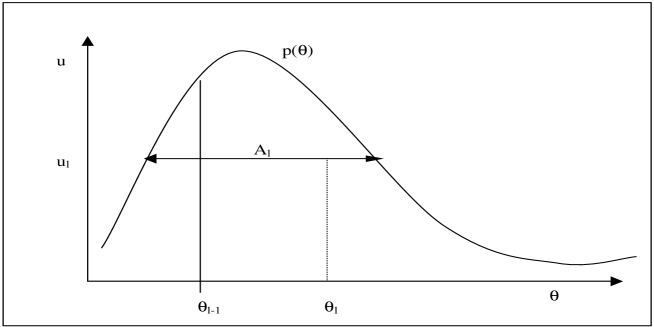
Figure 2: Markov chain created for $\Theta_{\Lambda}$ and auxiliary random variable $U$,
$\left(u_{1},\theta_{\Lambda,1}\right),\ldots,\left(u_{l-1},\theta_{\Lambda,l-1}\right),\left(u_{l},\theta_{\Lambda,l}\right),\ldots$ has stationary distribution with the desired marginal distribution $p\left(\theta_{\Lambda}\right).$

References

- [1] Artzner P., Delbaen F., Eber J.M. and Heath D. (1999). Coherent measures of risk. Mathematical Finance 9(3), 203-228.
- [2] Atchade Y. and Rosenthal, J. (2005). On adaptive Markov chain Monte Carlo algorithms. Bernoulli 11(5), 815-828.
- [3] Aue F. and Klakbrener, M. (2006). LDA at work: Deutsche Bank’s approach to quantifying operational risk. The Journal of Operational Risk 1(4), 49-95.
- [4] Bee M. (2005). Copula-based multivariate models with applications to risk management and insurance. Preprint, University of Trento, Available at www.gloriamundi.org.
- [5] BIS (June, 2006). International Convergence of Capital Measurement and Capital Standards. Basel Committee on Banking Supervision, Bank for International Settlements, Basel. www.bis.org.
- [6] Böcker K. and Klüppelberg C. (2008). Modelling and measuring multivariate operational risk with Levy copulas. The Journal of Operational Risk 3(2), 3-27.
- [7] Brewer M.J., Aitken C.G.G. and Talbot M. (1996). A comparison of hybrid strategies for Gibbs sampling in mixed graphical models. Computational Statistics and Data Analysis 21(3), 343-365.
- [8] Bühlmann H., Shevchenko P.V. and Wüthrich M.V. (2007). A ”Toy” model for operational risk quantification using Credibility theory. The Journal of Operational Risk 2(1), 3-19.
- [9] Chavez-Demoulin V., Embrechts P. and Nešlehová J. (2006). Quantitative models for Operational Risk: Extremes, dependence and aggregation. Journal of Banking and Finance 30(10), 2635-2658.
- [10] Cruz M. (ed.) (2004). Operational Risk Modelling and Analysis: Theory and Practice. Risk Books, London.
-
[11]
Davis E. (2006). Theory vs reality. OpRisk and Compliance
www.opriskandcompliance.com/public/showPage.html?page=345305. - [12] Diaconis P., Holmes S. and Neal R. M. (2000). Analysis of a non-reversible Markov chain sampler. Annals of Applied Probability 10, 726-752.
- [13] Embrechts P. and Frei M. (2009). Panjer recursion versus FFT for compound distributions. Mathematical Methods of Operations Research 69(3), 497-508.
- [14] Embrechts P., Lambrigger D.D. and Wüthrich M. (2009). Multivariate extremes and the aggregation of dependent risks: examples and counter-examples. Extremes 12(2), 107-127.
- [15] Embrechts P., Nešlehová J. and Wüthrich M. (2009). Additivity properties for Value-at-Risk under Archimedean dependence and heavy-tailedness. Insurance: Mathematics and Economics 44, 164-169.
- [16] Embrechts P. and Puccetti G. (2008). Aggregation operational risk across matrix structured loss data. The Journal of Operational Risk. 3(2), 29-44.
- [17] Frachot A., Moudoulaud O. and Roncalli T. (2004). Loss distribution approach in practice. The Basel Handbook: A Guide for Financial Practitioners. Ong M. (ed), Risk Books.
- [18] Frachot A., Roncalli T. and Salomon E. (2004). The correlation problem in operational risk. Group de Recherche Opérationnelle, France. Working paper, www.gloriamundi.org.
- [19] Frees E.W. and Valdez E.A. (1998). Undestanding relationships using copulas. North American Actuarial Journal 2, 1-25.
- [20] Geyer C.J. and Thompson E.A. (1995). Annealing Markov chain Monte Carlo with applications to ancestral inference. Journal of the American Statistical Association 90(431), 909-920.
- [21] Giacometti R., Rachev S.T., Chernobai A. and Bertocchi M. (2008). Aggregation issues in operational risk. The Journal of Operational Risk 3(3).
- [22] Gilks W.R., Richardson S. and Spiegelhalter D.J. (1996) Markov Chain Monte Carlo in Practice. Chapman and Hall, Florida.
- [23] Gilks W.R. and Wild P. (1992). Adaptive Rejection sampling for Gibbs sampling. Applied Statistics 41(2), 337-348.
- [24] Gilks W.R., Best N.G. and Tan K.C. (1995). Adaptive Rejection Metropolis sampling within Gibbs sampling. Applied Statistics 44, 455-472.
- [25] Gramacy R.B., Samworth R. and King R. (2007). Importance tempering. Cambridge University Statisical Laboratory Technical Report Series, Preprint on arXiv:0707.4242.
- [26] Lambrigger D.D., Shevchenko P.V. and Wüthrich, M.V. (2007). The quantification of operational risk using internal data, relevant external data and expert opinions. The Journal of Operational Risk 2(3), 3-27.
- [27] Lindskog F. and McNeil A. (2003). Common Poisson shock models: Applications to insurance and credit risk modelling. ASTIN Bulletin 33, 209-238.
- [28] Luo X. and Shevchenko P.V. (2009). Computing Tails of Compound Distributions Using Direct Numerical Integration. To appear in The Journal of Computational Finance. Preprint arXiv:0904.0830v2 available on http://arxiv.org.
- [29] Marinari E. and Parisi G. (1992). Simulated tempering: a new Monte Carlo scheme. Europhysics Letters 19(6), 451-458.
- [30] Marshall C.L. (2001). Measuring and Managing Operational Risks in Financial Institutions, John Wiley & Sons, Singapore.
- [31] McNeil A.J., Frey R. and Embrechts P. (2005). Quantitative Risk Management: Concepts, Techniques and Tools, Princeton University Press: Princeton, NJ.
- [32] Melchiori M. (2006). Tools for sampling multivariate Archimedian copulas. YieldCurve.com.
- [33] Mira A. and Tierney L. (2002). Efficiency and convergence properties of Slice samplers. Scandinavian Journal of Statistics 29(1), 1-12.
- [34] Neal R.M. (1996). Sampling from multimodal distributions using tempered transitions. Statistics and Computing 6, 353-366.
- [35] Neal R.M. (2003). Slice sampling (with discussions). Annals of Statistics 31, 705-767.
- [36] Nolan J. (2007). Stable Distributions - Models for Heavy Tailed Data, Birkhauser.
- [37] O’Hagan A. (2006). Uncertain Judgements: Eliciting Expert’s Probabilities, Wiley, Statistics in Practice.
- [38] Panjer H. (1981). Recursive evaluation of a family of compound distributions. ASTIN Bulletin 12, 22-26.
- [39] Peters G.W., Johansen A.M. and Doucet A. (2007). Simulation of the annual loss distribution in operational risk via Panjer recursions and Volterra integral equations for value-at-risk and expected shortfall estimation. The Jounral of Operational Risk 2(3), 29-58.
- [40] Peters G. W. and Teruads V. (2007). Low probability large consequence events. Australian Centre for Excellence in Risk Analysis project no. 06/02.
- [41] Peters G.W. and Sisson S.A. (2006). Monte Carlo sampling and operational risk. The Jounral of Operational Risk 1(3), 27-50.
- [42] Powojowski M.R., Reynolds D. and Tuenter H.J.H. (2002). Dependent events and operational risk. ALGO Research Quarterly 5(2), 65-73.
- [43] Robert C.P. and Casella G. (2004). Monte Carlo Statistical Methods, 2nd Edition Springer Texts in Statistics.
- [44] Rosenthal J.S. (2009). Optimal proposal distributions and adaptive MCMC. Handbook of Markov chain Monte Carlo: Methods and Applications. Gelman A., Jones G., Meng X.L. and Brooks S. (eds). Chapman & Hall /CRC Press, Florida, USA.
- [45] Shevchenko P.V. and Wüthrich M.V. (2006). The structural modeling of operational risk via Bayesian inference: combining loss data with expert opinions. The Journal of Operational Risk 1(3), 3-26.
- [46] Shevchenko P.V. (2008). Estimation of Operational Risk Capital Charge under Parameter Uncertainty. The Journal of Operational Risk 3(1), 51-63.
- [47] Shevchenko P.V. (2009). Implementing Loss Distribution Approach for Operational Risk. Preprint arXiv:0904.1805 available on http://arxiv.org.
- [48] Temnov G. and Warnung R. (2008). A comparison of loss aggregation methods for operational risk. The Jounral of Operational Risk 3(1), 3-23.