Approximation Algorithms for Key Management in Secure Multicast

Abstract

Many data dissemination and publish-subscribe systems that guarantee the privacy and authenticity of the participants rely on symmetric key cryptography. An important problem in such a system is to maintain the shared group key as the group membership changes. We consider the problem of determining a key hierarchy that minimizes the average communication cost of an update, given update frequencies of the group members and an edge-weighted undirected graph that captures routing costs. We first present a polynomial-time approximation scheme for minimizing the average number of multicast messages needed for an update. We next show that when routing costs are considered, the problem is NP-hard even when the underlying routing network is a tree network or even when every group member has the same update frequency. Our main result is a polynomial time constant-factor approximation algorithm for the general case where the routing network is an arbitrary weighted graph and group members have nonuniform update frequencies.

1 Introduction

A number of data dissemination and publish-subscribe systems, such as interactive gaming, stock data distribution, and video conferencing, need to guarantee the privacy and authenticity of the participants. Many such systems rely on symmetric key cryptography, whereby all legitimate group members share a common key, henceforth referred to as the group key, for group communication. An important problem in such a system is to maintain the shared group key as the group membership changes. The main security requirement is confidentiality: only valid users should have access to the multicast data. In particular this means that any user should have access to the data only during the time periods that the user is a member of the group.

There have been several proposals for multicast key distribution for the Internet and ad hoc wireless networks [2, 7, 8, 18, 24]. A simple solution proposed in early Internet RFCs is to assign each user a user key; when there is a change in the membership, a new group key is selected and separately unicast to each of the users using their respective user keys [8, 7]. A major drawback of such a key management scheme is its prohibitively high update cost in scenarios where member updates are frequent.

The focus of this paper is on a natural key management approach that uses a hierarchy of auxiliary keys to update the shared group key and maintain the desired security properties. Variations of this approach, commonly referred to as the Key Graph or the Logical Key Hierarchy scheme, were proposed by several independent groups of researchers [2, 4, 21, 23, 24]. The main idea is to have a single group key for data communication, and have a group controller (a special server) distribute auxiliary subgroup keys to the group members according to a key hierarchy. The leaves of the key hierarchy are the group members and every node of the tree (including the leaves) has an associated auxiliary key. The key associated with the root is the shared group key. Each member stores auxiliary keys corresponding to all the nodes in the path to the root in the hierarchy. When an update occurs, say at member $u$, then all the keys along the path from $u$ to the root are rekeyed from the bottom up (that is, new auxiliary keys are selected for every node on the path). If a key at node $v$ is rekeyed, the new key value is multicast to all the members in the subtree rooted at $v$ using the keys associated with the children of $v$ in the hierarchy. A detailed example is given in Figure 1. It is not hard to see that the above key hierarchy approach, suitably implemented, yields an exponential reduction in the number of multicast messages needed on a member update, as compared to the scheme involving one auxiliary key per user.

The effectiveness of a particular key hierarchy depends on several factors including the organization of the members in the hierarchy, the routing costs in the underlying network that connects the members and the group controller, and the frequency with which individual members join or leave the group. Past research has focused on either the security properties of the key hierarchy scheme [3] or concentrated on minimizing either the total number of auxiliary keys updated or the total number of multicast messages [22], not taking into account the routing costs in the underlying communication network.

1.1 Our contributions

In this paper, we consider the problem of designing key hierarchies that minimize the average update cost, given an arbitrary underlying routing network and given arbitrary update frequencies of the members, which we refer henceforth to as weights. Let $S$ denote the set of all group members. For each member $v$, we are given a weight $w_{v}$ representing the update probability at $v$ (e.g., a join/leave action at $v$). Let $G$ denote an edge-weighted undirected routing network that connects the group members with a group controller $r$. The cost of any multicast from $r$ to any subset of $S$ is determined by $G$. The cost of a given key hierarchy is then given by the weighted average, over the members $v$, of the sum of the costs of the multicasts performed when an update occurs at $v$. A formal problem definition is given in Section 2.

• We first consider the objective of minimizing the average number of multicast messages needed for an update, which is modeled by a routing tree where the multicast cost to every subset of the group is the same. For uniform multicast costs, we precisely characterize the optimal hierarchy when all the member weights are the same, and present a polynomial-time approximation scheme when member weights are nonuniform. These results appear in Section 3.

• We next show in Section 4 that the problem is NP-hard when multicast costs are nonuniform, even when the underlying routing network is a tree or when the member weights are uniform.

• Our main result is a constant-factor approximation algorithm in the general case of nonuniform member weights and nonuniform multicast costs captured by an arbitrary routing graph. We achieve a 75-approximation in general, and achieve improved constants of approximation for tree networks (11 for nonuniform weights and 4.2 for uniform weights). These results are in Section 5.

Our approximation algorithms are based on a simple divide-and-conquer framework that constructs “balanced” binary hierarchies by partitioning the routing graph using both the member weights and the routing costs. A key ingredient of our result for arbitrary routing graphs is the algorithm of [14] which, given any weighted graph, finds a spanning tree that simultaneously approximates the shortest path tree from a given node and the minimum spanning tree of the graph.

We have formulated the key hierarchy design as a static optimization problem, capturing the update frequencies as weights instead of explicitly modeling the time-varying membership of the group. Our formulation is applicable in scenarios where (a) the communication group is large with frequent updates, yet the update probability of any individual member is small; or (b) an update at a member may occur due to reasons other than change in membership, e.g., if the key is compromised, or if each “member” in the problem formulation actually represents a collection of members in a local network, one of whom is joining/leaving; or (c) the key hierarchy is periodically redesigned by solving the static optimization problem. Furthermore, the key hierarchies that we design in this paper are simple and may be amenable to maintain efficiently in a dynamic setting. We plan to investigate this aspect in future work.

1.2 Related work

Variants of the key hierarchy scheme studied in this paper were proposed by several independent groups [2, 4, 21, 23, 24]. The particular model we have adopted matches the Key Graph scheme of [24], where they show that a balanced hierarchy achieves an upper bound of $O(\log n)$ on the number of multicast messages needed for any update in a group of $n$ members. In [22], it is shown that $\Theta(\log n)$ messages are necessary for an update in the worst case, for a general class of key distribution schemes. Lower bounds on the amount of communication needed under constraints on the number of keys stored at a user are given in [3]. Information-theoretic bounds on the number of auxiliary keys that need to be updated given member update frequencies are given in [19].

In recent work, [16] and [20] have studied the design of key hierarchy schemes that take into account the underlying routing costs and energy consumption in an ad hoc wireless network. The results of [16, 20], which consist of hardness proofs, heuristics, and simulation results, are closely tied to the wireless network model, relying on the broadcast nature of the medium. In this paper, we present approximation algorithms for a more basic routing cost model given by an undirected weighted graph.

The special case of uniform multicast costs (with nonuniform member weights) bears a strong resemblance to the Huffman encoding problem [11]. Indeed, it can be easily seen that an optimal binary hierarchy in this special case is given by the Huffman code. The truly optimal hierarchy, however, may contain internal nodes of both degree 2 and degree 3, which contribute different costs, respectively, to the leaves. In this sense, the problem seems related to Huffman coding with unequal letter costs [12], for which a PTAS is given in [6]. The optimization problem that arises when multicast costs and member weights are both uniform also appears as a special case of the constrained set selection problem, formulated in the context of website design optimization [10]. Another related problem is broadcast tree scheduling where the goal is to determine a schedule for broadcasting a message from a source node to all the other nodes in a heterogeneous network where different nodes may incur different delays between consecutive message transmissions [13, 17]. Both the Key Hierarchy Problem and the Broadcast Tree problem seek a rooted tree in which the cost for a node may depend on the degrees of the ancestors; however, the optimization objectives are different.

As mentioned in Section 1.1, our approximation algorithm for the general key hierarchy problem uses the elegant algorithm of [14] for finding spanning trees that simultaneously approximates both the minimum spanning tree weight and the shortest path tree weight (from a given root). Such graph structures, commonly referred to as shallow-light trees have been extensively studied (e.g., see [1, 15]).

2 Problem definition

An instance of the Key Hierarchy Problem is given by the tuple $(S,w,G,c)$, where $S$ is the set of group members, $w:S\rightarrow Z$ is the weight function (capturing the update probabilities), $G=(V,E)$ is the underlying communication network with $V\supseteq S\cup\{r\}$ where $r$ is a distinguished node representing the group controller, and $c:E\rightarrow Z$ gives the cost of the edges in $G$.

Fix an instance $(S,w,G,c)$. We define a hierarchy on a set $X\subseteq S$ to be a rooted tree $H$ whose leaves are the elements of $X$. For a hierarchy $T$ over $X$, the cost of a member $x\in X$ with respect to $T$ is given by

$$\sum_{\scriptsize\mbox{ancestor }u\mbox{ of }x}\,\,\sum_{\scriptsize\mbox{child }v\mbox{ of }u}M(T_{v})$$ (1)

where $T_{v}$ is the set of leaves in the subtree of $T$ rooted at $v$ and for any set $Y\subseteq S$, $M(Y)$ is the cost of multicasting from the root $r$ to $Y$ in $G$. The cost of a hierarchy $T$ over $X$ is then simply the sum of the weighted costs of all the members of $X$ with respect to $T$. The goal of the Key Hierarchy Problem is to determine a hierarchy of minimum cost. An example instance of the Key Hierarchy Problem, together with the calculation of the cost of a candidate hierarchy for the instance, is given in Figure 1.

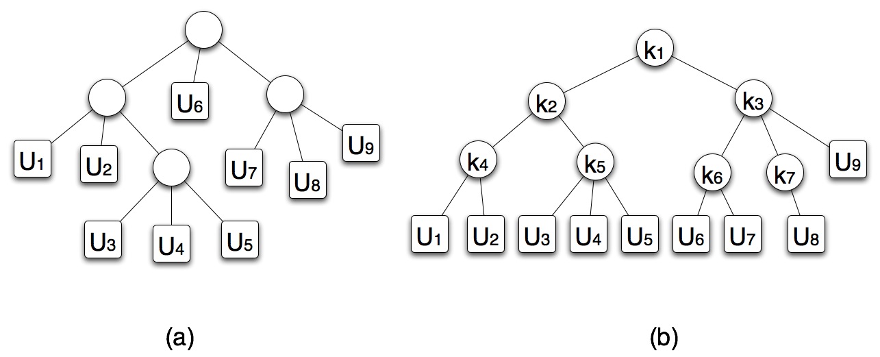
Figure 1: An instance of the Key Hierarchy Problem with 9 group members, connected to the group controller by a tree given in (a). Suppose the update frequency of every group member is 1 and the cost of every edge in the routing tree 1. An update at member $\mbox{U}_{4}$ will require the rekeying of keys $\mbox{K}_{5}$, $\mbox{K}_{2}$, and $\mbox{K}_{1}$. Key $\mbox{K}_{5}$ is rekeyed by unicasting to members $\mbox{U}_{3}$, $\mbox{U}_{4}$ and $\mbox{U}_{5}$ at a cost of 3 each. Key $\mbox{K}_{2}$ is rekeyed by multicasting to $\{\mbox{U}_{1},\mbox{U}_{2}\}$ and to $\{\mbox{U}_{3},\mbox{U}_{4},\mbox{U}_{5}\}$ at a cost of 3 and 5, respectively. Finally, key $\mbox{K}_{1}$ is rekeyed by multicasting to $\{\mbox{U}_{1},\mbox{U}_{2},\mbox{U}_{3},\mbox{U}_{4},\mbox{U}_{5}\}$, to $\{\mbox{U}_{6}\}$ and to $\{\mbox{U}_{7},\mbox{U}_{8},\mbox{U}_{9}\}$ at a cost of 7, 1, and 4, respectively. Thus, the total cost of an update at member $\mbox{U}_{4}$ is 29. Using similar calculations, the average cost of an update can be determined to be 219/9.

We introduce some notation that is useful for the remainder of the paper. We use $\mbox{OPT}(S)$ to denote the cost of an optimal hierarchy for $S$. We extend the notation $W$ to hierarchies and to sets of members: for any hierarchy $T$ (resp., set $X$ of members), $W(T)$ (resp., $W(X)$) denotes the sum of the weights of the leaves of $T$ (resp., members in $X$). Our algorithms often combine a set ${\cal H}$ of two or three hierarchies to form another hierarchy $T^{\prime}$: $\mbox{\tt combine}({\cal H})$ introduces a new root node $R$, makes the root of each hierarchy in ${\cal H}$ as a child of $R$, and returns the hierarchy rooted at $R$.

Using the above notation, a more convenient expression for the cost of a hierarchy $T$ over $X$ is the following reorganization of the summation in Equation 1:

$$\sum_{u\in T}W(T_{u})\sum_{\mbox{\scriptsize child }v\,\mbox{\scriptsize of }u}M(T_{v})$$ (2)

3 Uniform multicast cost

In this section, we consider the special case of the Key Hierarchy problem where the multicast cost to any subset of group members is the same. Thus, the objective is to minimize the average number of multicast messages sent for an update. We note that the number of multicast messages sent for an update at a member $u$ is simply the sum of the degrees of its ancestors in the hierarchy (as is evident from Equation 1). We start by establishing a basic structural property of an optimal hierarchy and a lower bound on the optimum cost.

Lemma 1

For any given member set $S$ with at least two members, there exists an optimal hierarchy in which the degree of every internal node is either two or three.

Proof

Let $T^{*}$ be an optimal hierarchy for $S$. Since any internal node with degree one can be replaced by its child, yielding a decrease in cost, the degree of every internal node of $T^{*}$ is at least two. Let, if possible, $v$ be an internal node of $T^{*}$ with degree $d\geq 4$. We divide its children into two groups $C_{1}$ and $C_{2}$, containing $\lceil d/2\rceil$ and $\lfloor d/2\rfloor$ children, respectively. We add two new internal nodes $v_{1}$ and $v_{2}$, make them children of $v$, and set $v_{1}$ and $v_{2}$ to be the parents of the nodes in $C_{1}$ and $C_{2}$, respectively.

We now consider the cost of the new hierarchy. The cost of any member that does not have $v$ as an ancestor in $T^{*}$ does not change. The cost of a member that has $v$ as an ancestor in $T^{*}$ decreases by at least $d-\lceil d/2\rceil-2\geq 0$; thus, this cost is nonincreasing. If $d>4$, there exists a member whose cost decreases by at least $d-\lfloor d/2\rfloor-2>0$, contradicting the optimality of $T^{*}$. If $d=4$, then we have a new hierarchy whose cost is no more than that of $T^{*}$ and has fewer internal nodes with degree greater than three. Repeating this process until there are no internal nodes with degree greater than 3 yields the desired claim.∎

Lemma 2

For any member set $S$, we have $\mbox{OPT}(S)\geq\sum_{v\in S}3w_{v}\log_{3}(W(S)/w_{v})$.

Proof

The proof is by induction on the size of $S$. The claim is trivially true for $|S|=1$. For the induction hypothesis, we assume that the claim is true for member sets of size less than $m\geq 2$. Consider an optimal hierarchy for $S$ with $|S|=m\geq 2$. Let the degree of the root be $d$, and let the member set in the subtree rooted at the $i$th child be $S_{i}$ with $|S_{i}|=m_{i}$, $1\leq i\leq d$. We place the following lower bound on $\mbox{OPT}(S)$:

$$\mbox{OPT}(S) \geq dW(S)+\sum_{1\leq i\leq d}\sum_{v\in S_{i}}3w_{i}\log_{3}(W(S_{i})/w_{v})$$

$$= dW(S)+3W(S)\sum_{1\leq i\leq d}\log_{3}W(S_{i})-\sum_{v\in S}3w_{v}\log_{3}w_{v}$$

$$\geq dW(S)+3W(S)\log_{3}(W(S)/d)-\sum_{v\in S}3w_{v}\log_{3}w_{v}$$

$$= dW(S)-3W(S)\log_{3}d+\sum_{v\in S}3w_{v}\log_{3}(W(S)/w_{v})$$

$$\geq \sum_{v\in S}3w_{v}\log_{3}(W(S)/w_{v}).$$

(The third step follows from the convexity of $x\log_{3}x$, the last step from $d\geq 3\log_{3}d$, $\forall d\geq 1$.)∎

3.1 Structure of an optimal hierarchy for uniform member weights

When all the members have the same weight, we can easily characterize an optimal key hierarchy by recursion. Let $n$ be the number of members. When $n=1$, the key hierarchy is just a single node tree. When $n=2$, the key hierarchy is a root with two leaves as children. When $n=3$, the key hierarchy is a root with three leaves as children. When $n>3$, we are going to build this key hierarchy recursively. First divide $n$ members into 3 balanced groups, i.e. the size of each group is between $\lfloor n/3\rfloor$ and $\lceil n/3\rceil$. Then the key hierarchy is a root with 3 children, each of which is the key hierarchy of one of the 3 groups built recursively by this procedure. It is easy to verify that the cost of this hierarchy is given by:

$$f(n)=\left\{\begin{array}[]{rl}3n\lfloor\log_{3}n\rfloor+4(n-k)&\mbox{when $k\leq n<2k$}\\ 3n\lfloor\log_{3}n\rfloor+5n-6k&\mbox{when $2k\leq n<3k$}\end{array}\right.$$

The following theorem is due to [9, 10], where this scenario arises as a special case of the constrained set selection problem. For completeness, we present an alternative shorter proof here.

Theorem 3.1 ([9, 10])

For uniform multicast costs and member weights, the above key hierarchy is optimal.

Proof

We prove this by induction on the number of members. Let $n$ be the number of members. For the base case ($n\leq 5$) we can check the optimality by brute-force. For inductive step ($n\geq 6$), we first make two observations: optimal key hierarchies have an optimal substructure property; and $f$ is a convex function of $n$.

By Lemma 1 we know there exists an optimal hierarchy in which the degree of the root is either two or three. We first consider the cse where the degree of the root is two. Since optimal key hierarchies satisfy the optimal substructure property, it must be the case that the sub-hierarchies rooted at the two children of the root must be optimal for the number of members in their respective subtrees. Thus, by the induction hypothesis, the cost of the optimal hierarchy equals $f(n_{1})+f(n-n_{1})+2n$, where $n_{1}$ is the number of members in the subtree rooted at one of the children of the root. Since $n\geq 6$, the convexity of $f$ implies that each subtree has at least 3 members. From the induction hypothesis, it also follows that the root of each subtree has degree 3. Let the two children of the root be $u_{1}$ and $u_{2}$. Let the children of $u_{i}$ be $u_{i1}$, $u_{i2}$, and $u_{i3}$, $1\leq i\leq 2$. We transform this hierarchy into another key hierarchy with the same cost by adding a third child $u_{3}$ to the root that has as its children $u_{13}$ and $u_{23}$. The cost of every member in the new hierarchy remains the same as that in the optimal hierarchy, which means this new hierarchy is also optimal and its root has degree 3.

So we now focus on the case where there exists an optimal hierarchy in which the root has degree 3. Let the three children of the root have $n_{1}$, $n_{2}$, and $n_{3}$ members, respectively. It follows that the cost of the optimal hierarchy equals $f(n_{1})+f(n_{2})+f(n_{3})+3n$. The convexity of $f$ implies that the preceding cost is minimized when each of $n_{1}$, $n_{2}$, and $n_{3}$ is either $\lfloor n/3\rfloor$ or $\lceil n/3\rceil$. This is precisely the proposed hierarchy, thus completing the proof of the theorem.∎

3.2 A polynomial-time approximation scheme for nonuniform member weights

We give a polynomial-time approximation scheme for the Key Hierarchy Problem when the multicast cost to every subset of the group is identical and the members have arbitrary weights. Given a positive constant $\varepsilon$, we present an polynomial-time algorithm that produces a $(1+O(\varepsilon))$-approximation. We assume that $1/\varepsilon$ is a power of 3; if not, we can replace $\varepsilon$ by a smaller constant that satisfies this condition. We round the weight of every member up to the nearest power of $(1+\varepsilon)$ at the expense of a factor of $1+\varepsilon$ in approximation. Thus, in the remainder we assume that every weight is a power of $(1+\varepsilon)$. Our algorithm $\mbox{PTAS}(S)$, which takes as input a set $S$ of members with weights, is as follows.

• Divide $S$ into two sets, a set $H$ of the $3^{1/\varepsilon^{2}}$ members with the largest weight and the set $L=S-H$.

• Initialize ${\cal L}$ to be the set of hierarchies consisting of one depth-0 hierarchy for each member of $L$.

• Repeat the following step until it can no longer be executed: if $T_{1}$, $T_{2}$, and $T_{3}$ are hierarchies in ${\cal L}$ with identical weight, then replace $T_{1}$, $T_{2}$, and $T_{3}$ in ${\cal L}$ by $\mbox{\tt combine}(\{T_{1},T_{2},T_{3}\})$. (Recall the definition of combine from Section 2.)

• Repeat the following step until ${\cal L}$ has one hierarchy: replace the two hierarchies $T_{1}$, $T_{2}$ with least weight by $\mbox{\tt combine}(\{T_{1},T_{2}\})$. Let $T_{L}$ denote the hierarchy in ${\cal L}$.

• Compute an optimal hierarchy $T^{*}$ for $H$. Determine a node in $T^{*}$ that has weight at most $W(S)\varepsilon$ and height at most $1/\varepsilon$. We note that such a node exists since every hierarchy with at least $\ell$ leaves has a set $N$ of at least $1/\varepsilon$ nodes at depth at most $1/\varepsilon$ with the property that no node in $N$ is an ancestor of another. Set the root of $T_{L}$ as the child of this node. Return $T^{*}$.

We now analyze the above algorithm. At the end of step 3, the cost of any hierarchy $T$ in ${\cal L}$ is equal to $\sum_{v\in T}3w_{v}\log_{3}(W(T)/w_{v})$. If ${\cal L}$ is the hierarchy set at the end of step 3, then the additional cost incurred in step 4 is at most $\sum_{T\in{\cal L}}2W(T)\log_{2}(W(L)/W(T))$.

Since there are at most two hierarchies in any weight category in ${\cal L}$ at the start of step 4, at least $1-1/\varepsilon^{2}$ of the weight in the hierarchy set is concentrated in the heaviest $4/\varepsilon^{3}$ hierarchies of ${\cal L}$. Step 4 is essentially the Huffman coding algorithm and yields an optimal binary hierachy. Using Lemma 3 of Section 5, we note that it achieves a $3$-approximation. (In fact, one can show using a more careful argument that it achieves an approximation of $2\lg((1+\sqrt{5})/2)/(3\lg 3)\approx 1.52$, but the factor 3 will suffice for our purposes here.) This yields the following bound on the increase in cost due to step 4:

$$3\left(\varepsilon^{2}W(L)\log_{1+\varepsilon}3+(1-\varepsilon^{2})W(L)\log_{2}(4/\varepsilon^{2})\right)\leq W(L)/\varepsilon,$$

for $\varepsilon$ sufficiently small. The final step of the algorithm increases the cost by at most $W(L)/\varepsilon+\varepsilon W(S)$. Thus, the total cost of the final hierarchy is at most

$$\mbox{OPT}(H)+\mbox{OPT}(L)+W(L)/\varepsilon+W(L)/\varepsilon+\varepsilon W(S)$$

$$\leq \mbox{OPT}(H)+\mbox{OPT}(L)+2\varepsilon\mbox{OPT}(S)+\varepsilon\mbox{OPT}(S)$$

$$\leq (1+3\varepsilon)\mbox{OPT}(S).$$

(The second step holds since $\mbox{OPT}(S)\geq\sum_{v\in L}w_{v}\log_{3}(W(S)/w_{v})\geq W(L)/\varepsilon^{2}$.)

4 Hardness results

In this section, we present the hardness results for Key Hierarchy Problem with nonuniform multicast cost. First we show that the problem is strongly NP-complete if group members have different weights and the underlying routing network is a tree. Then we show the problem is also NP-complete if group members have the same weights and the underlying routing network is a general graph.

4.1 Weighted key hierarchy problem with routing tree

Our reduction is from the NP-complete problem 3-Partition, which is defined as follows [5]. The input consists of a set $A$ of $3m$ elements, a bound $B\in Z^{+}$, and a set of sizes $S(a)\in Z^{+}$ for each $a\in A$ such that $B/4<S(a)<B/2$, and $\sum_{a\in A}S(a)=mB$. The goal of the problem is to determine whether $A$ can be partitioned into $m$ disjoint sets $A_{1},A_{2},\dots,A_{m}$ such that for $1\leq i\leq m$, $\sum_{a\in A_{i}}S(a)=B$.

Theorem 4.1

When group members have different weights and the routing network is a tree, the Key Hierarchy Problem is NP-complete.

Proof

The membership in NP is immediate. We reduce 3-partition to the Key Hierarchy Problem. Let $P$ denote the given 3-Partition instance. If the number $3m$ of elements in the $P$ is not a power of three, then we add new elements in groups of three with sizes $B$, $0$, and $0$, respectively, to make the total number of elements a power of 3. It is easy to verify that the original problem instance has the desired partition if and only if the new instance has the desired partition. Thus, for the remainder of the proof, we assume that the number of elements, $3m$, in $P$ is a power of $3$.

In $P$, let set $A$ be $\{a_{1},a_{2},\dots,a_{3m}\}$, and the size of element $a_{i}$ in set $A$ be $w^{\prime}_{i}$. We create a routing tree $T$ consisting of a root $r$ connected to a single internal node $u$, which in turn has edges to $3m$ leaves $v_{i}$ for $i=1,2,\dots,3m$, one for each of the $3m$ members. Root $r$ is the group controller. For member $i$, we set its weight $w_{i}$ to be $w+w^{\prime}_{i}$, where $w$ is chosen such that $\frac{w_{max}}{w_{min}}<\frac{3\cdot 3m\log_{3}3m+1}{3\cdot 3m\log_{3}3m}$, where $w_{max}=\max_{i}\{w_{i}\}$ and $w_{min}=\min_{i}\{w_{i}\}$. We set the cost of edge $(r,u)$ to be $C$, a constant which will be specified later, and the cost of $(u,v_{i})$ to be $w_{i}$ for $i=1,2,\dots,3m$, and the weight of leaf $v_{i}$ to be $w_{i}$. We now show that $P$ has a partition if and only if the optimal key hierarchy of $T$ has cost $C\cdot 3W\log_{3}3m+W^{2}\cdot\left(1+1/3+1/9+\dots+1/m\right)$, where $W$ is the sum of the weights of all the members.

If we set $C>W^{2}\log_{3}3m$, then the cost of an optimal key hierarchy is smaller than $C\cdot 3\cdot 3m\log_{3}3m\cdot w_{max}$, which is the optimal cost for $3m$ members, each with weight $w_{max}$. In an optimal key hierarchy, every internal node has degree 3, since otherwise its cost is at least $C\cdot\left(3\cdot 3m\log_{3}3m+1\right)\cdot w_{min}$, which is not optimal given that $\frac{w_{max}}{w_{min}}<\frac{3\cdot 3m\log_{3}3m+1}{3\cdot 3m\log_{3}3m}$. So, a balanced degree-3 tree is the only optimal key hierarchy in this case. In such a hierarchy, the cost contributed by edge $(r,u)$ is exactly $C\cdot 3W\log_{3}3m$. Let $C_{i}$ denote the set of nodes at depth $i$ in the hierarchy, the depth of the root being set to $0$. By Equation 2, the cost contributed by edges $(u,v_{i})$, $i=1,2,\dots,3m$, equals

$$\sum_{0\leq i\leq\log_{3}m}\sum_{x\in C_{i}}W(T_{x})\cdot(M(T_{x})-C)$$

$$= \sum_{0\leq i\leq\log_{3}m}\sum_{x\in C_{i}}W(T_{x})^{2}$$

$$\geq W^{2}+3(W/3)^{2}+9(W/9)^{2}+\dots+m(W/m)^{2}.$$

In the last step, equality only holds when $W(T_{x})=W/3^{i}$ for all $x\in C_{i}$ (by Jensen’s inequality). Thus, the 3-partition problem has a solution if and only if the optimal key hierarchy achieves its minimum, which is $C\cdot 3W\log_{3}3m+W^{2}\cdot\left(1+1/3+1/9+\dots+1/m\right)$.∎

4.2 Unweighted key hierarchy problem

Our reduction is from the NP-complete 3D-Matching problem which is defined as follows [5]. We are given finite disjoint sets $W,U,V$ of size $q$, and a set of triples $M\subseteq W\times U\times V$. The goal is to determine whether there are $q$ pairwise disjoint triples.

Theorem 4.2

When group members have the same key update weights and the routing network is a general graph, the Key Hierarchy Problem is NP-complete.

Proof

We reduce 3D-Matching to the Key Hierarchy problem. Let $I$ be a given instance of 3D-Matching. If the set size $q$ is not a power of 3 and $q^{\prime}$ is the smallest power of 3 larger than $q$, then we construct a new instance of 3D-Matching by adding $q^{\prime}-q$ new elements to each of $W$, $U$, and $V$ as follows: for $1\leq i\leq q^{\prime}-q$, add $w^{\prime}_{i}$ to $W$, $u^{\prime}_{i}$ to $U$, $v^{\prime}_{i}$ to $V$, and $(w^{\prime}_{i},u^{\prime}_{i},v^{\prime}_{i})$ to $M$. It is easy to see that the original 3D-Matching instance has a solution if and only if this new 3D-Matching instance has a solution. So from now on we can assume that $q$ is a power of 3.

For given instance $I$, we construct a routing graph as follows. Create vertices $w_{1},w_{2},\dots,w_{q}$ to represent each element in set $W$, $u_{1},u_{2},\dots,u_{q}$ to represent each element in set $U$, and $v_{1},v_{2},\dots,v_{q}$ to represent each element in set $V$. Then create $|M|$ vertices $t_{1},t_{2},\dots,t_{|M|}$, and for each element $m_{i}=(w_{x},u_{y},v_{z})\in M$, add edges $(t_{i},w_{x}),(t_{i},u_{y}),(t_{i},v_{z})$ of unit cost to the routing graph. Create another vertex $s$, and add edges $(s,t_{i})$ for $i=1,2,\dots,|M|$ of unit cost. Finally, create vertex $r$, and add an edge $(r,s)$ with cost $c$. Vertex $r$ is the group controller, and $W\cup U\cup V$ is the set of group members.

If we set $c$ to be greater than $(|M|+3q)\cdot 3\cdot 3q\log_{3}3q$, then using an argument similar to the proof of Theorem 4.1, we can show that the optimal key hierarchy is a balanced degree-3 tree. We will next argue that there is a matching in $I$ if and only if the cost of the optimal key hierarchy is $c\cdot 3\cdot 3q\log_{3}3q+6q(3q-1)$.

We now calculate the cost of the optimal hierarchy using Equation 2. The cost contributed by edge $(r,s)$ is exactly $c\cdot 3\cdot 3q\log_{3}3q$. The cost contributed by edges $(t_{i},w_{x})$, $(t_{i},u_{y})$ and $(t_{i},v_{z})$ where $i=1,2,\dots,|M|$ and $x,y,z=1,2,\dots,q$, is $\frac{9}{2}q(3q-1)$. The cost contributed by edges $(s,t_{i})$, $i=1,2,\dots,|M|$, is at least $\frac{3}{2}q(3q-1)$. This minimum is achieved only if there is a 3D-Matching. So there is a solution to the 3D-Matching problem if and only if the cost of the optimal logical tree is $c\cdot 3\cdot 3q\log_{3}3q+6q(3q-1)$. And this completes the proof of the theorem. ∎

5 Approximation algorithms for nonuniform multicast costs

In this section, we present constant-factor approximation algorithms for the Key Hierarchy Problem with nonuniform multicast costs. We first show that for any instance, there always exists a binary hierarchy that is 3-approximate. This guides the design of our approximation algorithms. We next present, in Section 5.1, an 11-approximation algorithm for the case where the underlying communication network is a tree. Finally, we present, in Section 5.2 a 75-approximation algorithm for the most general case of our problem, where the communication network is an arbitrary weighted graph.

Lemma 3

For any instance, there exists a 3-approximate binary hierarchy.

Proof

Consider any optimal hierarchy $T$. Following Equation 2, we associate with each node $u$ of $T$ a cost equal to $W(T_{u})\sum_{\mbox{\scriptsize child }v\mbox{ of }u}M(T_{v})$; we refer to this cost as $\mbox{nc}(u)$. We show how to transform $T$ to a binary hierarchy by repeatedly replacing a node, say $u$, with degree $d\geq 2$, by a node $u^{\prime}$ of degree two and a set $U$ of at most two other nodes, each with degree strictly less than $d$. To argue the bound on the cost of the binary hierarchy, we use a charging argument: in particular, we show that $3\mbox{nc}(u)\geq\mbox{nc}(u^{\prime})+\sum_{v\in U}3\mbox{nc}(v)$.

Consider any node $u$ of $T$ of degree greater than two. We consider two cases. The first case is where there is no child of $u$ that has weight at least one-third of the weight under $u$. We divide the children of $u$ into two groups such that each group has at least one-third of weight under $u$. If such a partition exists, then we replace $u$ by three nodes: $u^{\prime}$, $u_{1}$, and $u_{2}$. The parent of node $u^{\prime}$ is the same as the parent of $u$ (if it exists). The node $u^{\prime}$ is the parent for both $u_{1}$ and $u_{2}$. Finally, $u_{1}$ and $u_{2}$ are the parents of the children of $u$ in the two groups of the partition, respectively.

$$3\mbox{nc}(u) = 3W(T_{u})\sum_{\mbox{\scriptsize child }v\mbox{ of }u}M(T_{v})$$

$$\leq W(T_{u})(M(T_{u_{1}})+M(T_{u_{2}}))+2W(T_{u})\sum_{\mbox{\scriptsize child }v\mbox{ of }u}M(T_{v})$$

$$= \mbox{nc}(u^{\prime})+2W(T_{u})\sum_{\mbox{\scriptsize child }v\mbox{ of }u_{1}}M(T_{v})+2W(T_{u})\sum_{\mbox{\scriptsize child }v\mbox{ of }u_{2}}M(T_{v})$$

$$\leq \mbox{nc}(u^{\prime})+3\mbox{nc}(u_{1})+3\mbox{nc}(u_{2}).$$

The second case is where $u$ has a child $u_{1}$ with weight at least two-third of the total weight under $u$. In this case, we replace $u$ by two nodes $u^{\prime}$ and $u_{2}$, with $u^{\prime}$ becoming the parent of $u_{1}$ and $u_{2}$, and $u_{2}$ becoming the parent of the other children of $u$. The parent of $u^{\prime}$ is the same as that of $u$ (if it exists). Using a similar argument as above, we obtain that $3\mbox{nc}(u)$ equals $3W(T_{u})\sum_{\mbox{\scriptsize child }v\mbox{ of }u}M(T_{v})$, which is at most $\mbox{nc}(u^{\prime})+3\mbox{nc}(u_{2})$.∎

5.1 Approximation algorithms for routing trees

In this section, we first give an 11-approximation algorithm for the case where weights are nonuniform and the routing network is a tree. Then we analyze the more special case with uniform weights, and improve the approximation factor to 4.2.

Given any routing tree, let $S$ be the set of members. We start with defining a procedure $\mbox{\tt partition}(\cdot)$ that takes as input the set $S$ and returns a pair $(X,v)$ where $X$ is a subset of $S$ and $v$ is a node in the routing tree. First, we determine if there is an internal node $v$ that has a subset $C$ of children such that the total weight of the members in the subtrees of the routing tree rooted at the nodes in $C$ is between $W(S)/3$ and $2W(S)/3$. If $v$ exists, then we partition $S$ into two parts $X$, which is the set of members in the subtrees rooted at the nodes in $C$, and $S\setminus X$. It follows that $W(S)/3\leq W(X)\leq 2W(S)/3$. If $v$ does not exist, then it is easy to see that there is a single member with weight more than $2W(S)/3$. In this case, we set $X$ to be the singleton set which contains this heavy node which we call $v$. The procedure $\mbox{\tt partition}(S)$ returns the pair $(X,v)$. In the remainder, we let $Y$ denote $S\setminus X$.

ApproxTree($S$)

• If $S$ is a singleton set, then return the trivial hierarchy with a single node.

• $(X,v)=\mbox{\tt partition}(S)$; let $Y$ denote $S\setminus X$.

• Let $\Delta$ be the cost from root to partition node $v$. If $\Delta\leq M(S)/5$, then let $T_{1}=$ApproxTree($X$); otherwise $T_{1}=\mbox{PTAS}(X)$. (PTAS is the algorithm introduced in Section 3.2.)

• $T_{2}=$ApproxTree($Y$).

• Return $\mbox{\tt combine}(T_{1},T_{2})$.

Theorem 5.1

Algorithm ApproxTree is an $(11+\varepsilon)$-approximation, where $\varepsilon>0$ can be made arbitrarily small.

Proof

Let $\mbox{ALG}(S)$ be the key hierarchy constructed by our algorithm, $\mbox{OPT}(S)$ be the optimal key hierarchy. In the following proof, we abuse our notation and use $\mbox{ALG}(\cdot)$ and $\mbox{OPT}(\cdot)$ to refer to both the key hierarchies and their cost. We first note that $\mbox{OPT}(S)\geq\mbox{OPT}(X)+\mbox{OPT}(Y)$.

We prove by induction on the number of members in $S$ that $\mbox{ALG}(S)\leq\alpha\cdot\mbox{OPT}(S)+\beta\cdot W(S)M(S)$, for constants $\alpha$ and $\beta$ specified later. The induction base, when $|S|\leq 2$, is trivial. For the induction step, we consider three cases depending on the distance to the partition node and whether we obtain a balanced partition; we say that a partition $(X,Y)$ is balanced if $\frac{1}{3}W(S)\leq W(X),W(Y)\leq\frac{2}{3}W(S)$. The first case is where $\Delta\leq M(S)/5$ and the partition is balanced. In this case, we have

$$\mbox{ALG}(S) = \mbox{ALG}(X)+\mbox{ALG}(Y)+W(S)\left[M(X)+M(Y)\right]$$

$$\leq \alpha\cdot\mbox{OPT}(X)+\beta\cdot W(X)M(X)+\alpha\cdot\mbox{OPT}(Y)+\beta\cdot W(Y)M(Y)$$

$$+W(S)\left[M(X)+M(Y)\right]$$

$$\leq \alpha\left[\mbox{OPT}(X)+\mbox{OPT}(Y)\right]+\left(\frac{2}{3}\beta+1\right)W(S)\left[M(X)+M(Y)\right]$$

$$\leq \alpha\cdot\mbox{OPT}(S)+\left(\frac{2}{3}\beta+1\right)W(S)\left[M(S)+\Delta\right]$$

$$\leq \alpha\cdot\mbox{OPT}(S)+\frac{6}{5}\left(\frac{2}{3}\beta+1\right)w(S)M(S)$$

$$\leq \alpha\cdot OPT(S)+\beta\cdot w(S)M(S)$$

as long as $\frac{6}{5}\left(\frac{2}{3}\beta+1\right)\leq\beta$, which is true if $\beta\geq 6$. The second case is where $\Delta>M(S)/5$ and the partition is balanced. In this case, we only call the algorithm recursively on $Y$ and use PTAS on $X$.

$$\mbox{ALG}(S) = \mbox{PTAS}(X)+\mbox{ALG}(Y)+W(S)\left[M(X)+M(Y)\right]$$

$$\leq 5(1+\varepsilon)\cdot\mbox{OPT}(X)+\alpha\cdot\mbox{OPT}(Y)+\beta\cdot W(Y)M(Y)$$

$$+W(S)\left[M(X)+M(Y)\right]$$

$$\leq \alpha\left[\mbox{OPT}(X)+\mbox{OPT}(Y)\right]+\frac{2}{3}\beta W(S)M(S)+2W(S)M(S)$$

$$\leq \alpha\cdot\mbox{OPT}(S)+\left(\frac{2}{3}\beta+2\right)W(S)M(S)$$

$$\leq \alpha\cdot\mbox{OPT}(S)+\beta\cdot W(S)M(S)$$

as long as $\alpha\geq 5(1+\varepsilon)$ and $\frac{2}{3}\beta+2\leq\beta$ which is true if $\beta\geq 6$. The third case is when the partition is not balanced (i.e. $W(X)>\frac{2}{3}W(S)$). In this case, our algorithm connects the heavy node directly to the root of the hierarchy.

$$\mbox{ALG}(S) = \mbox{ALG}(Y)+W(S)\left[M(X)+M(Y)\right]$$

$$\leq \alpha\cdot\mbox{OPT}(Y)+\beta\cdot W(Y)M(Y)+W(S)\left[M(X)+M(Y)\right]$$

$$\leq \alpha\cdot\mbox{OPT}(S)+\frac{1}{3}\beta W(S)M(S)+2W(S)M(S)$$

$$\leq \alpha\cdot\mbox{OPT}(S)+\left(\frac{1}{3}\beta+2\right)W(S)M(S)$$

$$\leq \alpha\cdot\mbox{OPT}(S)+\beta\cdot W(S)M(S)$$

as long as $\frac{1}{3}\beta+2\leq\beta$ which is true if $\beta\geq 3$. So, by induction, we have shown $\mbox{ALG}(S)\leq\alpha\cdot\mbox{OPT}(S)+\beta\cdot W(S)M(S)$ for $\alpha\geq 5(1+\varepsilon)$ and $\beta\geq 6$. Since $\mbox{OPT}(S)\geq W(S)M(S)$, we obtain an $(11+\varepsilon)$-approximation.∎

If the member weights are uniform, then we can improve the approximation ratio to 4.2 using a more careful analysis of the same algorithm. We refer the reader to the appendix for details.

5.2 Approximation algorithms for routing graphs

In this section, we give a constant-factor approximation algorithm for the case where weights are nonuniform and the routing network is an arbitrary graph. In our algorithm, we compute light approximate shortest-path trees (LAST) [14] of subgraphs of the routing graph. An $(\alpha,\beta)$-LAST of a given weighted graph $G$ is a spanning tree $T$ of $G$ such that the the shortest path in $T$ from a specified root to any vertex is at most $\alpha$ times the shortest path from the root to the vertex in $G$, and the total weight of $T$ is at most $\beta$ times the minimum spanning tree of $G$. For any $\gamma>0$, the algorithm of [14] yields a an $(\alpha,\beta)$-LAST with $\alpha=1+\sqrt{2}\gamma$ and $\beta=1+\sqrt{2}/\gamma$, where $\gamma$ can be chosen as an input parameter.

ApproxGraph($S$)

• If $S$ is a singleton set, return the trivial hierarchy with one node.

• Compute the complete graph on $S\cup\{root\}$. The weight of an edge $(u,v)$ is the length of shortest path between $u$ and $v$ in the original routing graph.

• Compute the minimum spanning tree on this complete graph. Call it MST($S$).

• Compute an $(\alpha,\beta)$-LAST $L$ of MST($S$).

• $(X,v)=\mbox{\tt partition}(L)$.

• Let $\Delta$ be the cost from root to partition node $L$. If $\Delta\leq M(S)/5$, then let $T_{1}=$ApproxGraph($X$). Otherwise, $T_{1}=\mbox{PTAS}(X)$.

• $T_{2}=$ApproxGraph($Y$).

• Return $\mbox{\tt combine}(T_{1},T_{2})$.

The optimum multicast to a member set is obtained by a minimum Steiner tree, computing which is NP-hard. It is well known that the minimum Steiner tree is 2-approximated by a minimum spanning tree (MST) in the metric space connecting the root to the desired members (the metric being the shortest path cost in the routing graph). So at the cost of a factor 2 in the approximation, we define $M(S)$ to be the cost of the MST connecting the root to $S$ in the complete graph $G(S)$ whose vertex set is $S\cup\{root\}$ and the weight of edge $(u,v)$ is the shortest path distance between $u$ and $v$ in the routing graph.

Theorem 5.2

The algorithm ApproxGraph is a constant-factor approximation.

Proof

We prove by induction on the number of members in $S$ that $\mbox{ALG}(S)\leq\alpha\cdot\mbox{OPT}(S)+\beta\cdot W(S)M(S)$, for constants $\alpha$ and $\beta$ specified later. The induction base, when $|S|\leq 2$, is trivial. For the induction step, we consider three cases. The first case is $\Delta\leq M(S)/5$ and the partition is balanced (as defined in the proof of Theorem 5.1). Let $M_{L}(S)$ be the multicast cost to $S$ in LAST. From the description of LAST we know $M_{L}(S)\leq\left(1+\sqrt{2}/\gamma\right)\cdot M(S)$. Also we have $M_{L}(S)\geq M_{L}(X)+M_{L}(Y)-\Delta\geq M(X)+M(Y)-\Delta$. So $\left(1+\sqrt{2}/\gamma\right)\cdot M(S)\geq M(X)+M(Y)-\Delta$.

$$\mbox{ALG}(S) = \mbox{ALG}(X)+\mbox{ALG}(Y)+W(S)\left[M(X)+M(Y)\right]$$

$$\leq \alpha\cdot\mbox{OPT}(X)+\beta\cdot W(X)M(X)+\alpha\cdot\mbox{OPT}(Y)+\beta\cdot W(Y)M(Y)$$

$$+W(S)\left[M(X)+M(Y)\right]$$

$$\leq \alpha\left[\mbox{OPT}(X)+\mbox{OPT}(Y)\right]+\left(\frac{2}{3}\beta+1\right)W(S)\left[M(X)+M(Y)\right]$$

$$\leq \alpha\cdot\mbox{OPT}(S)+\left(\frac{2}{3}\beta+1\right)W(S)\left[\left(1+\sqrt{2}/\gamma\right)M(S)+\Delta\right]$$

$$\leq \alpha\cdot\mbox{OPT}(S)+\left(\frac{6}{5}+\sqrt{2}/\gamma\right)\left(\frac{2}{3}\beta+1\right)W(S)M(S)$$

$$\leq \alpha\cdot OPT(S)+\beta\cdot W(S)M(S)$$

as long as $\left(\frac{6}{5}+\sqrt{2}/\gamma\right)\left(\frac{2}{3}\beta+1\right)\leq\beta$.

The second case is $\Delta>M(S)/5$ and the partition is balanced. In this case, we only call the algorithm recursively on $Y$ and use the PTAS for $X$. Since $\Delta>M(S)/5$, the distance from the root to any element in $X$ is at least $\frac{\Delta}{1+\sqrt{2}\gamma}=\frac{M(S)}{5(1+\sqrt{2}\gamma)}$. So the multicast cost to any subset of $X$ is between $\frac{M(S)}{5(1+\sqrt{2}\gamma)}$ and $M(S)$. By using the PTAS, we have a $5(1+\varepsilon)(1+\sqrt{2}\gamma)$-approximation on $\mbox{OPT}(X)$. So we have the following bound on $\mbox{ALG}(S)$.

$$\mbox{ALG}(S) = \mbox{PTAS}(X)+\mbox{ALG}(Y)+W(S)\left[M(X)+M(Y)\right]$$

$$\leq 5\left(1+\sqrt{2}\gamma\right)(1+\varepsilon)\cdot\mbox{OPT}(X)+\alpha\cdot\mbox{OPT}(Y)+\beta\cdot W(Y)M(Y)$$

$$+W(S)\left[M(X)+M(Y)\right]$$

$$\leq \alpha\left[\mbox{OPT}(X)+\mbox{OPT}(Y)\right]+\frac{2}{3}\beta W(S)M(S)+2W(S)M(S)$$

$$\leq \alpha\cdot\mbox{OPT}(S)+\left(\frac{2}{3}\beta+2\right)W(S)M(S)$$

$$\leq \alpha\cdot\mbox{OPT}(S)+\beta\cdot W(S)M(S)$$

as long as $\alpha\geq 5\left(1+\sqrt{2}\gamma\right)(1+\varepsilon)$ and $\beta\geq 6$.

The third case is when the partition is not balanced. In this case, our algorithm connect the heavy node directly to the root of key hierarchy. So we have the following bound on $\mbox{ALG}(S)$.

$$\mbox{ALG}(S) = \mbox{ALG}(Y)+W(S)\left[M(X)+M(Y)\right]$$

$$\leq \alpha\cdot\mbox{OPT}(Y)+\beta\cdot W(Y)M(Y)+W(S)\left[M(X)+M(Y)\right]$$

$$\leq \alpha\cdot\mbox{OPT}(S)+\frac{1}{3}\beta W(S)M(S)+2W(S)M(S)$$

$$\leq \alpha\cdot\mbox{OPT}(S)+\left(\frac{1}{3}\beta+2\right)W(S)M(S)$$

$$\leq \alpha\cdot\mbox{OPT}(S)+\beta\cdot W(S)M(S)$$

as long as $\beta\geq 3$. So, this algorithm has a constant approximation.

So, by induction, we have shown $\mbox{ALG}(S)\leq\alpha\cdot\mbox{OPT}(S)+\beta\cdot W(S)M(S)$, implying an $(\alpha+\beta)$-approximation. When $\gamma=7$, from the constraints, we obtain $\alpha\geq 54$ and $\beta\geq 21$. So we have a $75$-approximation.∎

6 Discussion

We have presented a constant-factor approximation algorithm for the Key Hierarchy Problem for the general case where the member weights are nonuniform and the communication network is an arbitrary graph. While we do obtain improved approximation factors when the communication network is a tree, the factors achieved are large and need to be improved. We have also given a polynomial-time approximation scheme for the problem instance where all multicasts cost the same. We do not know, however, whether this problem is NP-complete. As discussed in Section 1.2, the problem is related to the classic Huffman coding problem with nonuniform letter costs, whose complexity (P vs NP-hardness) is also not yet resolved.

There are several other directions for future research. We are currently exploring the dynamic maintenance of our key hierarchies, explicitly modeling the joining and leaving of members, while maintaining the constant-factor approximation in cost. We would also like to study the design of key hierarchies where the members have a bound on the number of auxiliary keys they store. Also of interest is the case where we have no (or limited) information on the update frequencies of the members.

Appendix 0.A Improved approximation for the routing tree case when weights are uniform

For the case where group members have the same key update probability and the communication network is a tree, using the same algorithm we can show the approximation ratio is 4.2 by a different analysis, shown as follows.

Claim

Balanced partition node can always be found if the members have the same key update weight.

Proof

Suppose this kind of partition node doesn’t exist, which means for all internal node $v$, its number of leaves is either $<n/3$ or $>2n/3$. We call nodes with less than $n/3$ leaves small nodes, and nodes with more than $2n/3$ leaves large nodes. Consider the large node with only small nodes as its children, there must be a combination of its children whose total number of leaves is between $n/3$ and $2n/3$. This means this kind of partition node exists.∎

Lemma 4

$\mbox{ALG}(S)\leq\mbox{ALG}(X)+\mbox{ALG}(Y)+\frac{4\Delta}{3\log 3/2}n\log n+n\left(M(X)+M(Y)\right)$.

Proof

(1) The cost of nodes in $\mbox{ALG}(Y)$ is the same as their cost in $\mbox{ALG}(S)$. (2) Similarly, the cost of nodes in $\mbox{ALG}(X)$ is equal to their cost in $\mbox{ALG}(S)+\frac{4\Delta}{3\log 3/2}n\log n$. The reason we add $\frac{4\Delta}{3\log 3/2}n\log n$ is the multicast cost of each node in $\mbox{ALG}(X)$ increased by $\Delta$ compared to its cost in $\mbox{ALG}(X)$. Since in the worst case $\mbox{ALG}(X)$ has $\log_{\frac{3}{2}}\frac{n}{3}$ levels, the increased cost is at most $2|X|\Delta\log_{\frac{3}{2}}\frac{n}{3}\leq 2\frac{2n}{3}\Delta\log_{\frac{3}{2}}\frac{n}{3}\leq\frac{4\Delta}{3\log 3/2}n\log n$. Combine (1) and (2), then add the cost of the root of $\mbox{ALG}(X)$ and $\mbox{ALG}(Y)$, we know this lemma is correct.∎

Lemma 5

$\mbox{OPT}(S)\geq\mbox{OPT}(X)+\mbox{OPT}(Y)+\frac{3\Delta}{\log 3}n\log n$

Proof

To any subset of $X$, the multicast cost calculated in $\mbox{OPT}(S)$ is $\Delta$ more than the cost calculated in $\mbox{OPT}(X)$. From Theorem 3.1, we know the increased cost is at least $3\Delta\cdot n\log_{3}n=\frac{3\Delta}{\log 3}n\log n$.∎

Theorem 0.A.1

This is a 4.2-approximation algorithm.

Proof

$$\mbox{ALG}(S)$$

$$\leq \mbox{ALG}(X)+\mbox{ALG}(Y)+\frac{4\Delta}{3\log 3/2}n\log n+n\left(M(X)+M(Y)\right)$$

$$\leq \alpha\cdot\mbox{OPT}(X)+\beta\cdot|X|M(X)+\alpha\cdot\mbox{OPT}(Y)+\beta\cdot|Y|M(Y)+\frac{4\Delta}{3\log 3/2}n\log n$$

$$+n\left(M(X)+M(Y)\right)$$

$$\leq \alpha\left[\mbox{OPT}(X)+\mbox{OPT}(Y)\right]+\frac{4\Delta}{3\log 3/2}n\log n+\left(\frac{2}{3}\beta+1\right)n\left(M(X)+M(Y)\right)$$

$$\leq \alpha\left[\mbox{OPT}(S)-\frac{3\Delta}{\log 3}n\log n\right]+\frac{4\Delta}{3\log 3/2}n\log n+\left(\frac{2}{3}\beta+1\right)n\left(M(X)+M(Y)\right)$$

$$\leq \alpha\left[\mbox{OPT}(S)-\frac{3\Delta}{\log 3}n\log n\right]+\dfrac{4\Delta}{3\log 3/2}n\log n+\left(\frac{2}{3}\beta+1\right)n\left(M(S)+\Delta\right)$$

$$= \alpha\cdot\mbox{OPT}(S)+\left(\frac{2}{3}\beta+1\right)nM(S)-\alpha\cdot\frac{3\Delta}{\log 3}n\log n+\frac{4\Delta}{3\log 3/2}n\log n$$

$$\leq \alpha\cdot\mbox{OPT}(S)+\beta\cdot nM(S)$$

as long as $\alpha\geq 1.2$ and $\beta\geq 3$. This means this is a 4.2-approximation.∎

References

- [1] Awerbuch, B., Baratz, A.E., Peleg, D.: Cost-Sensitive Analysis of Communication Protocols. In: PODC (1990)
- [2] Canetti, R., Garay, J., Itkis, G., Micciancio, D., Naor, M., Pinkas, B.: Multicast Security: A Taxonomy and Some Efficient Constructions. In: INFOCOMM (1999)
- [3] Canetti, R., Malkin, T., Nissim, K.: Efficient Communication-Storage Tradeoffs for Multicast Encryption. In: EUROCRYPT (1999)
- [4] Caronni, G., Waldvogel, M., Sun, D., Plattner, B.: Efficient Security for Large and Dynamic Multicast Groups. In: WETICE (1998)
- [5] Garey, M. R., Johnson, D. S.: Computers and Intractability: A Guide to the Theory of NP-Completeness. Freeman, New York (1979)
- [6] Golin, M.J., Kenyon, C., Young, N.E.: Huffman coding with unequal letter costs. In: STOC (2002)
- [7] Harney, H., Muckenhirn, C.: Group Key Management Protocol (GKMP) Architecture. Internet RFC 2094 (1997)
- [8] Harney, H., Muckenhirn, C.: Group Key Management Protocol (GKMP) Specification. Internet RFC 2093 (1997)
- [9] Heeringa, B.: Improving Access to Organized Information. Thesis, University of Massachussetts, Amherst (2008)
- [10] Heeringa, B., Adler, M.: Optimal Website Design with the Constrained Subtree Selection Problem. In: ICALP (2004)
- [11] Huffman, D.: A Method for the Construction of Minimum-Redundancy Codes. In: IRE (1952)
- [12] Karp, R.: Minimum-redundancy coding for the discrete noiseless channel. In: IRE Transactions on Information Theory (1961)
- [13] Khuller, S., Kim, Y.A.: Broadcasting in Heterogeneous Networks. Algorithmica. 14(1), 1–21 (2007)
- [14] Khuller, S., Raghavachari, B., Young, N.E.: Balancing Minimum Spanning Trees and Shortest-Path Trees. Algorithmica. 14(4), 305–321 (1995)
- [15] Kortsarz, G., Peleg, D.: Approximating Shallow-Light Trees (Extended Abstract). In: SODA (1997)
- [16] Lazos, L., Poovendran, R.: Cross-layer design for energy-efficient secure multicast communications in ad hoc networks. In: IEEE Int. Conf. Communications (2004)
- [17] Liu, P.: Broadcast Scheduling Optimization for Heterogeneous Cluster Systems. J. Algorithms. 42(1), 135–152 (2002)
- [18] Mittra, S.: Iolus: A Framework for Scalable Secure Multicasting. In: SIGCOMM (1997)
- [19] Poovendran, R., Baras, J.S.: An information-theoretic approach for design and analysis of rooted-tree-based multicast key management schemes. In: IEEE Transactions on Information Theory (2001)
- [20] Salido, J., Lazos, L., Poovendran, R.: Energy and bandwidth-efficient key distribution in wireless ad hoc networks: a cross-layer approach. In: IEEE/ACM Trans. Netw. (2007)
- [21] Shields, C., Garcia-Luna-Aceves, J.J.: KHIP—a scalable protocol for secure multicast routing. In: SIGCOMM (1999)
- [22] Snoeyink, J., Suri, S., Varghese, G.: A Lower Bound for Multicast Key Distribution. In: IEEE Infocomm (2001)
- [23] Wallner, D., Harder, E., Agee, R.: Key Management for Multicast: Issues and Architectures. Internet RFC 2627 (1999)
- [24] Wong, C.K., Gouda, M.G., Lam, S.S.: Secure Group Communications Using Key Graphs. In: SIGCOMM (1998)