Higher genus mean curvature $1$ catenoids in hyperbolic and de Sitter $3$-spaces

Abstract.

We show existence of constant mean curvature $1$ surfaces in both hyperbolic $3$-space and de Sitter $3$-space with two complete embedded ends and any positive genus up to genus twenty. We also find another such family of surfaces in de Sitter $3$-space, but with a different non-embedded end behavior.

Introduction

This paper extends the result in [RS] by K. Sato and the second author, and also the result in [F2] by the first author.

In [RS], it was shown that, although the only complete connected finite-total-curvature minimal immersions in $\boldsymbol{R}^{3}$ with two embedded ends are catenoids (Schoen [S]), there do exist complete connected immersed constant mean curvature (CMC) $1$ surfaces with two ends in hyperbolic $3$-space $H^{3}$ that are not surfaces of revolution, although such non-rotational surfaces in $H^{3}$ cannot be embedded (Levitt and Rosenberg [LR]). The examples found in [RS] are of genus one, but there exist examples of genus zero as well, called warped catenoid cousins, which we comment on later in this introduction. This comparison is of interest, because minimal surfaces in $\boldsymbol{R}^{3}$ and CMC $1$ surfaces in $H^{3}$ are Lawson correspondents, and therefore have a very close relationship [B], [UY1], [UY2], [RUY1].

In [F2], analogous spacelike surfaces in de Sitter $3$-space $S^{3}_{1}$ were shown to exist. Likewise, in this non-Riemannian situation, there is a similar close relationship between spacelike maximal surfaces in Minkowski $3$-space $\boldsymbol{R}_{1}^{3}$ and spacelike CMC $1$ surfaces in $S_{1}^{3}$. The interest in these surfaces stems largely from the nature of their singular sets.

There is a well-known classical Weierstrass representation for minimal surfaces in $\boldsymbol{R}^{3}$, and a very similar Weierstrass type representation for maximal surfaces in $\boldsymbol{R}^{3}_{1}$ ([K], [UY4] for example). Because of the relationships described above, we have again Weierstrass type representations for CMC $1$ surfaces in $H^{3}$ ([B], [UY1] for example) and for CMC $1$ surfaces in $S_{1}^{3}$ ([AA], [F1], [FRUYY]). These representations are used here, for $H^{3}$ and $S_{1}^{3}$, in Equations (1.2) and (1.3). Furthermore, because of all of these relationships, the Osserman inequality for minimal surfaces in $\boldsymbol{R}^{3}$ has analogs for maximal surfaces in $\boldsymbol{R}^{3}_{1}$ ([UY4]), and CMC 1 surfaces in $H^{3}$ ([UY3]) and $S_{1}^{3}$ ([F1], [FRUYY]).

The examples found in [RS] and [F2] were only of genus $1$, and the purpose in this article is to show:

1. the method of [RS] can be extended to give examples of any positive genus up to genus twenty, and probably any even higher genus as well, without requiring a multi-dimensional period problem (showing that a simplification of a comment made in the introduction of [RS] is possible), and

2. in light of recent work on CMC $1$ surfaces with singularities in $S^{3}_{1}$, the same method will give CMC $1$ surfaces of any genus (at least up to genus twenty) and two embedded ends in $S^{3}_{1}$, and

3. although the CMC $1$ surfaces in $H^{3}$ and $S_{1}^{3}$ have a similar mathematical construction, the behavior of the ends of the surfaces in $S_{1}^{3}$ is more complicated to analyze, related to the fact that the group $\operatorname{SU}(1,1)$ used in the $S_{1}^{3}$ case is not compact (although $\operatorname{SU}(2)$, used in $H^{3}$, is). To demonstrate this, we find a family of surfaces in $S_{1}^{3}$ with hyperbolic ends (the term “hyperbolic ends” was defined in [F1] and [FRUYY]).

CMC $1$ surfaces with certain kinds of singularities in $S^{3}_{1}$ were called CMC $1$ faces in [F1] and [FRUYY]. Regarding the third point above, in [F1] and [FRUYY] it was shown that ends of CMC $1$ faces in $S_{1}^{3}$ come in three types: elliptic, hyperbolic and parabolic. However, ends of CMC $1$ surfaces in $H^{3}$ will always be elliptic. Because of this, in the $S_{1}^{3}$ case an extra argument is needed to demonstrate the numerical result just below, and we give that argument at the end of this paper. Our main result is this:

Numerical result: There exists a one-parameter family of CMC $1$ genus $k$ complete properly immersed surfaces in $H^{3}$ with two embedded ends, for any positive integer $k\leq 20$. Likewise, again for any positive integer $k\leq 20$, there exist two one-parameter families of genus $k$ CMC $1$ faces in $S^{3}_{1}$, one with two complete embedded elliptic ends, and one with two weakly complete (in the sense of [FRUYY]) hyperbolic ends.

We expect the result is true for many integers $k\geq 21$ as well, if not all integers $k\geq 21$.

Note that the surfaces in $H^{3}$ and the first family of surfaces in $S^{3}_{1}$ have the nice property that they are embedded outside of a compact set.

Here we are interested in the case that $k$ is positive, but there do exist CMC $1$ surfaces with genus $0$ and embedded ends that are not surfaces of revolution. In the $H^{3}$ case, they can be found in [UY1] (Theorem 6.2) and [RUY2] (where they are called warped catenoid cousins), and those surfaces in $H^{3}$ imply the existence of corresponding non-rotational examples in $S_{1}^{3}$ by Theorem 5.6 in [F1].

The surfaces in the above numerical result are not known to exist by any rigorous mathematical method, so, like in [RS] and [F2], we rely on numerics at one step to show this result. In particular, we show numerically that a certain continuous function from the real line to the real line is positive at one point and negative at another, thus implying by the intermediate value theorem that it has a zero.

We provide some graphics of higher genus catenoids in $H^{3}$, see Figure 1. (Because the surfaces in $S_{1}^{3}$ have singularities, making them more difficult to visualize globally, the computer graphics become less helpful in this case, and we do not show such graphics here.)

We conclude this introduction with two related remarks:

1. Although there do not exist any genus $1$ complete connected finite-total-curvature minimal immersions in $\boldsymbol{R}^{3}$ with two embedded ends, there do exist genus $1$ maximal surfaces (they can actually be complete maxfaces in the sense of [UY4]) with two embedded ends in $\boldsymbol{R}_{1}^{3}$. See Kim-Yang [KY].

2. If one allows the ends to be non-embedded, there do exist examples of complete connected finite-total-curvature minimal surfaces with two ends and positive genus. See Fujimori-Shoda [FS] for example.

Acknowledgements.

The authors are very grateful to Masaaki Umehara, Kotaro Yamada and Seong-Deog Yang for many fruitful discussions, without which the authors would not have found the result here.

$k=1$
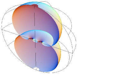
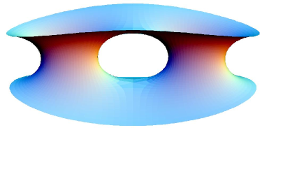
$k=2$
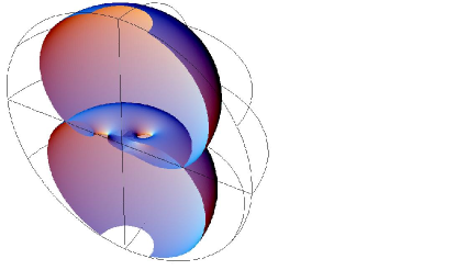
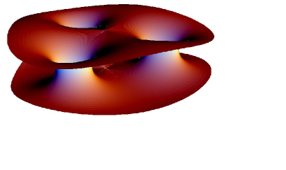
$k=3$
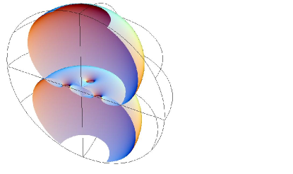
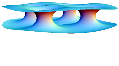
$k=8$

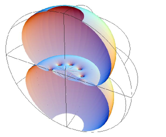
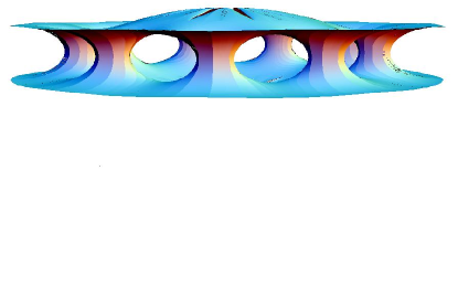
Figure 1. Half cut-away of higher genus catenoids in $H^{3}$ (in the Poincaré ball model), on the left, and central portions of those same surfaces on the right, for $k=1$, $k=2$, $k=3$ and $k=8$.

1. The Weierstrass data

Here we use a more general Weierstrass data than in [RS] and [F2], allowing the genus to be any positive number.

Take the compact Riemann surface

$$\overline{M}=\left\{(z,w)\in(\boldsymbol{C}\cup\{\infty\})^{2}\,\left|\,w^{k+1}=z\left(\frac{z-\lambda^{-1}}{\lambda-z}\right)^{k}\right.\right\}\;,$$

where $k$ is any positive integer and $\lambda$ is any real constant such that $\lambda>1$. This $\overline{M}$ has the structure of a Riemann surface, and $z$ provides a local complex coordinate for $\overline{M}$ at all but four points. At those four points $(0,0)$, $(\infty,\infty)$, $(\lambda,\infty)$ and $(\lambda^{-1},0)$, we can take a local coordinate $\zeta_{0}$, $\zeta_{\infty}$, $\zeta_{\lambda}$ and $\zeta_{\lambda^{-1}}$ satisfying $\zeta_{0}^{k+1}=z$, $\zeta_{\infty}^{-k-1}=z$, $\zeta_{\lambda}^{k+1}=z-\lambda$ and $\zeta_{\lambda^{-1}}^{k+1}=z-\lambda^{-1}$, respectively. By applying the Riemann-Hurwitz relation, we find that this Riemann surface has genus $k$. Then take

$$M=\overline{M}\setminus\{(0,0),(\infty,\infty)\}\;.$$

Here $(0,0)$ and $(\infty,\infty)$ will represent the two ends of the surfaces we will construct (surfaces having domain $M$). Let $\widetilde{M}$ be the universal cover of $M$.

We now take the Weierstrass data

(1.1) $$G=\lambda^{k/(k+1)}w\;,\;\;\;\Omega=c\cdot\frac{dz}{zw}\;.$$

Here $c$ is any nonzero real constant.

Remark 1.1.

Multiplying the hyperbolic Gauss map $G$ by a constant is equivalent to just a rigid motion of the surface, in both $H^{3}$ and $S^{3}_{1}$. So we could have chosen $G$ to be $G=w$ in Equation (1.1), as our goal is to construct surfaces in $H^{3}$ and $S^{3}_{1}$. However, when considering relations with minimal surfaces in $\boldsymbol{R}^{3}$ and maximal surface in $\boldsymbol{R}^{3}_{1}$, the choice of $G$ in (1.1) will prove to be useful, as we will see in Remark 2.4. So here we use the hyperbolic Gauss map $G$ as given in (1.1).

Note that $\deg(G)=k+1$. Now take a solution

$$F:\widetilde{M}\to\operatorname{SL}(2,\boldsymbol{C})$$

of

(1.2) $$dF\cdot F^{-1}=\begin{pmatrix}G&-G^{2}\\ 1&-G\end{pmatrix}\Omega\;.$$

Noting that, with $a^{*}=\bar{a}^{t}$,

$$H^{3}=\{aa^{*}\,|\,a\in\operatorname{SL}(2,\boldsymbol{C})\},\quad S^{3}_{1}=\{ae_{3}a^{*}\,|\,a\in\operatorname{SL}(2,\boldsymbol{C})\},\quad e_{3}=\begin{pmatrix}1&0\\ 0&-1\end{pmatrix},$$

define

(1.3) $$f_{H}:=FF^{*}:\widetilde{M}\to H^{3}\quad\text{and}\quad f_{S}:=Fe_{3}F^{*}:\widetilde{M}\to S^{3}_{1}.$$

Then $f_{H}$ (resp. $f_{S}$) gives a CMC $1$ immersion in $H^{3}$ (resp. a CMC $1$ face in $S^{3}_{1}$), since

(1.4) $$\left(1+|G|^{2}\right)^{2}\Omega\overline{\Omega}$$

gives a positive definite metric on $M$, see [UY3] and Theorem 1.9 of [F1]. Note that the Hopf differential of both $f_{H}$ and $f_{S}$ is written as

$$Q=\Omega dG=\frac{c\lambda^{k/(k+1)}}{k+1}\cdot\frac{z^{2}+\{(k-1)\lambda^{-1}-(k+1)\lambda\}z+1}{z^{2}(z-\lambda^{-1})(z-\lambda)}dz^{2}.$$

2. Symmetries of the surface

We define

$$w_{0}:=\lambda^{-k/(k+1)}\in\boldsymbol{R}\quad\text{and}\quad\Lambda:=e^{2\pi i/(k+1)}.$$

Then it is easy to see that

$$(1,\Lambda^{j}w_{0})\in M\quad\text{for any $j=0,1,\dots,k$}.$$

Consider the symmetries

$$\kappa_{1}(z,w)=\left(\bar{z},\bar{w}\right),\quad\kappa_{2}(z,w)=\left(\frac{1}{z},\frac{1}{\lambda^{2k/(k+1)}}\frac{1}{w}\right),\quad\kappa_{3}(z,w)=\left(\bar{z},\Lambda\bar{w}\right)$$

on $\overline{M}$. Then we have the following, which follows from a proof analogous to proofs found in [RS] and [F2]:

Lemma 2.1.

Let

$$F(z,w)=\begin{pmatrix}A&B\\ C&D\end{pmatrix}$$

be a solution of (1.2) with the initial condition $F(1,w_{0})=\operatorname{id}$. Then

(2.1) $$F(\kappa_{1}(z,w))=\begin{pmatrix}\bar{A}&\bar{B}\\ \bar{C}&\bar{D}\end{pmatrix},\quad F(\kappa_{2}(z,w))=\begin{pmatrix}D&C\\ B&A\end{pmatrix},\quad F(\kappa_{3}(z,w))=\begin{pmatrix}\bar{A}&\Lambda\bar{B}\\ \Lambda^{-1}\bar{C}&\bar{D}\end{pmatrix}.$$

Proof.

Note that we have the following relations under the symmetries $\kappa_{j}$:

$$G\circ\kappa_{1}=\bar{G}\;,\;\;\;G\circ\kappa_{2}=G^{-1}\;,\;\;\;G\circ\kappa_{3}=\Lambda\bar{G}\;,$$

$$\kappa_{1}^{*}\Omega=\bar{\Omega}\;,\;\;\;\kappa_{2}^{*}\Omega=-\lambda^{2k/(k+1)}w^{2}\Omega\;,\;\;\;\kappa_{3}^{*}\Omega=\Lambda^{-1}\bar{\Omega}\;.$$

It follows that

$$\kappa_{1}^{*}\begin{pmatrix}G&-G^{2}\\ 1&-G\end{pmatrix}\Omega =\overline{\begin{pmatrix}G&-G^{2}\\ 1&-G\end{pmatrix}\Omega}\;,$$

$$\kappa_{2}^{*}\begin{pmatrix}G&-G^{2}\\ 1&-G\end{pmatrix}\Omega =\begin{pmatrix}0&i\\ i&0\end{pmatrix}^{-1}\begin{pmatrix}G&-G^{2}\\ 1&-G\end{pmatrix}\Omega\begin{pmatrix}0&i\\ i&0\end{pmatrix}\;,$$

$$\kappa_{3}^{*}\begin{pmatrix}G&-G^{2}\\ 1&-G\end{pmatrix}\Omega =\begin{pmatrix}\sqrt{\Lambda}&0\\ 0&1/\sqrt{\Lambda}\end{pmatrix}\overline{\begin{pmatrix}G&-G^{2}\\ 1&-G\end{pmatrix}\Omega}\begin{pmatrix}1/\sqrt{\Lambda}&0\\ 0&\sqrt{\Lambda}\end{pmatrix}\;.$$

Because the initial condition $F(1,w_{0})=\operatorname{id}$ satisfies

$$\overline{F(1,w_{0})}=F(1,w_{0})\;,\qquad\begin{pmatrix}0&i\\ i&0\end{pmatrix}^{-1}\!\!\!F(1,w_{0})\begin{pmatrix}0&i\\ i&0\end{pmatrix}=F(1,w_{0})\;,$$

$$\begin{pmatrix}\sqrt{\Lambda}&0\\ 0&1/\sqrt{\Lambda}\end{pmatrix}\overline{F(1,w_{0})}\begin{pmatrix}1/\sqrt{\Lambda}&0\\ 0&\sqrt{\Lambda}\end{pmatrix}=F(1,w_{0})\;,$$

the lemma follows. ∎

We now consider two loops in $M$ (see Figure 2):

Figure 2. Projection to the $z$-plane of the loops $\gamma_{1}$ and $\gamma_{2}$. (Note that $z=1$ is not a branch point of $M$, and $\gamma_{1}$ starts at one lift of $z=1$, and then passes through another lift of $z=1$, and then returns to the first lift of $z=1$.)

• The loop $\gamma_{1}:[0,1]\to M$ starts at $\gamma_{1}(0)=(1,w_{0})\in M$. Its first portion has $z$ coordinate in $\{\operatorname{Im}(z)<0\}$ and ends at a point $(z,w)$ where $z\in\boldsymbol{R}$ and $0<z<\lambda^{-1}$. Its second portion starts at $(z,w)$ and ends at $(1,\Lambda w_{0})$ and has $z$ coordinate in $\{\operatorname{Im}(z)>0\}$. Its third portion starts at $(1,\Lambda w_{0})$ and ends at $(1/z,\Lambda/(\lambda^{2k/(k+1)}w))$ and has $z$ coordinate in $\{\operatorname{Im}(z)>0\}$. Its fourth and last portion starts at $(1/z,\Lambda/(\lambda^{2k/(k+1)}w))$ and returns to the base point $\gamma_{1}(1)=(1,w_{0})$ and has $z$ coordinate in $\{\operatorname{Im}(z)<0\}$.

• The loop $\gamma_{2}:[0,1]\to M$ starts at $\gamma_{2}(0)=(1,w_{0})$. Its first portion has $z$ coordinate in $\{\operatorname{Im}(z)<0\}$ and ends at a point $(z,w)$ where $z\in\boldsymbol{R}$ and $z<0$. Its second and last portion starts at $(z,w)$ and returns to $\gamma_{2}(1)=(1,w_{0})$ and has $z$ coordinate in $\{\operatorname{Im}(z)>0\}$.

We will also consider the following two paths (not loops) in $M$ (see Figure 3):

Figure 3. Projection to the $z$-plane of the curves $c_{1}$ and $c_{2}$.

• Let $c_{1}:[0,1]\to M$ be a curve starting at $c_{1}(0)=(1,w_{0})$ whose projection to the $z$-plane is an embedded curve in $\{\operatorname{Im}(z)<0\}$, and whose endpoint $c_{1}(1)$ has a $z$ coordinate so that $z\in\boldsymbol{R}$ and $0<z<\lambda^{-1}$.

• Let $c_{2}(t):[0,1]\to M$ be a curve starting at $c_{2}(0)=(1,w_{0})$ whose projection to the $z$-plane is an embedded curve in $\{\operatorname{Im}(z)<0\}$, and whose endpoint $c_{2}(1)$ has a $z$ coordinate so that $z\in\boldsymbol{R}$ and $z<0$.

With $F(1,w_{0})=\operatorname{id}$, we solve Equation (1.2) along these two paths to find

$$F(c_{1}(1))=\begin{pmatrix}A_{1}&B_{1}\\ C_{1}&D_{1}\end{pmatrix},\quad\text{and}\quad F(c_{2}(1))=\begin{pmatrix}A_{2}&B_{2}\\ C_{2}&D_{2}\end{pmatrix}.$$

Let $\tau_{j}$ be the deck transformation of $\widetilde{M}$ associated to the homotopy class of $\gamma_{j}$ ($j=1,2$).

Lemma 2.2.

We have that $F\circ\tau_{1}=F\Phi_{1}$ and $F\circ\tau_{2}=F\Phi_{2}$, where

$$\Phi_{1} :=\begin{pmatrix}\bar{A}_{1}&-\bar{C}_{1}\\ -\bar{B}_{1}&\bar{D}_{1}\end{pmatrix}\begin{pmatrix}D_{1}&\Lambda C_{1}\\ \Lambda^{-1}B_{1}&A_{1}\end{pmatrix}\begin{pmatrix}\bar{D}_{1}&-\Lambda\bar{B}_{1}\\ -\Lambda^{-1}\bar{C}_{1}&\bar{A}_{1}\end{pmatrix}\begin{pmatrix}A_{1}&B_{1}\\ C_{1}&D_{1}\end{pmatrix}\;,$$

$$\Phi_{2} :=\begin{pmatrix}\bar{D}_{2}&-\bar{B}_{2}\\ -\bar{C}_{2}&\bar{A}_{2}\end{pmatrix}\begin{pmatrix}A_{2}&B_{2}\\ C_{2}&D_{2}\end{pmatrix}\;.$$

Proof.

The loop $\gamma_{1}$ has four portions, as described above. The first portion is represented by the curve $c_{1}$. The second portion is represented by $\kappa_{3}\circ c_{1}^{-1}$. Using the facts that the third portion starts at the point $(1,\Lambda w_{0})$ and that $\kappa_{2}\circ\kappa_{1}\circ\kappa_{3}(1,w_{0})=(1,\Lambda w_{0})$, we have that the third portion is represented by $\kappa_{2}\circ\kappa_{1}\circ\kappa_{3}\circ c_{1}$. The final fourth portion is represented by $\kappa_{1}\circ\kappa_{2}\circ c_{1}^{-1}$, which follows from noting that $\kappa_{1}(1,w_{0})=(1,w_{0})$, $\kappa_{2}(1,w_{0})=(1,w_{0})$ and $\kappa_{3}(1,w_{0})=(1,\Lambda w_{0})$. (In particular, we see that $(1,w_{0})$ is in the fixed point set of $\kappa_{1}$ and $\kappa_{2}$ but not in that of $\kappa_{3}$.)

Thus we have that

$$\gamma_{1}=(\kappa_{1}\circ\kappa_{2}\circ c_{1}^{-1})\circ(\kappa_{2}\circ\kappa_{1}\circ\kappa_{3}\circ c_{1})\circ(\kappa_{3}\circ c_{1}^{-1})\circ c_{1}\;.$$

Similarly, we can see that

$$\gamma_{2}=(\kappa_{1}\circ c_{2}^{-1})\circ c_{2}\;.$$

We can then apply Lemma 2.1 to get the result. ∎

Using the Bryant type representation (1.3) to make CMC $1$ surfaces in $H^{3}$ and $S_{1}^{3}$, the conditions for the resulting surfaces to be well defined on $M$ are that $\Phi_{1}$ and $\Phi_{2}$ are in $\operatorname{SU}(2)$ and $\operatorname{SU}(1,1)$, respectively, and by symmetry, only the homotopy classes coming from $\gamma_{1}$ and $\gamma_{2}$ need be considered. However, the initial condition $F(1,w_{0})=\operatorname{id}$ will not cause $\Phi_{1}$ and $\Phi_{2}$ to lie in $\operatorname{SU}(2)$ or $\operatorname{SU}(1,1)$. To remedy this, we will change the initial condition for the solution $F$ so that it has initial condition

$$F(1,w_{0})=\begin{pmatrix}\alpha&\beta\\ \beta&\alpha\end{pmatrix}\in\operatorname{SL}(2,\boldsymbol{R})$$

in the case the ambient space is $H^{3}$ (that is, the $\operatorname{SU}(2)$ case), and

$$F(1,w_{0})=\begin{pmatrix}\alpha&\beta\\ \alpha&-\beta\end{pmatrix}\in\operatorname{SL}(2,\boldsymbol{R})$$

in the case the ambient space is $S^{3}_{1}$ (that is, the $\operatorname{SU}(1,1)$ case).

Note that with these changes of initial condition of $F$, we still have enough symmetry to conclude that the resulting surfaces are well defined on $M$ just by looking only at the two homotopy classes represented by $\gamma_{1}$ and $\gamma_{2}$. This is because the homotopy group of $M$ is generated by $[\gamma_{1}]$ and $[\gamma_{2}]$. The monodromies associated to those two homotopy classes are now, for $j=1,2$,

$$\begin{pmatrix}\alpha&\beta\\ \beta&\alpha\end{pmatrix}^{-1}\Phi_{j}\begin{pmatrix}\alpha&\beta\\ \beta&\alpha\end{pmatrix}$$

in the $\operatorname{SU}(2)$ case, and

$$\begin{pmatrix}\alpha&\beta\\ \alpha&-\beta\end{pmatrix}^{-1}\Phi_{j}\begin{pmatrix}\alpha&\beta\\ \alpha&-\beta\end{pmatrix}$$

in the $\operatorname{SU}(1,1)$ case.

The closing conditions, that is, the conditions that the surfaces are well defined on $M$ itself, are now that the above pairs of matrices lie in $\operatorname{SU}(2)$ in the first case, and in $\operatorname{SU}(1,1)$ in the second case. Noting that $\Phi_{1}$ and $\Phi_{2}$ take the forms

$$\Phi_{1}=\begin{pmatrix}r_{1}&p\\ -\bar{p}&r_{2}\end{pmatrix}\;,\quad\Phi_{2}=\begin{pmatrix}q&ir_{3}\\ ir_{4}&\bar{q}\end{pmatrix}$$

for complex numbers $p$, $q$ and real numbers $r_{1}$, $r_{2}$, $r_{3}$, $r_{4}$, a direct computation gives that the closing conditions are

$$\frac{2\operatorname{Re}(p)}{r_{2}-r_{1}}=\frac{2\operatorname{Im}(q)}{r_{4}-r_{3}}=\frac{\alpha^{2}+\beta^{2}}{2\alpha\beta}=\frac{1+2\beta^{2}}{2\beta\sqrt{1+\beta^{2}}}\in(-\infty,-1)\cup(1,\infty)$$

in the $\operatorname{SU}(2)$ case, and

$$\frac{2\operatorname{Re}(p)}{r_{2}-r_{1}}=\frac{2\operatorname{Im}(q)}{r_{4}-r_{3}}=\frac{\alpha^{2}-\beta^{2}}{\alpha^{2}+\beta^{2}}=\frac{1-4\beta^{4}}{1+4\beta^{4}}\in(-1,1)$$

in the $\operatorname{SU}(1,1)$ case. So we have now proven the following lemma:

Lemma 2.3.

The single closing condition for one of the surfaces in (1.3) is that

(2.2) $$h_{1}(c,\lambda)=h_{2}(c,\lambda)\in\boldsymbol{R}\setminus\{\pm 1\},$$

where

$$h_{1}(c,\lambda)=\frac{2\operatorname{Re}(p)}{r_{2}-r_{1}}\quad\text{and}\quad h_{2}(c,\lambda)=\frac{2\operatorname{Im}(q)}{r_{4}-r_{3}}$$

holds, and then the appropriate $\alpha$ and $\beta$ can be found. Whether one obtains a surface in $H^{3}$ or $S_{1}^{3}$ is determined by whether the absolute value of $h_{1}(c,\lambda)=h_{2}(c,\lambda)$ is greater than or less than $1$.

Remark 2.4.

If we consider the minimal surface

$$\operatorname{Re}\int\left(1-G^{2},\,i(1+G^{2}),\,2G\right)\Omega\in\boldsymbol{R}^{3}$$

with the Weierstrass data (1.1), one can check that the period is solved for the loop $\gamma_{1}$ (regardless of the choice of $\lambda$, and we chose $G$ as we did in (1.1) in order to make this true, see Remark 1.1), but is never solved for the loop $\gamma_{2}$ (for any choice of $\lambda$). On the other hand, if we consider the maximal surface

$$\operatorname{Re}\int\left(1+G^{2},\,i(1-G^{2}),\,2G\right)\Omega\in\boldsymbol{R}^{3}_{1}$$

with the Weierstrass data (1.1), the period is solved for $\gamma_{2}$, but never for $\gamma_{1}$. See Figure 4.

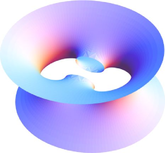
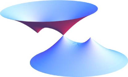
Figure 4. A minimal surface in $\boldsymbol{R}^{3}$ (left) and a maximal surface in $\boldsymbol{R}_{1}^{3}$ (right), constructed as in Remark 2.4, with $k=1$ and $\lambda=2$, in each case showing closing with respect to one loop $\gamma_{j}$ but not with respect to the other.

3. Numerical experiments and the main result

Fix $\lambda=2$. Here we provide constants $c\in\boldsymbol{R}\setminus\{0\}$ so that $h_{1}(c,2)=h_{2}(c,2)$ for the genus $k=1,\dots,20$ cases. It is a simple application of the intermediate value theorem to show $h_{1}(c,2)=h_{2}(c,2)$, and the functions $h_{j}(c,2)$ are stable with respect to numerics if the paths $c_{i}(t)$ are chosen well – so the numerics are not delicate, and are expected to give reliable results. Furthermore, once we have existence of a surface for one value of $\lambda=\lambda_{0}$, we then have existence for all $\lambda$ sufficiently close to $\lambda_{0}$, so we can conclude existence of a $1$-parameter family of such surfaces.

$k$	$c\in\boldsymbol{R}\setminus\{0\}$ so that $h_{1}(c,2)=\phantom{=}$ $\phantom{==}h_{2}(c,2)$	$h_{j}(c,2)$	$c\in\boldsymbol{R}\setminus\{0\}$ so that $h_{1}(c,2)=\phantom{=}$ $\phantom{==}h_{2}(c,2)$	$h_{j}(c,2)$	$c\in\boldsymbol{R}\setminus\{0\}$ so that $h_{1}(c,2)=\phantom{=}$ $\phantom{==}h_{2}(c,2)$	$h_{j}(c,2)$
1	$-$0.04675520	$-$6.91432	$-$0.557726	$-$0.130869	0.704094	$-$0.2212280
2	$-$0.04039010	$-$4.12613	$-$0.505010	$-$0.218257	0.548964	$-$0.0345248
3	$-$0.03345460	$-$3.32773	$-$0.483326	$-$0.254392	0.482090	$-$0.0678105
4	$-$0.02819310	$-$2.95960	$-$0.471988	$-$0.273656	0.444727	$-$0.1324290
5	$-$0.02425740	$-$2.74968	$-$0.465097	$-$0.285460	0.420845	$-$0.1769310
6	$-$0.02124670	$-$2.61454	$-$0.460530	$-$0.293371	0.404255	$-$0.2094430
7	$-$0.01888360	$-$2.52044	$-$0.457291	$-$0.299018	0.392055	$-$0.2342330
8	$-$0.01698500	$-$2.45121	$-$0.454881	$-$0.303237	0.382705	$-$0.2537600
9	$-$0.01542870	$-$2.39818	$-$0.453020	$-$0.306504	0.375309	$-$0.2695380
10	$-$0.01413100	$-$2.35627	$-$0.451543	$-$0.309105	0.369312	$-$0.2825530
11	$-$0.01303300	$-$2.32232	$-$0.450342	$-$0.311222	0.364352	$-$0.2934720
12	$-$0.01209240	$-$2.29427	$-$0.449348	$-$0.312979	0.360180	$-$0.3027640
13	$-$0.01127780	$-$2.27070	$-$0.448511	$-$0.314459	0.356623	$-$0.3107660
14	$-$0.01056550	$-$2.25062	$-$0.447797	$-$0.315722	0.353553	$-$0.3177300
15	$-$0.00993749	$-$2.23331	$-$0.447182	$-$0.316813	0.350878	$-$0.3238460
16	$-$0.00937975	$-$2.21824	$-$0.446645	$-$0.317764	0.348525	$-$0.3292600
17	$-$0.00888113	$-$2.20499	$-$0.446173	$-$0.318600	0.346439	$-$0.3340860
18	$-$0.00843272	$-$2.19326	$-$0.445756	$-$0.319341	0.344578	$-$0.3384150
19	$-$0.00802733	$-$2.18280	$-$0.445383	$-$0.320003	0.342907	$-$0.3423190
20	$-$0.00765905	$-$2.17341	$-$0.445049	$-$0.320596	0.341398	$-$0.3458590

Table 1. Numerical results with $\lambda=2$. The first column gives CMC $1$ surfaces in $H^{3}$. The second column gives CMC $1$ faces in $S^{3}_{1}$ with elliptic ends. The third column gives CMC $1$ faces in $S^{3}_{1}$ with hyperbolic ends.

The data in Table 1 (see also Figure 5) then imply the numerical result stated in the introduction, except that we still need to analyze the behavior of the ends. Because $\text{deg}(G)=k+1$, equality in the Osserman inequality is satisfied, for both the $H^{3}$ and $S_{1}^{3}$ cases. From this, it follows that the ends are complete and embedded in the $H^{3}$ case, and also in the $S_{1}^{3}$ case when the ends are elliptic (see [RS] and [F2], for example). When the ends are hyperbolic in $S_{1}^{3}$, they are neither complete nor embedded, but are weakly complete, because the metric (1.4) is complete, see [FRUYY]. However, we have yet to show when the ends are elliptic or hyperbolic in the $S_{1}^{3}$ case. This final step is taken care of by the next lemma, which is similar to arguments found in the appendix of [F2], but here we are allowing for the case of general genus $k$.

Figure 5. Graphs of the functions $h_{1}(c,2)$ (thin curve) and $h_{2}(c,2)$ (thick curve) in six cases: $k=1$ in $H^{3}$ (upper left), $k=1$ in $S_{1}^{3}$ with elliptic ends (upper middle), $k=1$ in $S_{1}^{3}$ with hyperbolic ends (upper right), $k=2$ in $H^{3}$ (lower left), $k=2$ in $S_{1}^{3}$ with elliptic ends (lower middle), $k=2$ in $S_{1}^{3}$ with hyperbolic ends (lower right).

Lemma 3.1.

The ends of the CMC $1$ faces in $S_{1}^{3}$ in the middle column $($resp. right hand column$)$ of Table 1 have elliptic $($resp. hyperbolic$)$ ends.

Proof.

Let

$$F=\begin{pmatrix}A&B\\ C&D\end{pmatrix}$$

be a solution to (1.2). Note that, in order to determine the type of monodromy about an end, we only need to know the eigenvalues of the monodromy (provided those eigenvalues are not $\pm 1$), and this is independent of the choice of $F$. So we may choose any solution to (1.2). We then have

$$X_{zz}+\left(\frac{1}{z}-\frac{w_{z}}{w}\right)X_{z}+\lambda^{k/(k+1)}\frac{cw_{z}}{zw}X=0\;,\;\;\;X=A,B\;,$$

and

$$Y_{zz}+\left(\frac{1}{z}+\frac{w_{z}}{w}\right)Y_{z}+\lambda^{k/(k+1)}\frac{cw_{z}}{zw}Y=0\;,\;\;\;Y=C,D\;.$$

Because of the symmetry $\kappa_{2}(z,w)$, it suffices to determine the type of just one end, and then the other end will automatically have the same type. So let us choose the end $(z,w)=(0,0)$. At this end, $w$ is a local coordinate for the Riemann surface $\overline{M}$. In terms of $w$, and considering $z$ as a function of $w$, the equations above become

$$X_{ww}+o(1)\frac{X_{w}}{w}+\lambda^{k/(k+1)}c(k+1)\left(1+o(1)\right)\frac{X}{w^{2}}=0\;,\;\;\;X=A,B\;,$$

and

$$Y_{ww}+2\left(1+o(1)\right)\frac{Y_{w}}{w}+\lambda^{k/(k+1)}c(k+1)\left(1+o(1)\right)\frac{Y}{w^{2}}=0\;,\;\;\;Y=C,D\;,$$

where $o(1)$ denotes the Landau symbol, that is, $o(1)$ is a holomorphic function $\varphi(w)$ around $(z,w)=(0,0)$ so that $\varphi(0)=0$. It follows that the difference of the solutions of the indicial equation corresponding to the first of these two equations is

$$\sqrt{1-4c(k+1)\lambda^{k/(k+1)}}\;.$$

Likewise, the difference of solutions of the indicial equation for the second equation above takes the same value. It follows (see the appendix of [F2] for further details) that the end is elliptic (resp. hyperbolic) if

$$1-4c(k+1)\lambda^{k/(k+1)}$$

is positive (resp. negative) which is indeed the case for the data given in the middle column (resp. right hand column) of Table 1. ∎

References

- [AA] R. Aiyama and K. Akutagawa, Kenmotsu-Bryant type representation formulas for constant mean curvature surfaces in and , Ann. Global Anal. Geom. 17 (1998), 49-75.
- [B] R. Bryant, Surfaces of mean curvature one in hyperbolic space, Astérisque 154–155 (1987), 321-347.
- [F1] S. Fujimori, Spacelike CMC surfaces with elliptic ends in de Sitter -space, Hokkaido J. Math. 35 (2006), 289–320.
- [F2] by same author, Spacelike mean curvature surfaces of genus with two ends in de Sitter -space, Kyushu J. Math. 61 (2007), 1–20.
- [FRUYY] S. Fujimori, W. Rossman, M. Umehara, K. Yamada and S-D. Yang, Spacelike mean curvature one surfaces in de Sitter -space, Comm. Anal. Geom. 17 (2009), 383–427.
- [FS] S. Fujimori and T. Shoda, Minimal surfaces with two ends which have the least total absolute curvature, preprint.
- [KY] Y. W. Kim and S-D. Yang, A family of maximal surfaces in Lorentz-Minkowski three-space, Proc. Amer. Math. Soc. 134 (2006), 3379–3390.
- [K] O. Kobayashi, Maximal surfaces in the -dimensional Minkowski space , Tokyo J. Math. 6 (1983), 297-309.
- [LR] G. Levitt and H. Rosenberg, Symmetry of constant mean curvature hypersurfaces in hyperbolic space, Duke Math. J. 52 (1985), 53–59.
- [RS] W. Rossman and K. Sato, Constant mean curvature surfaces in hyperbolic -space with two ends, J. Exp. Math. 7 (1998), 101–119.
- [RUY1] W. Rossman, M. Umehara and K. Yamada, Irreducible CMC- surfaces in with positive genus, Tohoku Math. J. 49 (1997), 449–484.
- [RUY2] by same author, Mean curvature surfaces in hyperbolic -space with low total curvature, Tohoku Math. J. 55 (2003), 375–395.
- [S] R. Schoen, Uniqueness, symmetry, and embeddedness of minimal surfaces, J. Diff. Geom. 18 (1983), 791–809.
- [UY1] M. Umehara and K. Yamada, Complete Surfaces of Constant Mean Curvature One in the Hyperbolic 3-Space, Ann. of Math., 137 (1993), 611–638.
- [UY2] by same author, Surfaces of Constant Mean Curvature in with prescribed hyperbolic Gauss map, Math. Ann. 304 (1996), 203–224.
- [UY3] by same author, A duality on CMC- surfaces in hyperbolic space, and a hyperbolic analogue of the Osserman inequality Tsukuba J. Math. 21 (1997), 229–237.
- [UY4] by same author, Maximal surfaces with singularities in Minkowski space, Hokkaido Math. J. 35 (2006), 13–40.