Homological characterizations of spiral defect chaos in Rayleigh-Bénard convection

Abstract

We use a quantitative topological characterization of complex dynamics to measure geometric structures. This approach is used to analyze the weakly turbulent state of spiral defect chaos in experiments on Rayleigh-Bénard convection. Different attractors of spiral defect chaos are distinguished by their homology. The technique reveals pattern asymmetries that are not revealed using statistical measures. In addition we observe global stochastic ergodicity for system parameter values where locally chaotic dynamics has been observed previously.

Characterization of geometric structures (patterns) in physical systems can give insight into underlying dynamics. For simple cases, pattern characterization is easily done with a few numbers (e.g. the lattice constants describing problems with crystalline symmetries). However encoding patterns becomes more difficult as patterns become more complex. Statistical approaches can be used to describe complex patterns in dynamically evolving systems Morris et al. (1996); Ecke et al. (1995); however, a general methodology for extracting geometric signatures from complex patterns has been lacking.

We describe an approach that uses algebraic topology to extract consistent and robust geometric properties from experimental observations of spatiotemporal complexity. We employ homology theory since it is the most computable algebraic topological invariant (i.e., remains constant under deformations and is independent of any particular metric) that still provides detailed geometric information. Hydrodynamic systems readily produce complex spatiotemporal patterns Manneville (1990), which are ideal for testing these techniques. We use homology to obtain a limited set of numbers (called Betti numbers defined below) that characterize dynamically relevant features in a weakly turbulent state of Rayleigh-Bénard convection (RBC) known as spiral defect chaos (SDC) Morris et al. (1993) (see Fig. 1). In particular, we find that: (a) the geometric structures of asymptotic states of SDC are readily distinguishable as a function of a control parameter; (b) the entropy of the SDC attractors quantifies the evolution of the system through different geometric configurations; (c) the asymptotic global geometric configurations evolve stochastically as opposed to chaotically as identified previously Egolf et al. (1998, 2000); (d) symmetry breaking in the flow patterns is readily detectable in cases where simple statistical measures (e.g., measurements of mean pattern volumes) are insensitive to pattern asymmetries; and (e) the boundary and bulk patterns can be distinguished.

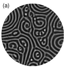
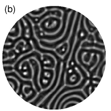
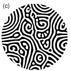
Figure 1: Shadowgraph images of spiral defect chaos convection patterns at reduced Rayleigh numbers $\epsilon\approx 1.0$ (a) and $\epsilon\approx 2.0$ (b) are converted to binary valued images [(c) and (d), respectively] by thresholding the data at the median value of intensity. In (c) and (d), the black regions correspond to hot upflow, and the white regions to cold downflow.

We measure convective flow in a 0.069 cm deep horizontal layer of CO₂ gas at a pressure of 3.2 MPa bounded above by a 5 cm thick sapphire window and below by 1 cm thick gold plated aluminum mirror. The lateral walls are circular, formed out of an annular stack of filter paper sheets 3.8 cm in diameter. An electrical resistive heater is used to heat the bottom mirror, and the top window is cooled by circulating chilled water at 21.2 ^oC. When the vertical temperature difference, $T$, across the gas exceeds a critical temperature difference, $T_{c}\approx 4$ ^oC, the onset of fluid motion occurs. The flow organizes into a pattern of convective rolls where hot regions of the gas move upward and cold regions flow downward. The convection rolls become spatially disordered and exhibit complex time dependence when the system control parameter $\epsilon=(T-T_{c})/T_{c}$ (the reduced Rayleigh number) is sufficiently large. For the present study, the patterns are observed for the order of $10^{4}\tau_{\nu}$ ($\tau_{\nu}\approx 2.1$ seconds is the vertical thermal diffusion time) at $\epsilon\approx 1.0$ and $\epsilon\approx 2.0$.

Shadowgraph visualization of the convecting flow yields intensity images, which are used to compute the topology of the rolls in SDC (Fig. 1). The shadowgraph technique is sensitive to the refractive index variations in the gas, which represents the temperature profile of the flow Settles (2001). The state of the flow is sampled at 11 Hz by capturing raw intensity images [Fig. 1 (a) & (b)] using a 12-bit digital camera; a background image of the fluid below the onset of convection is then subtracted to remove optical nonuniformities (e.g., optical imperfections in the bottom plate). Digital Fourier filtering is then applied to remove high wavenumber components due to camera spatial noise. The data is then converted to binary values by thresholding at the median value of intensity. The resulting images [Fig. 1 (c) & (d)], where black represents hot upflow and white represents cold downflow, are used as input to computation of homology. In what follows, $X(n,\epsilon)$ represents the $n^{th}$ binary image in a time series at the reduced Rayleigh number $\epsilon$. Moreover, $X^{hot}(n,\epsilon)$ and $X^{cold}(n,\epsilon)$ denote the hot flow and cold flow regions, respectively, of $X(n,\epsilon)$. It is worth noting that the number of pixels in $X^{hot}(n,\epsilon)$ is equal to the number of pixels in $X^{cold}(n,\epsilon)$, i.e., hot and cold regions occupy the same area in the pattern.

Homology theory provides a rigorous, systematic, and dimension independent method for characterizing geometric structures in $X(n,\epsilon)$ using a few numbers. More specifically, the homology of a structure $X$ in two dimensions (e.g., $X^{hot}(n,\epsilon)$ or $X^{cold}(n,\epsilon)$) is characterized by two nonnegative integers $\beta_{i}$, $i=0,1$ called Betti numbers, where $\beta_{0}$ counts the number of connected components (pieces) of $X$, and $\beta_{1}$ is equal the number of holes in $X$. A concrete illustration of this classification applied to convection patterns is given in Fig. 2. (For a more detailed discussion see Gameiro et al. (2004); Kaczynski et al. (2004).) The computations were done using the package CHomP Kalies and Pilarczyk (2003); Kaczynski et al. (2004). Typically it takes about 10 seconds to reduce each shadowgraph image (of size 515 x 650 pixels) to binary form and to compute its homology.

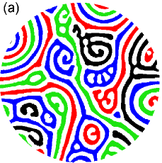
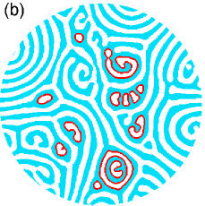
Figure 2: (Color online) Betti numbers for the $X^{hot}$ region shown in Fig. 1 (c). Image (a) shows the $\beta_{0}^{hot}=34$ distinct components, with neighboring components distinguished by different colors. Image (b) indicates the boundaries of the $\beta_{1}^{hot}=13$ holes. The only components, out of the $\beta_{0}^{cold}=38$, of $X^{cold}$ (white region) that do not touch the boundary are the ones enclosed by the $\beta_{1}^{hot}=13$ loops in $X^{hot}$. So the number of components of $X^{cold}$ touching the boundary is $\beta_{0}^{cold}-\beta_{1}^{hot}=25$.

Parameter Distinction.— The sequence of Betti numbers can be used to clearly distinguish different complex states of SDC (Fig. 3). For the Rayleigh numbers $\epsilon\approx 1.0$ and $\epsilon\approx 2.0$ we calculated sequences of Betti numbers $\beta^{hot}_{i}(n,\epsilon)$ and $\beta^{cold}_{i}(n,\epsilon)$, $n=0,\ldots,50,000$. Figure  3 shows that the time average of the Betti numbers are different at different $\epsilon$.

The difference in the mean values of the Betti numbers (Fig. 3) reflects the instability mechanisms operating during the evolution of the complex spatiotemporal pattern in SDC. The dynamically significant events for the evolution occur in regions of local compression or dilatation of the roll structure. The compression leads to the merging of neighboring rolls while the dilatation results in the formation of a new roll in the pattern. Such local events change the topology of the pattern. For instance, the merging of two rolls reduces the number of distinct rolls reducing $\beta_{0}$ by one. A pattern increasingly dominated by such instabilities would hence show an overall reduction in $\beta_{0}$ as different components link together locally at distinct locations. As the number of distinct rolls reduces, such linkages are often self-intersections of a roll. This manifests as an increase in the number of loops ($\beta_{1}$) in the pattern. The mechanisms characterizing the secondary instabilities for ideal straight rolls Busse (1967) have a similar structure and are known as the skew-varicose (compression) and the cross-roll (dilatation) instabilities. In spiral defect chaos such events are seen to be operational in regions localized by the curvature of the rolls.

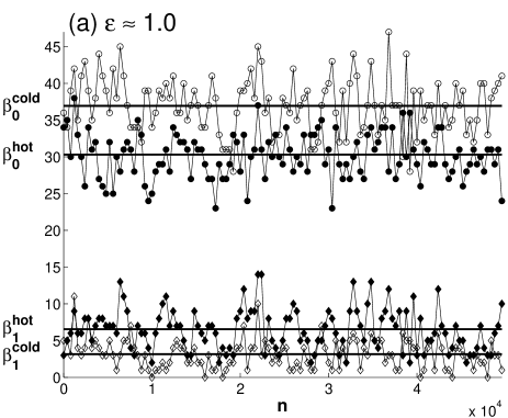
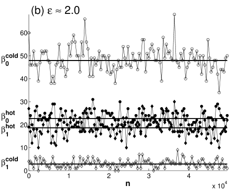
Figure 3: Time series of Betti numbers showing every 400th data point of the time evolution of the number of distinct components and holes in the regions $X^{hot}$ (closed, black symbols) and $X^{cold}$ (open, white symbols). The complete time series plots are qualitatively similar to the ones shown, the data is partially sampled only for better visualization. Circles correspond to $\beta_{0}$ and diamonds to $\beta_{1}$. The horizontal lines indicate the mean values $\bar{\beta}_{i}(\epsilon)$ for the corresponding time series. Image (a) is for $\epsilon\approx 1.0$ and (b) for $\epsilon\approx 2.0$.

Entropy.— At different parameter values, the state of SDC converges to different attractors. The signature of convergence to the attractor is the evolution of the system in a bounded neighborhood in the space spanned by the Betti numbers. The set of Betti numbers describes the different patterns of rolls attained by the system. A complete description of the homological configuration of the state is determined by the set of Betti numbers describing the hot and the cold regions.

We calculate the probability of being in a particular configuration from a long time series of Betti numbers for the evolution of the state while on the attractor. The probability distribution enables the computation of an entropy to distinguish between different SDC attractors. The entropy is defined as

$$S(\epsilon)=-\sum_{i}p_{i}log(p_{i}),$$

where the index $i$ span the different states attained by the system as characterized by the Betti numbers. We denote by $p_{i}$ the probability of being in a particular state described by $\beta^{hot}_{0}$, $\beta^{hot}_{1}$,$\beta^{cold}_{0}$ and $\beta^{cold}_{1}$. The probability is obtained by trivially counting the number of distinct configurations attained over a large (ergodic) period of time and normalizing by the total number of possible configurations. While the entropy is computed over the states attained by the system in a finite amount of time, its value is seen to asymptote to a constant for long time series as the probability distribution of the Betti numbers at the attractor converges. In states where the components do not interact, the entropy reduces as a result of no fluctuations in the Betti numbers associated with defect formation. The entropy increases for attractors that show evolving topologies mediated through defects. We find that the entropy of the system increases from 8.927 to 9.631 as $\epsilon$ is increased from $\epsilon\approx 1.0$ to $\epsilon\approx 2.0$.

Stochastic Evolution.— The evolution of complex geometries may be distinguished as being chaotic or stochastic from the time series of Betti numbers. The sequence of Betti numbers has been used to uncover global chaotic evolution through the computation of the largest Lyapunov exponent in numerical simulations of reaction-diffusion systems previously Gameiro et al. (2004). In our experiments on SDC we have been unsuccessful in extracting Lyapunov exponents using similar techniques. In the case of SDC a mechanism describing locally chaotic islands driving the complex dynamics has been proposed Egolf et al. (1998, 2000). It is likely that the spatiotemporally localized nature of such instabilities in SDC decorrelates at a scale that is not effectively captured by the time series of Betti numbers; a succession of these local events interspersed across the system may cause effectively stochastic evolution for the global geometric structure attained at the attractor. To first order we find it likely that the dynamics of fluctuations in the Betti numbers may be primarily stochastic in nature, as it is also suggested by the auto-correlation of the time series (Fig. 4).

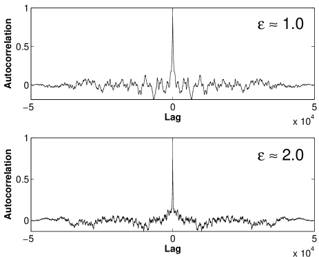
Figure 4: The autocorrelation for the time series of the number of holes ($\beta_{1}$) in a state of SDC. The spiked nature of the function suggests that the fluctuations are primarily stochastic with little correlation. The autocorrelation for $\beta_{0}$ has a similar spiked shape.

Symmetry Breaking.— The homology of the states exhibited by SDC uncovers a break in the symmetry between upflows and downflows. For an ideal Rayleigh-Bénard problem, as described by the Boussinesq equations Chandrasekhar (1961), the inversion of the sign of the velocity (and time) is also a solution to the evolution equations. This symmetry of the flow (the Boussinesq symmetry) in an ideal Rayleigh-Bénard problem suggests that the statistical properties of the patterns would be the same for $X^{hot}$ and $X^{cold}$; in particular we should obtain $\bar{\beta}_{i}^{hot}(\epsilon)=\bar{\beta}_{i}^{cold}(\epsilon)$ for $i=0,1$. As Fig. 3 indicates, in our experiments we found that that the mean values of the Betti numbers clearly distinguish between fluid regions comprised of hot and cold flows. Furthermore, this asymmetry is enhanced with an increase in the Rayleigh number. We suspect that the pattern homology serves as a sensitive detector of non-Boussinesq effects that are present due to the variation in physical properties of the fluid between the hot bottom layer and the cool top layer. The strength of non-Boussinesq effects in experiments can be estimated by a dimensionless parameter $Q$ Busse (1967); Cross and Hohenberg (1993) computed perturbatively at the primary instability for convection. In our experiments with CO₂, we find this parameter to be equal 0.54 near the onset of convection — thus indicating strong, $O(1)$, non-Boussinesq effects. A similar computation at $\epsilon\approx 1.0$ and $\epsilon\approx 2.0$ yield $Q$ equaling 1.04 and 1.49 respectively.

Boundary Effects.— The pattern homology can also provide a well-defined way to separate boundary-driven effects from bulk phenomena in pattern forming systems. Typically, separating boundary behaviors from bulk effects is done by setting a cutoff based on pattern correlation lengths. Using homology, we distinguish regions of a pattern as being part of the bulk if they are isolated from the boundary. These bulk regions of a given component (say, for example, isolated hot regions) are easily counted by recognizing they comprise the interior of holes of the other component (in this example, cold holes, as characterized by $\beta_{1}^{cold}$). Thus, the number of components of $X^{hot}$ connected to the boundary is $\beta_{bdy,0}^{hot}:=\beta_{0}^{hot}-\beta_{1}^{cold}$ (see Fig. 2). Similarly for $X^{cold}$, $\beta_{bdy,0}^{cold}:=\beta_{0}^{cold}-\beta_{1}^{hot}$. One notices an asymmetry between the two components in this measure (Fig. 5) with a smaller number of components connected to the boundary as $\epsilon$ increases for hot rolls as opposed to being almost the same for cold rolls. This also reflects in the number of components in the bulk, $\beta_{0}-\beta_{bdy,0}$, where the $\epsilon$ dependence is primarily seen in the cold rolls.

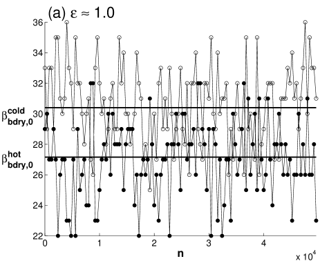
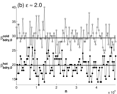
Figure 5: The number of components connected to the boundary for $\epsilon\approx 1.0$ (a) and $\epsilon\approx 2.0$ (b). As in Fig. 2 closed circles represent $X^{hot}$ and open circles represent $X^{cold}$. A sample from every 400th data point from the complete time series is displayed in the above figures.

In summary, we have presented a robust topological characterization of experimental data from a spatiotemporal complex dynamical system. This technique gives one the ability to map the gross global configuration of a state to a few dimensionless numbers. We found stochastic (and ergodic) global topological dynamics for the system of spiral defect chaos where the underlying microscopic dynamics is deterministic and previously observed to be locally chaotic. We also found asymmetric topological configurations between hot and cold regions for which we are unable to provide a physical mechanism. A more complete description of the system would require coupling such scale-independent measures with other measures that depend on the length-scales of the patterns, e.g. the mean length of a roll between defects. Additionally, it would be interesting to compare the correlation of local characterizations such as Lyapunov exponents or wave numbers with variations in quantitative topological measures. Understanding the interplay between local and global dynamics is a core issue in the study of complex systems.

Acknowledgements.— M. G. was partially supported by CAPES, Brazil. K. M. was partially supported by NSF-DMS-0107395. Support by NSF-ATM-0434193 is gratefully acknowledged by K. K. and M. S.

References

- Morris et al. (1996) S. W. Morris, E. Bodenschatz, D. S. Cannell, and G. Ahlers, Phys. D 97, 164 (1996).
- Ecke et al. (1995) R. E. Ecke, Y. Hu, R. Mainieri, and G. Ahlers, Science 269, 1704 (1995).
- Manneville (1990) P. Manneville, Dissipative structures and weak turbulence, Perspectives in Physics (Academic Press Inc., Boston, MA, 1990), ISBN 0-12-469260-5.
- Morris et al. (1993) S. W. Morris, E. Bodenschatz, D. S. Cannell, and G. Ahlers, Phys. Rev. Lett. 71, 2026 (1993).
- Egolf et al. (1998) D. A. Egolf, I. V. Melnikov, and E. Bodenschatz, Phys. Rev. Lett. 80, 3228 (1998).
- Egolf et al. (2000) D. A. Egolf, I. V. Melnikov, W. Pesch, and R. E. Ecke, Nature 404, 733 (2000).
- Settles (2001) G. S. Settles, Schlieren and Shadowgraph Techniques, Experimental Fluid Mechanics (Springer-Verlag, New York, 2001), ISBN 3-540-66155-7.
- Gameiro et al. (2004) M. Gameiro, K. Mischaikow, and W. Kalies, Phys. Rev. E 70, 035203 (pages 4) (2004).
- Kaczynski et al. (2004) T. Kaczynski, K. Mischaikow, and M. Mrozek, Computational homology, vol. 157 of Applied Mathematical Sciences (Springer-Verlag, New York, 2004), ISBN 0-387-40853-3.
- Kalies and Pilarczyk (2003) W. Kalies and P. Pilarczyk, Computational homology program, http://www.math.gatech.edu/~chom/ (2003).
- Busse (1967) F. H. Busse, J. Fluid Mech. 30, 625 (1967).
- Chandrasekhar (1961) S. Chandrasekhar, Hydrodynamic and hydromagnetic stability, The International Series of Monographs on Physics (Clarendon Press, Oxford, 1961).
- Cross and Hohenberg (1993) M. C. Cross and P. C. Hohenberg, Rev. Modern Phys. 65, 851 (1993).