Evidence for strong dynamical evolution in disk galaxies through the last 11 Gyr. GHASP VIII: A local reference sample of rotating disk galaxies for high redshift studies

Abstract

Due to their large distances, high redshift galaxies are observed at a very low spatial resolution. In order to disentangle the evolution of galaxy kinematics from low resolution effects, we have used Fabry-Perot 3D H$\alpha$ data-cubes of 153 nearby isolated galaxies selected from the Gassendi H$\alpha$ survey of SPirals (GHASP) to simulate data-cubes of galaxies at redshift $z=1.7$ using a pixel size of $0.125^{\prime\prime}$ and a $0.5^{\prime\prime}$ seeing. We have derived H$\alpha$ flux, velocity and velocity dispersion maps. From these data, we show that the inner velocity gradient is lowered and is responsible for a peak in the velocity dispersion map. This signature in the velocity dispersion map can be used to make a kinematical classification, but misses 30% of the regular rotating disks in our sample. Toy-models of rotating disks have been built to recover the kinematical parameters and the rotation curves from low resolution data. The poor resolution makes the kinematical inclination uncertain and the position of galaxy center difficult to recover. The position angle of the major axis is retrieved with an accuracy higher than 5^∘ for 70% of the sample. Toy-models also enable to retrieve statistically the maximum velocity and the mean velocity dispersion of galaxies with a satisfying accuracy. This validates the use of the Tully-Fisher relation for high redshift galaxies but the loss of resolution induces a lower slope of the relation despite the beam smearing corrections. We conclude that the main kinematic parameters are better constrained for galaxies with an optical radius at least as large as three times the seeing. The simulated data have been compared to actual high redshift galaxies data observed with VLT/SINFONI, Keck/OSIRIS and VLT/GIRAFFE in the redshift range $3>z>0.4$, allowing to follow galaxy evolution from eleven to four Gyr. For rotation-dominated galaxies, we find that the use of the velocity dispersion central peak as a signature of rotating disks may misclassify slow and solid body rotators. This is the case for $\sim 30$% of our sample. We show that the projected local data cannot reproduce the high velocity dispersion observed in high redshift galaxies except when no beam smearing correction is applied. This unambiguously means that, unlike local evolved galaxies, there exists at high redshift at least a population of disk galaxies for which a large fraction of the dynamical support is due to random motions. We should nevertheless insure that these features are not due to important selection biases before concluding that the formation of an unstable and transient gaseous disk is a general galaxy formation process.

1 Introduction

Formation and evolution of galactic disks is one of the most important unsolved questions of extragalactic astronomy and is probably a key clue to merge cosmological models and galaxy building-up mechanisms. The understanding of the rate and the processes followed by galaxies of different masses to assemble, the relative importance of mergers versus continuous gas accretion infall onto the disk, the connection between bulge and disk formation and more widely the dynamical evolution, the rate of metal enrichment, the evolution of ratio between the baryonic and dark matter masses and mass distribution, the angular momentum transfers during these processes are among some of the fundamental and open questions.

Since the mid 1990s, large ground-based telescopes combined with space observatory multiwavelength observations allow to tackle observationally the question of galaxy formation. The challenges for the future are also to extend the study of galaxy formation to the earliest phases, at $z>6$, and to chart the progress of galaxy formation in detail down to lower redshifts. Morphological and photometric studies point out that high redshift galaxies do not show well-defined shapes and their colors indicate a rapid star formation. Galaxies undergo strong evolution from irregular clumps of star formation into the Hubble sequence valid in the local universe (Papovich et al., 2005). Global properties such as stellar mass, population age, star formation rate, large-scale gaseous outflows, active galactic nucleus fraction have been extensively studied by numerous authors (Dickinson et al., 2003; Steidel et al., 2004; Reddy et al., 2006). The epoch of galaxy formation may span over a broad period probably over 5 Gyrs. At redshifts $z\sim 2$, galaxies are thought to be accumulating the majority of their stellar mass and a wide variety of evolutionary states from young and active star-forming to massive and passively evolving galaxies are observed. At redshifts $z\sim 1$, the pattern of spiral and elliptical galaxies observed in the nearby universe has settled into place even if the fraction of peculiar galaxies is higher (Glazebrook et al., 1995; Abraham et al., 1996; Lotz et al., 2008). However, it is still unknown whether the majority of star formation occurs in flattened disk-like or alternatively in non-equilibrium systems. More widely, it is clear that we do not yet understand the dynamical state of galaxies during this period in which they are forming the bulk of their stars (Law et al., 2007).

More than one thousand high redshift galaxies (mainly Lyman-break galaxies up to $z\sim 3$) have a spectroscopic redshift (e.g. Steidel et al., 2003). Samples of galaxies have been observed with long slit spectrographs to study their kinematics and dynamics. Pioneer observations of $z\sim 1$ disk galaxies have been obtained by Vogt et al. (1996); Vogt et al. (1997). Observations of galaxies at higher redshift were more recently obtained (Erb et al., 2003, 2004, 2006; Weiner et al., 2006; Kassin et al., 2007). Studies using NIR slit or integral field unit (IFU) spectroscopy of H$\alpha$ emission under seeing limited conditions have suggested that at least a subset of high redshift galaxies have a disk-like morphology and show large organized rotation, which may indicate the formation of an early galactic disk (Erb et al., 2003). Kassin et al. (2007) showed from long slit spectroscopy kinematical data and HST restframe B-band morphology that a correlation between peculiar kinematics and peculiar or merger-like morphology exists at $z\sim 1$.

However, at high redshift, the small angular size of the galaxies ($\sim 0.5-1.5$″), comparable to the size of the seeing halo which imposes to set-up a large width for the slit, is a serious observational difficulty. The difficulty is even enhanced by the fact that irregular galaxy morphology may induce possible strong misalignment of the slit with respect to the kinematic major axis. Moreover, with slit spectroscopy, it is not possible to study internal kinematics features like spiral arms or bars. For these reasons, the use of integral field spectroscopy has been overcome using seeing-limited and adaptive optics (AO) assisted integral field unit spectroscopy to obtain two-dimensional maps of these galaxies. Due to obvious observational difficulties, the advent of large telescopes and specialized focal instrumentations were necessary to map in 3D some of these galaxies. Nowadays, kinematics and dynamics of intermediate to high redshift ($0.4<z<3$) galaxies are being increasingly studied with integral field instruments on 8/10-meters class telescopes. IMAGES survey (Flores et al., 2006; Puech et al., 2006; Yang et al., 2008; Neichel et al., 2008; Puech et al., 2008; Rodrigues et al., 2008) contains 63 velocity fields and velocity dispersion maps of intermediate galaxies ($0.4<z<0.75$) observed with the integral-field spectrograph FLAMES/GIRAFFE at the VLT in the optical, in order to probe the dynamical evolution, in particular in the Tully-Fisher relation. The SINS survey has been carried out with the integral-field spectrograph SINFONI at the VLT (Förster Schreiber et al., 2009 and references therein). They have analyzed the 2D H$\alpha$ kinematics for 63 high redshift galaxies ($1.3<z<2.6$) in the near infra-red (among 80 galaxies observed). They realized sub-kpc resolution AO assisted observations using SINFONI for eight galaxies plus four $z\sim 3$ Lyman Break Galaxies. Similar programs are under progress also using SINFONI at redshift $\sim 1.5$ (Epinat et al., 2009b, Queyrel et al., 2009, Contini et al. in preparation) and using OSIRIS at Keck Observatory at redshift $\sim 1.5$ (Wright et al., 2007, 2009) and $z\sim 3$ (Law et al., 2007, 2009).

The question of the assembly of galaxies via major dissipative mergers or internal secular processes has been recently intensely debated in the literature. Based on the analysis of H$\alpha$ velocity fields, velocity dispersion maps and flux distributions, all the different teams advocated that disk candidates are distinguishable from merger candidates. Förster Schreiber et al. (2009) classified the whole SINS sample and concluded that a third of galaxies has rotation-dominated kinematics, another third is composed of interacting or merging systems and the last third has dispersion-dominated kinematics. Epinat et al. (2009b) reached the same conclusions from the MASSIV pilot run. Wright et al. (2009) and Law et al. (2009) gave conclusions compatible with this classification. However, the large picture that emerges in terms of galaxy formation is still a bit confused. Genzel et al. (2008, 2006) and Förster Schreiber et al. (2006) claimed that a secular process of assembly forms bulges and disks in massive galaxies at $z\sim 2$. Robertson & Bullock (2008) nevertheless suggested that the observation of high redshift disk galaxies like the one presented in Genzel et al. (2006) is consistent with the hypothesis that gas-rich mergers play an important role in disk formation at high redshift. Law et al. (2007, 2009) and Nesvadba et al. (2008) argued that galaxies display irregular kinematics more related to merging or gas cooling systems than rotating disks and concluded that the high velocity dispersions observed in most of the galaxies at $z\sim 2$ may be due neither to a ‘merger’ nor to a ‘disk’, but to the result of instabilities related to cold gas accretion becoming dynamically dominant. Epinat et al. (2009b) advocated that several processes are acting at these epochs. Among them, merging seems to play a key role. Close pairs of galaxies expected to merge in less than 1 Gyr, indicate that the hierarchical build up of galaxies at the peak of star formation is fully in progress. The dominant ‘perturbed rotators’ may include a significant fraction of galaxies with minor mergers in progress or cold gas accretion along streams of the cosmic web, producing a high velocity dispersion.

The unusual kinematics, the high gas fraction and star formation rates in high redshift galaxies have been observed quite recently and attempts to explain them have been done. One explanation is that these young galaxies may have experienced gas-rich major or minor mergers (e.g. Semelin & Combes, 2002; Robertson & Bullock, 2008). An alternative or complementary scenario may be that early-stage galactic disks accrete large amounts of low angular momentum gas from the cosmic web and thus content huge quantities of cold gas which fragments and collapses to form violent starbursts (e.g. Immeli et al., 2004b; Bournaud et al., 2007; Elmegreen et al., 2007).

In that last scenario, large star formation may have happened in dispersion-dominated transitory disks rather than in rotationally supported gaseous disks as predicted in current galaxy formation theories. Through secular evolution processes, these unstable disks may lead to the formation of the nowadays bulges and thick disks. Filamentary gas accretion mechanisms should be no more observable nowadays since large amounts of low angular momentum cold gas do not exist anymore. As a consequence, merging is the only mechanism able to fuel galaxies with large amounts of fresh gas in the local universe while at higher redshifts alternative mechanisms may have been in strong concurrence.

Selection effects in the different observations are induced by the relatively low number of galaxies studied and cosmic variance effects. For obvious observational reasons, preferentially extended and bright emission lines galaxies were selected. The prevalence of large velocity shears (large galaxies) or large velocity dispersions (mergers, etc.) in these sources may thus be a product of the selection criteria.

At high redshift, the best seeing-limited observations cover $\sim 5~{}kpc$ and provide only 2 or 3 spatial resolution elements across the major axis of a typical galaxy. Seeing limited studies may miss velocity structures on spatial scales smaller than that of the seeing halo, thus these kinematical measurements are insufficient to claim rotation without using a model to deconvolve the beam smearing effect. The use of IFU instead of long slit spectrograph minimizes the problem but does not solve it completely. Current integral field surveys at redshift $z>0.5$ lack of a reference that would be affected by the same observation and methodological biases. This is for instance necessary to probe a possible evolution in the Tully-Fisher relation or to probe a possible evolution in the dynamical support (rotation or dispersion). A solution is the use of N-body/hydrodynamical simulations of galaxies projected at high redshift as done by Kronberger et al. (2007). A complementary approach, tackled in this work, is to use real data and project them at high redshift, with the same observing conditions as the real high redshift observations.

In section 2 we describe previous simulations of high redshift data from nearby kinematical data. In section 3, we describe the GHASP subsample selection and the simulation of redshifted galaxies. We test the validity of a galaxy classification based on the kinematical maps in section 4. We present the velocity maps analysis method in section 5, we comment the results in section 6, then discuss them in section 7. A conclusion is provided in section 8. The model used to recover the high resolution velocity fields and rotation curves from the projected local data set of galaxies is more widely detailed in Appendix A. The fit parameters and the beam smearing parameter for each galaxy are given in Appendix B. The maps of local sample projected at high redshift are displayed in Appendix C and the rotation curves corresponding to actual data and different models are given in Appendix D. Appendixes B, C and D are provided online only.

Throughrout this paper we use a standard cosmology with $H_{0}=71$ $km~{}s^{-1}$$~{}Mpc^{-1}$, $\Omega_{m}=0.27$, and $\Omega_{\Lambda}=0.73$. We have chosen to project our sample at the critical cosmological scale of redshift 1.7 which is in addition representative of the scale of galaxies from four to eleven Gyr ($0.4<z<3$). In such a cosmology, at redshift $z=1.7$, $1^{\prime\prime}$ corresponds to $8.56~{}kpc$.

2 Local galaxies to simulate distant galaxies

To learn about galaxy evolution, a method is to compare primordial galaxies to nowadays ones. Because of their large distances, high redshift galaxies are obviously not observable with the same spatial sampling as low redshift galaxies. To compare nearby and distant galaxies, it is thus necessary to disentangle distance effects from evolution ones.

Due to the lost of spatial resolution, (i) it is difficult to disentangle rotators from mergers; (ii) the determination of the kinematical parameters (position angle of the major axis, center, inclination, systemic velocities) is more difficult; (iii) the structures within the galaxies (bars, rings, spiral arms, bubbles, etc.) as well as the disk/bulbe/halo mass distributions in the inner regions are smoothed when not erased.

The comparison between nearby galaxies projected at high redshift and observed distant galaxies can help identifying signatures of mergers, kinematical parameters and internal galaxy features and shapes.

Even at low redshift, while the spatial resolution is high enough to allow detailed analysis, controversy may exist on the nature and on the history of peculiar galaxies such as interacting, mergers or starforming galaxies. This is the case for instance for the nearby gas rich Hickson compact group HCG 31 which displays a low velocity dispersion ($\sim 60$ $km~{}s^{-1}$) and an intense star formation rate. Three scenarios have been put forward to explain the nature of this object: (i) these are two systems that are in a pre-merger phase (Amram et al., 2004; Verdes-Montenegro et al., 2005; Amram et al., 2007), (ii) the system is a late-stage merger (Williams et al., 1991) or (iii) it is a single interacting galaxy (Richer et al., 2003). At $z=0.013$, the actual redshift of the group, high spatial and spectral Fabry-Perot observations allow to observe that the broader H$\alpha$ profiles (larger than 30 $km~{}s^{-1}$) are located in the overlapping regions between the two main galaxies (HCG 31 A and C). This clearly maps the shock between the two galaxies and the subsequent starburst regions (Amram et al., 2004, 2007). What would tell us the observations of a compact group like HCG 31 ($z=0.013$) when observed at higher redshift ? To illustrate the answer to this question for this specific compact group, beam smearing effects have been tested by Amram et al. (2008). At $z=0.15$, it becomes already difficult to count how many galaxies are involved in the system and the broadening of the H$\alpha$ profiles would be interpreted as an indicator of rotating disk. This system could thus be catalogued as a rotator instead of a merger (Flores et al., 2006). At $z=0.60$, disentangling the system is a real challenge. This illustrates the difficulty to retrieve the true nature and the history of high redshift galaxies from observations affected by a too small spatial resolution.

As illustrated by the previous example, spatial resampling of nearby galaxies has already been used to simulate distant galaxies in order to interpret integral field data as well as long slit observations (Rix et al., 1997; Weiner et al., 2006; Flores et al., 2006; Puech et al., 2008; Shapiro et al., 2008; Amram et al., 2008), but a systematic comparison has never been done for a large local reference sample.

The systematics induced by the beam smearing effects have been studied in Amram et al. (2008) who have projected the data cube of the galaxies used to study the local Tully-Fisher (TF) relation for CGs (Mendes de Oliveira et al., 2003) at different redshifts. They pointed out several features: (i) high redshift galaxies have smoother rotation curves than local galaxies, a “solid-bodyfication” of the rotation curve is observed; (ii) nothing indicates that the maximum velocity of the rotation curve is reached, leading to uncertainties in the Tully-Fisher relation determination.

In order to analyze the kinematics of high redshift galaxies, control samples of nearby galaxies, with well studied kinematics, are necessary. Compact groups are probably extreme cases difficult to describe even if they have probably been more frequent in the past than nowadays. Close-by interacting galaxies may also lead to inextricable confusion if the separation between the galaxies is not large enough to disentangle the individual galaxies. Star forming galaxies dominated by bright HII regions producing strong winds may also lead to misinterpretation when the spatial resolution is not high enough to access the main mass component. Before studying these difficult kinds of galaxies which will be considered in further works, in the present paper we have considered more quiescent galaxies. We study the smoothing of these signatures by using the GHASP sample in order to simulate high redshift galaxies. The aim of this work is to know whether atmospheric seeing may mask more complex structures than simple flattened disk-like configuration and to test different models enabling to recover the structures and the kinematic parameters.

3 The sample

3.1 GHASP: the local dataset

Fabry-Perot observations from the GHASP survey (Epinat et al., 2008b, c) have been used for this work. The GHASP sample contains 203 local galaxies, mainly isolated spirals and irregulars, observed through their H$\alpha$ line. These data consist of high spectral resolution ($\sim 5-10$ $km~{}s^{-1}$) and seeing-limited data cubes. Nearby galaxies present a broad range of luminosities/masses and morphological types and provide a wide range of kinematical signatures (shape of the velocity fields and of the rotation curves as well as presence of non circular structures like bars, spiral arms, etc.). This sample is thus particularly well adapted to be compared with what is thought to be the ancestors of the actual rotating disks.

We have corrected some local distances computed from the Hubble law using the systemic velocities, since the Hubble constant in the GHASP paper ($H_{0}=75$ $km~{}s^{-1}$$~{}Mpc^{-1}$) differs from the one used in the present paper ($H_{0}=71$ $km~{}s^{-1}$$~{}Mpc^{-1}$).

3.2 The redshifted dataset

153 galaxies belonging to the GHASP sample have been projected to redshift $z=1.7$ and constitute the so-called “redshifted dataset”. We describe in this section the selection criteria and the techniques applied to project the data cubes taking into account several constraints (distance, foreground contaminations, seeing, resampling, etc.) and to compute the moment maps.

3.2.1 Physical length scale

Figure 1: Evolution of the physical length scale with the redshift using the canonical cosmological parameters $H_{0}=71$ $km~{}s^{-1}$$~{}Mpc^{-1}$, $\Omega_{m}=0.27$, and $\Omega_{\Lambda}=0.73$.

Considering the standard cosmology chosen in this paper and ignoring evolutionary effects, the angular size of galaxies decreases with the distance from redshifts $z\sim 0$ to $z\sim 1.7$ and thus increases for redhsifts $z>1.7$ (see Figure 1). We have chosen to set the galaxies at their lower angular size, i.e. at the redshift $z=1.7$ leading to a physical scale of $8.56~{}kpc/arcsec$. This physical scale is representative of high redshift galaxies for which 3D observations are available today. Indeed, the physical scale of $8.56~{}kpc/arcsec$ computed at $z=1.7$ decreases only by $20$% in the range of redshifts $z\sim 0.63-4.34$. Thus, this physical scale correctly matches actual observations of high redshift galaxies done with integral field spectroscopy instruments such as SINFONI (Förster Schreiber et al., 2009), OSIRIS (Law et al., 2009; Wright et al., 2007, 2009) and FLAMES/GIRAFFE (Flores et al., 2006; Yang et al., 2008).

3.2.2 Flux re-scaling

Direct comparison between low and high redshift galaxy fluxes is not straightforward since high redshift galaxies do have higher star formation rates and higher luminosities than at low redshift. Nevertheless, instead of giving arbitrary units for H$\alpha$ fluxes, we have computed the expected flux $F_{l}$ at redshift $z=1.7$ for each galaxy, using the flux $F_{0}$ computed from the calibration in Epinat et al. (2008b), the distance $d$ of the galaxy and the luminous distance at redshift 1.7 ($d_{l}=12.865~{}Gpc$) using equation 1:

$$F_{l}=F_{0}\times\frac{d^{2}}{d_{l}^{2}}$$ (1)

H$\alpha$ monochromatic maps presented in Appendix C have been calibrated using equation 1.

3.2.3 Cleaning from background contaminations

In order to exclude most of the foreground stars from the Milky Way as well as to reduce residual night sky lines contribution, regions where no ionized gas was detected in the local data cubes have been masked on each channel. Indeed, sky contribution is large since it is integrated over a large angular size (around 10′ square).

3.2.4 Blurring, resampling and noise addition

The wavelength range of the data cube has been extended from 24 to 72 channels in order to remove interfringe effects due to the spectrum periodicity of Fabry-Perot interferometers (Epinat, 2008a). Each channel of the cube has been blurred by a two dimensional gaussian simulating the seeing. The width of this gaussian has been computed taking into account the seeing measured on the $z=0$ data so that the seeing halo for redsfhited galaxies is simulated by a two dimensional gaussian function of 0.5″ FWHM. This halo of 0.5″matches the best average spatial resolution that can be reached without AO. This operation is computed in the Fourier space.

The spatial sampling has been set to 0.125″, to mimic the SINFONI pixel size. To avoid any interpolation, the binning is the merging of an integer number of real pixels that corresponds to the closest simulated size obtained for a redshift $z=1.7$. The ratio seeing/pixel size has been set to be identical for each galaxy. Thus the mean scale for our sample is $8.5~{}kpc/arcsec$ with a standard deviation of $0.3~{}kpc/arcsec$.

In the present study, no spectral binning or smoothing has been applied in order to dissociate these two resolution effects on 3D data (this test will be done in a forthcoming work).

No noise has been added in the datacubes. Our goal is to study the beam smearing effects in the data to test the ability to recover the kinematical parameters. Indeed, if noise is added on the spectra simultaneously to blurring, it will not be straightforward to unambiguously disentangle the lack of spatial resolution from the low signal-to-noise ratio. Adding noise reduces the detectability at low intensity levels, does not strongly bias velocity distribution but affects velocity dispersion measurements. The signal-to-noise ratio of the simulated data (ranging from $\sim 3$ to $\sim 50$) is higher than real high redshift observations (ranging from $\sim 2$ to $\sim 10$, e.g. Epinat et al., 2009b). The signal-to-noise ratio slightly varies from one galaxy to the other since the binning is not the same.

3.2.5 Cleaning procedures on redshifted data

A cleaning procedure has been applied on redshifted data to remove spurious measurements outside of the galaxies. We used the following criteria that ensure to avoid discontinuities on the edges of the velocity fields: the velocity dispersion must be larger than 5 $km~{}s^{-1}$, which is lower than the spectral resolution of our data, and the signal-to-noise ratio (defined as the ratio of the H$\alpha$ monochromatic flux over the RMS among spectral elements in the continuum at that pixel times the full width of the line) must be larger than 2.7. This cleaning corresponds to the maps presented in Appendix C.

3.2.6 Computating the moment maps for redshifted data

The different maps have been computed using the barycenter method described in Daigle et al. (2006) and already used to compute the local maps in Epinat et al. (2008b, c). Velocity dispersion maps heve been corrected from the spectral PSF considered to be described by a gaussian function using the following classical relation:

$$\sigma^{2}_{corr}=\sigma^{2}_{obs}-\sigma^{2}_{PSF}$$ (2)

3.2.7 Selection of a sub-sample

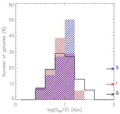
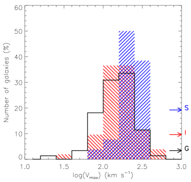
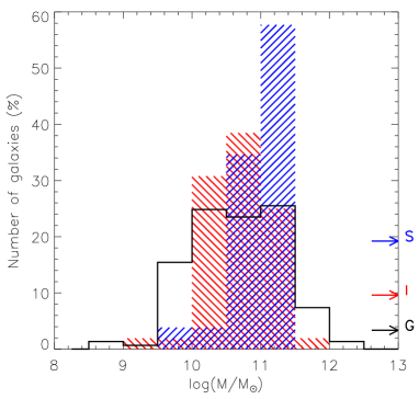
Figure 2: Relative distribution of galaxy properties. Top: optical radius; Middle: maximum rotation velocity; Bottom: masses. The black stairs indicates the GHASP local sub-sample, the red hatchings the IMAGES sample and the blue hatchings the SINS sample. In order to show the respective size of the samples (153, 63 and 26 galaxies respectively for GHASP, IMAGES and SINS), arrows and letters with the same colors indicate five galaxies for each sample (G for GHASP, I for IMAGES and S for SINS).

To avoid artifacts and to produce a realistic sample, only a sub-sample of GHASP galaxies has been used to simulate galaxies at high redshift. Some galaxies coming from the GHASP sample have been rejected. The selection criteria are described hereafter.

I. Actual observations of high redshift galaxies are limited in flux and in size. We have discarded too small and too faint galaxies and “uncomplete” observations:

(i) galaxies with an optical radius smaller than $3.2~{}kpc$ ($3/4$ of the seeing at $z=1.7$);

(ii) galaxies having less than 20 pixels after cleaning;

(iii) galaxies with an integrated H$\alpha$ emission fainter than $10^{-22}~{}W~{}m^{-2}$;

(iv) “uncomplete” observations, i.e. galaxies larger than the field-of-view (see Epinat et al., 2008b) (for which H$\alpha$ emission is missed, the comparison has been made with H$\alpha$ images when available from NED database) as well as galaxies showing a non uniform H$\alpha$ emission due to filter transmission problems.

II. Pair galaxies are analyzed separately when their angular separation at high redshit is large enough (typically 0.5″) to clearly disentangle them. Only the two pairs UGC 5931/5935 and UGC 8709/NGC 5296 are presented on the same maps in Appendix C. Only UGC 8709 is analyzed since it is clear on projected maps that NGC 5296 is only a small satellite. The pair UGC 5931/5935 is the only one that could be interpreted as a single galaxy at redshift $z\sim 1.7$ thus the couple is analyzed as a single galaxy, UGC 5931.

In summary, the sub-sample resulting from these criteria contains 153 galaxies (or close pair galaxies) among the 203 GHASP galaxies. Thus, our sample contains 153 simulated high signal-to-noise ratio, high spectral resolution ($\sim 10$ $km~{}s^{-1}$), sky subtracted data cubes of galaxies observed at a redshift $z\sim 1.7$ under good seeing conditions ($0.5^{\prime\prime}$ seeing) with a $0.125^{\prime\prime}$ spatial sampling.

Some examples of the original and blurred maps are given in Figure 3: for each galaxy, the top line presents the actual maps already presented in Epinat et al. (2008b, c) whereas the bottom one corresponds to the blurred maps for the same galaxy projected at redshift $1.7$. The whole set is presented in Appendix C: the original XDSS image, as well as the blurred H$\alpha$ flux, velocity field and the velocity dispersion maps are given for each galaxy of the sub-sample. On each map of Figure 3 and Appendix C, the white and black double crosses mark the center used for the analysis while the black line represents the major axis used or derived from the analysis. This line ends at the optical radius taken from the RC3 catalog (see Table LABEL:table_modz0).

In Appendix D, we present the rotation curves of redshifted galaxies. The black dots correspond to the rotation curve along the major axis (determined from high resolution data, see Table LABEL:table_modz0). The velocities are measured on the velocity field for the pixels intercepted by the major axis and are deprojected from inclination. The colored lines are the high resolution rotation curves obtained from the models fit on the velocity fields (see section 5). The red-open triangles correspond to the high resolution rotation curves from Epinat et al. (2008b, c). These authors have computed the rotation curves from H$\alpha$ data cubes obtained from adaptive binning techniques based on Voronoi tessellations. Original improvements, based on the whole 2D velocity field and on the power spectrum of the residual velocity field rather than the classical method using fit in annuli or tilted ring model has been used to compute the rotation curves. The kinematical parameters (inclination, position angle, systemic velocity and center) were not allowed to vary with the radius.

3.2.8 Distribution of the sub-sample

Figure 2 presents the relative distribution for the three following galaxy parameters: optical radius ($D_{25}/2$), maximum rotation velocity ($V_{max}$) and total mass ($M$) computed within the optical radius for three different samples.

$$M=\frac{V_{max}^{2}\times~{}D_{25}/2}{G}$$ (3)

These samples are: (i) the GHASP sub-sample previously defined (black stairs); (ii) the IMAGES sample (red hatchings) observed with FLAMES/GIRAFFE (Flores et al., 2006; Puech et al., 2006; Yang et al., 2008; Neichel et al., 2008; Puech et al., 2008) and (iii) the 26 galaxies from SINS sample (blue hatchings) for which these measurements are available so far, and that are mainly classified as rotating disks (Förster Schreiber et al., 2009; Cresci et al., 2009). For comparison, the total amount of galaxies of each sample being different (153 for GHASP, 63 for IMAGES and 26 for SINS), we have marked on the histograms of Figure 2 a reference level of five galaxies for each sample with arrows of the same color as the histograms (G for GHASP, I for IMAGES and S for SINS). The GHASP local sample contains galaxies over a broader mass range resulting from larger galaxies and slowest rotators than the two other samples. The lack of very large galaxies at high redshift can be explained by both evolution effect and observational biases due to a poorer signal-to-noise ratio, inducing underestimated radii. We may also notice that GHASP barred galaxies are on average smaller than unbarred galaxies. This biases the comparison that can be done between barred and unbarred galaxies since we expect the parameters determination accuracy to be correlated with the size of redshifted galaxies. The bias induced between barred and unbarred GHASP galaxies does not affect the global comparison with high redshift galaxies. Moreover, even if high redshift and local distributions are different, the simulated maps are suited for studying biases in the kinematical parameters determination since the GHASP sub-sample covers the whole mass, extent and velocity ranges observed at high redshift. It is however interesting to notice that almost no high redshift galaxies from both IMAGES and SINS samples are slow rotators even if they are on average smaller objects. This is probably due to magnitude selection effects and could indicate that no H$\alpha$ is detected in the outer regions (nevertheless, Cresci et al., 2009 found a good agreement between the radii measured in $K$-band and in H$\alpha$). Moreover, high redshift samples are not selected in a statistically complete way since they aim at observing galaxies with resolved kinematics.

UGC 07901 (unambiguous case)	UGC 05414 (i)
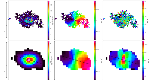
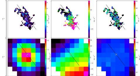
UGC 07853 (ii)	UGC 05789 (iii)
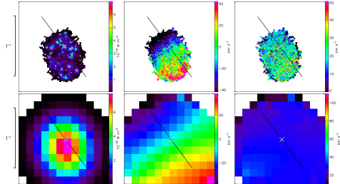
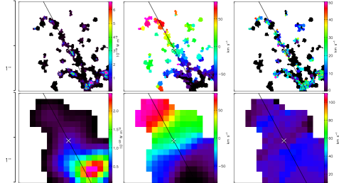
UGC 10310 (iv)	UGC 04820 (v)
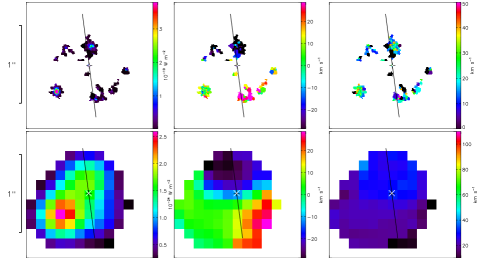
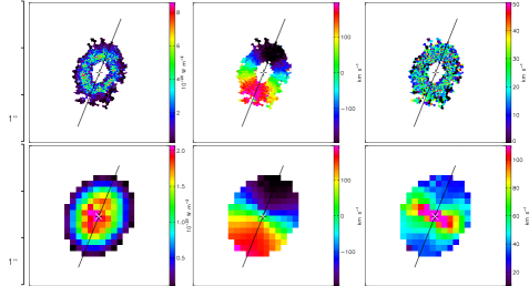
UGC 05556 (vi)	UGC 05931 (vii)

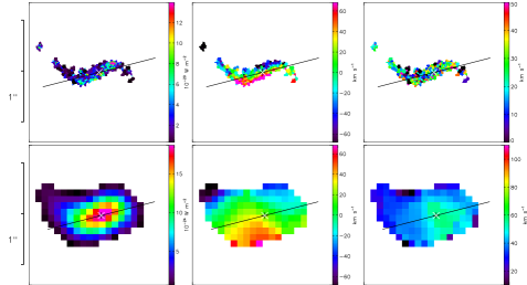
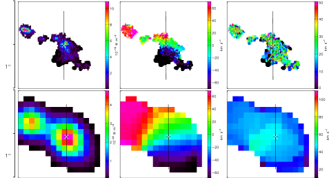
Figure 3: Spatial resolution effects illustrated on eight galaxies illustrating an unambiguous case and the cases described from (i) to (vii) in section 4. The following comments concern each galaxy. Top line: actual high resolution data at $z=0$. Bottom line: data projected at $z=1.7$. The spatial scale is labelled in arcsecond on the left side of both lines. From left to right: H$\alpha$ monochromatic maps, velocity fields and velocity dispersion maps. The rainbow scale on the right side of each image represents the flux for the first column and the line-of-sight velocities corrected from instrumental function for the two next columns. The black and white double crosses mark the kinematical center at low redshift, while the black line represents the major axis and ends at the optical radius. More projected galaxies are presented in Appendix C.

3.2.9 Velocity field extent

As already underlined in paragraph 3.2.4, our redshifted sample benefits from a high signal-to-noise ratio, thus, our velocity fields are probably more extended than what observation facilities would enable for real high redshift observations. The extent of local velocity fields is close to the optical radius value as underlined by Garrido et al. (2005). The mean value of optical radius for our GHASP sub-sample is $11~{}kpc$ (median value is $9~{}kpc$), with a dispersion of $7~{}kpc$. The lowest value is $3~{}kpc$ and the highest value is $35~{}kpc$. For comparison, we have converted half light radii ($r_{1/2}$) taken from the literature for high redshift objects into optical radii ($r_{opt}$) assuming an exponential distribution of light: $r_{opt}=1.9r_{1/2}$.

IMAGES galaxies observed with FLAMES/GIRAFFE in the redshift range $0.4<z<0.75$ by Neichel et al. (2008) have a mean optical radius of $9~{}kpc$ with a scatter of $\pm 4~{}kpc$, which is comparable to our sample. Their smallest galaxy is $2.9~{}kpc$ and the largest is $19.5~{}kpc$. On average, the 16 galaxies observed with OSIRIS by Law et al. (2009) with redshifts from 2 to 3 extend up to $1.1\pm 0.3~{}kpc$. These values are very low. This could be partially attributed to the different estimators. Indeed, the disk dimensions are deduced from the ionized gas flux map, which is not completely suitable for comparison. The four $z\sim 1.5$ redshift galaxies observed by Wright et al. (2007) with OSIRIS using AO extend up to $4.9\pm 1.1~{}kpc$ in optical radius. Förster Schreiber et al. (2006, 2009) and Cresci et al. (2009) have provided half light radius measurements for 26 galaxies (mainly for rotating disks) out of the 63 SINS galaxies. The mean optical radius is $9.1\pm 3.3~{}kpc$, the smallest galaxy radius is $3.2~{}kpc$ and the largest one is $14.5~{}kpc$, which is still slightly smaller than for the GHASP sample. The nine galaxies with redshift ranging between 1 and 1.5 presented by Epinat et al. (2009b) have optical radii of $10.3\pm 4.1~{}kpc$. The sizes are ranging from $5.3~{}kpc$ to $17.3~{}kpc$. Except for high redshift galaxies observed with the OSIRIS instrument that uses AO facility (Law et al., 2009; Wright et al., 2007, 2009), the extent of high redshift galaxy velocity fields is rather similar to the ones of our sub-sample. However, there is no case for galaxies larger than $20~{}kpc$ as already noticed from the histogram in Figure 2. The smaller extent of observations with AO facility could be explained by the use of a very small pixel scale (50 mas for both OSIRIS and SINFONI in AO mode) that induces a loss in flux detection. Indeed, for constant surface brightness objects, it is necessary to use longer exposures when using a smaller pixel scale to reach a given signal-to-noise ratio, even with a negligible read-out noise.

On the other hand, due to selection criteria effects on high redshift sample, we would expect to observe large galaxies but evolution processes have the opposite effect. In conclusion, since local data have a better signal-to-noise ratio and on average a larger spatial extent, in section 6, we have truncated the images of all the galaxies at the optical radius to mimic high redshift galaxies. However, the maps presented in Appendix C are not truncated.

3.3 Biases induced by spatial resolution effects

At redshift $z=0$, the use of optical spectroscopy is the best way to probe the inner shape of rotation curves since the inner regions are usually not well resolved with HI radio observation (for GHASP data already observed in HI in the WHISP survey by Noordermeer et al., 2005, the typical resolution is $\sim 5~{}kpc$). Optical rotation curves are not always extended enough to determinate reliable maximum velocities (Garrido et al., 2005). Complementarily, HI data are used to trace the outer regions of rotation curves since HI generally extends further away. At high redshift, the situation regarding the spatial resolution in optical or in infrared becomes comparable to HI at local redshift, but still with a smaller extent. Thus, the biases due to spatial resolution effects for our sample are somewhat similar to HI beam smearing effects for local galaxies (see section 6.1 for a discussion on the beam smearing parameter). Our projected sample gives a good opportunity to revisit these biases, and to point out specific biases in the optical or in the infrared since we exactly know how the high resolution kinematical maps look like.

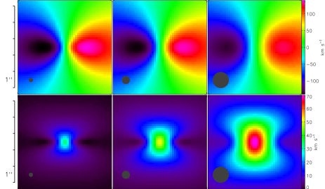
Figure 4: Beam smearing effects on a simulation (velocity fields on the top line and velocity dispersion maps on the bottom line) depending on increasing blurring parameter. From left to right, the seeing (represented by a dark disk on the six images) increases from 0.25″ to 1″. The pixel size is 0.125″. The disk scale length is set to 5 kpc (observed at $z=1.7$), the inclination is 45^∘ and the maximum velocity in the plane of the disk is 200 $km~{}s^{-1}$.

From the comparison between the original and redshifted maps given in Figure 3 in the case of UGC 07901 (top-left), we note that:

(i) The apparent size of the galaxy seems to be enlarged while in fact, flux limits reduce it. Indeed, the emitting regions in the blurred images are artificially extended toward outer regions of the galaxy where there is in fact no emission. This is due to beam smearing that spreads out the flux over the PSF. In actual observations, depending on the signal-to-noise ratio, these faint outer regions should not exist.

(ii) Concerning the H$\alpha$ monochromatic map, we totally lose the details of the inner ring distribution and the emission is only present in the central peak of the blurred images.

(iii) The velocity gradient is lowered along the major axis while the velocity gradient is increased across the minor axis. Indeed, both velocity fields nevertheless present the usual “spider” shape. However, the isovelocity lines are more open for the high redshift galaxy than for the $z=0$ galaxy. If one does not take into account the beam smearing, this could be interpreted as a lower inclination for the redshifted galaxy (the same conclusion would be reached by looking at the morphology due to the fact that the relative enlargement is higher for the minor axis than for the major axis).

(iv) The velocity dispersion maps are quite different. The bottom-right map shows the velocity dispersion affected by beam smearing, the top-right map displays the velocity dispersion for each point of the galaxy, referred hereafter as the local velocity dispersion and noted $\sigma$. We aim to measure this quantity in order to estimate the pressure support for both nearby and distant galaxies. The local velocity dispersion does not display any strong feature whereas the velocity dispersion map at high redshift clearly shows a central peak elongated along the minor axis. As already discussed by other authors (e.g. Weiner et al., 2006; Flores et al., 2006), this peak is only due to beam smearing effects: for each pixel, the resulting line is the combination of lines at various wavelengths (velocities) weighted by the real flux and is thus enlarged. The enlargement is maximum where the projected velocity gradient is the highest (see Appendix A for details).

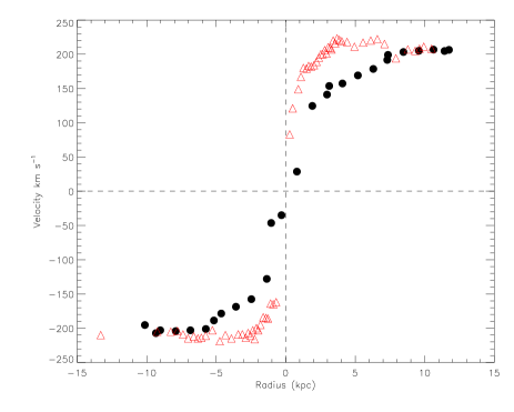
Figure 5: Example of a rotation curve obtained for a redshifted galaxy. Both rotation curves have been computed from both local and projected UGC 7901 velocity fields presented in Figure 3: red-open triangles correspond to local full resolution data while black dots come from the data projected at $z=1.7$.

Both redshifted velocity field and velocity dispersion map contain information on the true velocity field itself. In Figure 4, in order to illustrate this effect that is responsible for both points (iii) and (iv), an exponential disk model has been drawn in order to compute velocity fields and velocity dispersion maps with increasing seeing ranging from 0.25″ to 1″. The disk scale length has been set to $5~{}kpc$ and the maximum velocity of the rotation curve to 200 $km~{}s^{-1}$. The inclination has been fixed to 45^∘. The flux contribution follows an exponential disk, and the local velocity dispersion $\sigma$ is null everywhere. We observe that the velocity shear vanishes whereas the velocity dispersion peak increases. The behavior would be the same with an increasing pixel size or with a decreasing disk scale length. If the local velocity dispersion has a constant value $\sigma$ in the field, the resulting velocity dispersion map is the quadratic sum of $\sigma$ with the previously computed blurred velocity dispersion map. It results that the peak is more attenuated for galaxies with a high local velocity dispersion.

In addition to these effects on the maps, the beam smearing will modify the shape of the rotation curve, which will eventually look like a solid body rotation curve. This is illustrated in Figure 5 where the rotation curve at low redshift (red-open triangles) is over-plotted on the rotation curve derived from the major axis of the redshifted velocity field (black dots). At high redshift, the inner velocity gradient is lowered whereas the outer gradient becomes higher. It can be noticed that the maximum velocity seems to be reached at larger radii (around $8~{}kpc$ instead of $3~{}kpc$) on both the velocity field and the rotation curve of the projected galaxy. This is due to the fact that, for this specific ring galaxy, the blurred H$\alpha$ distribution is dominated by the contribution of the ring. Since it is close to the center, the velocity of the ring has a strong weight and is reached rapidly. At larger radii, the contribution of the H$\alpha$ ring remains important and tends to lower the plateau. For most of the nearby galaxies observed at high spatial resolution with a flatter H$\alpha$ distribution, the inner slope is also shallowed (see Appendix D, e.g. UGC 11872). For galaxies with a lower extent, the maximum velocity is not reached on the rotation curve (see Appendix D, e.g. UGC 528). With HI data at low redshift, this would not be true since, the extent being larger, the external plateau could be reached. However, mostly for massive spiral galaxies, we see that the maximum velocity is reached close to the center in H$\alpha$, the rotation curve may even be decreasing afterward. Epinat et al. (2008c) suggested that this could be a possible explanation for the difference observed in Tully-Fisher relations obtained from H$\alpha$ and HI data for the most massive galaxies.

4 Kinematical signatures of high redshift rotating disks

4.1 Kinematical classification

The velocity dispersion map feature discussed in the previous section is typical of a rotating disk with a rather uniform flux distribution and with a projected velocity gradient larger than 100 $km~{}s^{-1}$, due to the strong inner velocity gradient. Flores et al. (2006) use this signature to provide a dynamical classification for high redshift galaxies (for $z\sim 0.6$): “rotating disks” present a central velocity dispersion peak, “perturbed rotators” show a peak (slightly) offset from the center and objects having “complex kinematics” (e.g. mergers) display featureless velocity dispersion maps. The GHASP sample contains mainly rotating disks, thus we can use it to probe this classification. We find that around 70% of the sample would be correctly classified (i.e. entering in the category “rotating disks”). Nevertheless, the remaining fraction of the sample would be misclassified for the following reasons (see Figure 3 for illustrations of each case):

(i) disks in rotation with a low velocity gradient (face-on, low mass galaxies, high velocity dispersion in the velocity field with respect to the rotation velocity amplitude) show a very faint or no central velocity dispersion peak (see Appendix C, e.g. UGC 3685, UGC 3851, UGC 5414 -Fig. 3-, UGC 6628, UGC 11557);

(ii) disks showing a solid body rotation curve have the same velocity gradient everywhere in the field and thus no peak of velocity shear can be observed in the velocity dispersion map (see Appendix C, e.g. UGC 6419, UGC 7853 -Fig. 3-);

(iii) asymmetries in the H$\alpha$ distribution can induce an offset velocity dispersion peak (hence misclassified as “perturbed rotators”) since the resulting velocity dispersion map is the combination of velocity field shears weighted by the H$\alpha$ monochromatic flux (see Appendix A and Appendix C, e.g. UGC 4393, UGC 5316, UGC 5789 -Fig. 3-);

(iv) galaxies with a patchy H$\alpha$ emission seem to have a continuous emission once projected at high redshift from which can result peculiar velocity fields and velocity dispersion maps (see Appendix C, e.g. UGC 10310 in Fig. 3);

(v) a central hole (or ring) in the flux distribution can be completely blurred depending on the actual size of the galaxies (see Appendix C, e.g. UGC 3382, UGC 4820 -Fig. 3-, UGC 5045);

(vi) the presence of a strong bar can induce very peculiar velocity fields with an apparent position angle of the major axis completely biased (see Appendix C, UGC 5556 being the most impressive case -Fig. 3-);

(vii) using only broad band images, very close pairs (see Appendix C, e.g. UGC 5931 & UGC 5935 in Fig. 3) can appear as a single galaxy with two main clumps. Kinematical data are helpful to distinguish single galaxies from systems composed by two or more galaxies. A paired galaxies system or even a compact group of galaxies may look like a single perturbed galaxy when they are in fact composed of distinct galaxies in interaction or just seen close in projection on the sky plane. Reciprocally, chaotic single galaxies composed by bright clumps may look like multiple systems. In a given field-of-view, multiple galaxies can be identified using the discontinuities in the velocity gradients, the variation of the major axis position angle and the possible multiple components along the line-of-sight in the line profiles (e.g. Amram et al., 2007). Velocity discontinuities are obvious when the different galaxies are rotating in apparent opposite directions but are also visible when the galaxies are rotating with the same apparent spin. Within a given pixel, multiple components in the line profiles can be identified by the relative difference in velocities and often also by difference in flux ratio. In the case of UGC 5931/35 the velocity field looks disturbed even though the actual velocity field is more regular, the position angle of the major axis is biased and the velocity dispersion signature of a rotating disk is partly lost.

In addition to these effects, this classification cannot be used for galaxies with a high local velocity dispersion since the peak in the velocity dispersion map is smoothed.

4.2 IMAGES classification

GIRAFFE observations, in the frame of the IMAGES program (Yang et al., 2008; Neichel et al., 2008; Puech et al., 2008; Rodrigues et al., 2008), provided a sample of 63 galaxies (including those of Flores et al., 2006 and Puech et al., 2006) ranging from $z=0.4$ to $z=0.75$ representative of the population of emission line galaxies more massive than $1.5\times 10^{10}M_{\odot}$ (see Figure 6 in Yang et al., 2008). In this sample, Yang et al. (2008) found 32% of regular “rotating disks”. A lower limit of the number of “anomalous kinematics (pertubed and complex)” galaxies can be given considering that absorption line galaxies are not perturbed. Yang et al. (2008) estimated that absorption line galaxies represent 40% of the total population of galaxies at $z\sim 0.6$. Thus, taking into account all the galaxies (emission and absorption line galaxies) in that redshift range, these authors found that at least $41\pm 7$% of them have anomalous kinematics (not relaxed), including $26\pm 7$% with complex dynamics (not simply pressure or rotationally supported). The merger hypothesis is favored by these authors to explain this complex dynamics. Even if the condition of projection of the local GHASP sample of galaxies presented in this paper is built to match the SINFONI observations rather the GIRAFFE ones, a comparison between local galaxies and galaxies at intermediate redshift (IMAGES/GIRAFFE) may also be done. Indeed, the seeing conditions (without AO) are statistically the same, the sizes of the galaxies do not dramatically differ between redshift $z=1.7$ and $z=0.6$ (at $z=1.7$, 1″$\sim$ $8.6$ kpc and at $z=0.6$, 1″$\sim$ $6.7$ kpc, see Figure 1), the main difference is the sampling of the seeing on the CCD, the one of SINFONI ($0.125$″) being approximately four times higher than that of GIRAFFE ($0.52$″). Nevertheless, the spectral sampling is higher in GIRAFFE ($22-30$ $km~{}s^{-1}$) than in SINFONI ($67-160$ $km~{}s^{-1}$) but lower than in GHASP ($\sim 17$ $km~{}s^{-1}$). On the one hand, from the comparison between IMAGES and GHASP, it can be concluded that actual disks in rotation with emission lines at intermediate redshift look like local disks in rotation projected at high redshift but the absence of perturbed disks in the local sample does not allow to conclude if perturbed disks at intermediate redshift look like perturbed local galaxies. On the other hand, due to the items developped in section 4.1 (ordered from the most to the least relevant), we have shown that 30% of the rotating disks may be misclassified using the classification given by Flores et al. (2006). At high redshift, this is particularly critical for galaxies where noise in the outer parts of the velocity field causes off-center dispersion peak. The “corrected” number of rotating disks in IMAGES sample of 63 galaxies may be underestimated by a factor 1.4. In other words, the fraction of rotating disks found in IMAGES may pass from 32% (see above) to 44%. Reciprocally, the fraction of galaxies with anomalous kinematics for the total population, including absorption and emission line galaxies, may thus be lowered from 41% (see above) to 33%. This gives a lower limit to the fraction of galaxies having anomalous kinematics. Indeed, it is likely that a fraction of absorption line galaxies ara perturbed and also have anomalous kinematics. In addition, based on the observed dynamics in the IMAGES survey and the possible misclassification due to the faint spatial sampling (no AO and large pixel scale) combined to the small spatial coverage (due to the small sizes of the galaxies) and the low SNR in some cases, the anomalous kinematics and even the complex dynamics for several galaxies could be due to unrelaxed gas disk without involving, in all the cases, a merger. Indeed, Liang et al. (2006) estimated that the gas content in intermediate galaxies at $z\sim 0.6$ was twice larger than in galaxies at the current epoch and that one cannot exclude transient episodes of intense gas accretion making the disk unstable during a relatively short period.

To conclude, the kinematical classification made by Flores et al. (2006) is relevant for a reasonable fraction of rotating disks, assuming that the local velocity dispersion is lower than the rotation velocity. However, low velocity gradient in the velocity field, solid body shape for the rotation curve, flux asymmetries in the H$\alpha$ distribution and other asymmetries like strong bars could cause the IMAGES sample to look more pertubed than it actually is.

5 Fitting method

5.1 General model

To recover the actual kinematic parameters (those from high resolution data) through the degenerate blurred data cube, it is absolutely necessary to model the blurred data. Models consisting in a thin planar disk have been used to retrieve (i) the projection parameters (inclination $i$ with respect to the line of sight, position angle of the major axis $PA$ and systemic velocity $V_{sys}$) and (ii) the kinematical parameters (center of rotation, rotation velocity and local velocity dispersion $\sigma$ both as a function of the radius). No hypothesis is done on the nature of the gravitational support (rotation or pressure). The only assumption we do is that the gaseous disk is infinitely thin without any supposition on the amplitude of the velocity dispersion. To constrain the kinematical parameters, this general model allows the use of the blurred velocity fields alone, the blurred velocity dispersion maps alone or the combination of both.

5.2 Method used

In the following, we have only used the blurred velocity fields. A discussion on this choice is provided in section 5.4. The velocity field is supposed to be axisymmetric and the rotation curve is described by two parameters: the maximum velocity of the model $V_{t}$ and a transition radius $r_{t}$. To avoid any $a~{}priori$ shape for the rotation curve describing the redshifted data, we have tested four different models of rotation curve in order to evaluate which ones describe at best the data. These four models all have two free parameters ($r_{t}$ and $V_{t}$). We have chosen rotation curves that have been used for such studies in the literature and which may have rising, flat or decreasing shape: (1) an exponential disk as used for the SINS sample (Cresci et al., 2009); (2) an isothermal sphere as used in mass models (Spano et al., 2008); (3) a model described by an inner linear slope to reach $V_{t}$ and a plateau after $r_{t}$ (referred hereafter as “flat model”) as used for OSIRIS data (Wright et al., 2007, 2009); and finally (4) a model described by an arctangent function as used for the IMAGES sample (Puech et al., 2008). The two first models may have a physical meaning, the two last are well known to fit rotation curves of local galaxies. Except for the arctangent model, the maximum velocity of the model $V_{t}$ is reached at the transition radius $r_{t}$. Ideally, to increase the flexibility of the fit, it should be useful to use a rotation curve described by three parameters, but the addition of one more parameter makes the fit difficult to converge since the number of free parameters is already of the same order than the number of data measurements. These models are described in Appendix A (section A.5) and illustrated in Figure 6 (using $r_{t}=11~{}kpc$, $V_{t}=190~{}km~{}s^{-1}$ and $i=45$^∘). In Appendix D, we have over-plotted the four models to the rotation curves (exponential disk in red, isothermal sphere in green, “flat model” in black, and arctangent function in blue). Thus, the global model contains seven parameters ($i$, $PA$, $V_{sys}$, $V_{t}$, $r_{t}$ and the center coordinates). They are determined from a Levenberg-Marquardt nonlinear least-squares $\chi^{2}$ minimization (Press et al., 1992) and the statistical errors of the fits have been used (see Tables LABEL:table_modzexp to LABEL:table_modzata). Since a simple thin rotating disk model is not suited for the description of highly inclined disks, we set an upper limit of $80$^∘ to the inclination. Moreover, due to the degeneracy between the velocity and the inclination, we set a minimum inclination of $10$^∘ to avoid unrealistically high rotation velocities. It results that 16 galaxies have been excluded from the fitting and thus only 137 out of the 153 galaxies of our sub-sample have been used for the studies presented hereafter.

5.3 Computing method and limitations

From the model parameters previously defined, a high resolution velocity field model is created. Then, the seeing has to be taken into account. In order to do that, ideally, one should know the high resolution line flux map and create a high resolution data cube. Indeed, the line flux weights the contribution of each high resolution spatial element. From observations, it is not yet possible to know the high resolution line flux map. One solution is to use flux distribution models. However, the GHASP local dataset shows that such assumption is abusive since some galaxies display rings, asymmetry or holes. An other solution would be to perform deconvolution from the observed maps. In this study, we simply use the low resolution line map that we interpolate. The method we adopted is more robust than deconvolution technics, but will not recover holes, rings, asymmetries, etc. However, the seeing blur will decrease their effect. Creating a model data cube is a time consuming task. It is possible to avoid the creation of high resolution data cubes by assuming that the H$\alpha$ line is locally well described by a gaussian. This formalism enables to compute directly the blurred velocity field and velocity dispersion map from the seven parameters of the model and is equivalent to generate high resolution data cubes that also need the same assumption. Analytical details are presented in Appendix A. In equation 33, giving the expression of the blurred velocity dispersion, the first term represents the local velocity dispersion contribution whereas the second term corresponds to a velocity shear feature induced by beam smearing effects.

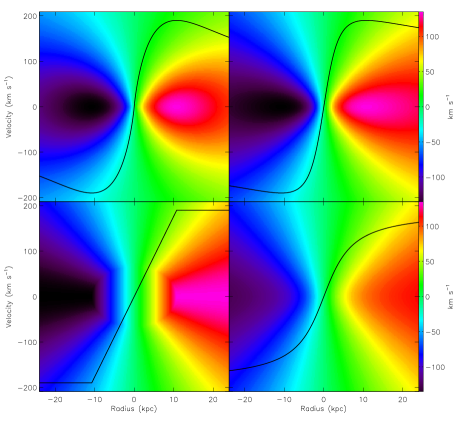
Figure 6: High resolution rotation curves (black curve) superimposed on velocity fields (color image) of the four models used. From left to right and from top to bottom: exponential disk, isothermal sphere, “flat” and arctangent models. The radius (x-axis) is common for the four velocity fields and the four rotation curves. The velocity fields scale is given by the rainbow scale on the right side of the images. The velocity amplitude of the rotation curves is given by the scale on the left side of the y-axis.

5.4 Local velocity dispersion maps

To constrain the kinematical parameters, the generic model presented in section 5.1 allows the use of the blurred velocity fields alone, the blurred velocity dispersion maps alone or the combination of both. In the forthcoming analysis, the kinematical model has been constrained using the blurred velocity fields only. Indeed, the blurred velocity dispersion maps do not add any constraining power, thus, adding a dispersion parameter to the model is not necessary to fit the data. In a second step, the model has been used to correct the beam smearing effects in the velocity dispersion map (see Appendix A).

To demonstrate that the use of the velocity dispersion map is not necessary to constrain the kinematical parameters, we have attempted to combine it to the velocity field in order to retrieve the parameters of the model. In order to model the expected local velocity dispersion map  an additional hypothesis concerning the physical nature of the velocity dispersion is needed. We may choose the local velocity dispersion to be constant (i.e. the same value everywhere in the plane of the galaxy). This hypothesis, being a possibility since it is mainly what is observed in the GHASP sample (Epinat, 2008a, Epinat et al., in preparation), leads to a satisfying agreement with the parameters of the local sample. However, if this method works for the GHASP sample, this is mainly due to the fact that, for nearby galaxies, the velocity shear is high with respect to the local velocity dispersion and the signal-to-noise ratio is high. This might not be the case for distant galaxies for which the signal-to-noise ratio is lower and for which the physical nature of the velocity dispersion is unknown. In addition, even if the method using an unique and constant velocity dispersion works, it not necessary since (i) this parametrical approach needs the introduction of one or more parameters to describe the local velocity dispersion map (radial and azimuthal dependencies, etc.); (ii) the projection parameters and the velocity gradient can be recovered using the velocity field alone; (iii) the constant velocity dispersion could also be retrieved from the velocity field only (see equation 33); (iv) the velocity shear cannot be constrained efficiently when lower than the local velocity dispersion and (v) from a technical point of view, the low signal-to-noise ratio affects more strongly the velocity dispersion (second order momentum) than the velocity (first order momentum) and this would lead to larger uncertainties, in particular for the velocity determination.

To summarize, we favor the method using the velocity field alone since it allows to avoid any a priori hypothesis on the local velocity dispersion. The velocity dispersions are corrected from beam smearing effect using the parameters of the model.

5.5 Residual maps of nearby and high redshift galaxies

Velocity fields and rotation curves of low redshift galaxies exhibit a large range of shapes and despite a large number of attempts, no “universal” rotation curve is adequate to describe the large variety and complexity of velocity gradients of rotationally supported galaxies. In nearby spirals observed at high spatial and spectral resolutions, typical deviations of $\sim 10-20$ $km~{}s^{-1}$ caused by non circular motion (spiral arms, bar, etc.) are locally observed (Sofue & Rubin, 2001; Epinat et al., 2008b, c). Subtracting model describing galaxies dominated by circular motions from the GHASP data thus lead to mean residuals equal to zero and r.m.s. lower than 20 $km~{}s^{-1}$ (Epinat et al., 2008b, c). The velocities observed in the residual velocity fields of both nearby and projected samples have typically the same amplitude. This indicates that the method does not create artefacts.

6 Analysis

6.1 Beam smearing parameter

Since Burbidge & Burbidge (1975), it is known that the turnover radius of a rotation curve for a given galaxy differs if determined from optical line or from HI 21 cm line studies. This is due to the large beams generally used in 21 cm line observations. This artifact may induce spurious effects, for instance, in the determination of the luminous and dark matter distributions and on the internal shape and properties of dark haloes (e.g. Blais-Ouellette et al., 1999). A suitable parameter to characterize the effect of the beam on radio HI data is the ratio R/b, i.e. the ratio between the (Holmberg) radius $R$ of a galaxy and the half-power beamwidth $b$. Mimicking this definition given by Bosma (1978) suitable for HI data, we define hereafter the so-called “beam smearing parameter” $B$, ratio between the optical radius of a given galaxy and the seeing FWHM $s$ during its observation (see Table LABEL:table_z in Appendix B for $B$ values):

$$B=\frac{D_{25}/2}{s}$$ (4)

Following Bosma (1978), a “believable” rotation curve in the HI may be obtained from a 2D velocity field when $B$ is greater or equal to seven. This criterion quantifies the spatial sampling needed to model the rotation of a galaxy. Thus, it may be exported to any sampling problem, independently on the nature of the probed component (neutral or ionized gas). In others words, the rotation curve must contain at least seven independent measurements on both sides of the galaxy.

Thanks to the advent of AO, leading to a resolution of typically 0.1″, we will find $B^{>}_{\sim}10$, for a galaxy with a size $\geq 2$″. Thus, the determination of the kinematical parameters of the galaxy such as the dynamical center, its inclination, position angle and its maximum rotational velocity ($V_{c}^{max}$) becomes reliable. When B is large enough, $V_{c}^{max}$ may be computed from the rotation curve rather than from the width of the central velocity dispersion, in the center of the galaxy.

Yang et al. (2008) estimated that galaxies extending over less than six spatial pixels may lead to a less robust kinematical classification than for more extended galaxies. This is the case for compact galaxies having their half light radius ($\sim 1~{}kpc$) within one GIRAFFE pixel (0.52″). The same authors estimated that with a median spatial coverage of nine pixels at signal-to-noise ratio $>4$ the classification is robust and unambiguous.

The beam smearing parameter $B$ in the projected sample ranges from $0.8$ to $8.4$ (see Table LABEL:table_z), but half of them has $B<2.4$. In the next sections we will show that an acceptable agreement between high and low resolution rotation curves is only given for $B>6-7$. Nevertheless, $B\geq 2-3$ allows the determination of the position angle of the major axis and of the maximum rotation velocity.

6.2 Galaxy projection parameters determination

Table 1: Successfulness of the four $z=1.7$ models to recover $z=0$ actual parameters.

	|	Successfulness${}^{~{}(1)}$					|	RMS${}^{~{}(2)}$
	|	$i^{~{}(a)}$	$PA^{~{}(b)}$	$V_{c}^{max~{}(c)}$	$\sigma^{~{}(d)}$	RC${}^{~{}(e)}$	|	$i^{~{}(a)}$	$PA^{~{}(b)}$	$V_{c}^{max~{}(c)}$	$\sigma^{~{}(d)}$
Model	|	%	%	%	%	%	|	∘	∘	$km~{}s^{-1}$	$km~{}s^{-1}$
Exponential disk	|	27	29	26	15	37	|	15	5.8	24.9	8.8
Isothermal sphere	|	10	8	15	10	12	|	15	5.8	22.7	8.5
“Flat model”	|	51	39	41	51	29	|	14	5.7	22.9	8.0
Arctangent	|	12	24	18	24	22	|	16	5.8	21.9	7.9
$(1)$: Percentage of galaxies better described by each model.
$(2)$: RMS between true and fitted parameters for each model.
$(a)$: Kinematical inclination.
$(b)$: Kinematical position angle of the major axis.
$(c)$: Maximum velocity. The RMS is computed from the relative difference between
the maximum velocities at $z=1.7$ and $z\sim 0$ ($\Delta V_{c}^{max}/V_{c}^{max}$).
$(d)$: Local velocity dispersion.
$(e)$: Rotation curve shape agreement quantified by the residuals $\Delta V_{c}^{mean}$ between the actual
rotation curve at $z=0$ and the model rotation curve at $z=1.7$ (cf. section 6.3).

In this paragraph, the four models described in section 5 have been tested to recover the different kinematical parameters at high redshift discussed hereafter (Tables LABEL:table_modzexp to LABEL:table_modzata). The quality of the models at $z=1.7$ is tested by their ability to retrieve the parameters at $z=0$ (given in Table LABEL:table_modz0). Table 1 presents the percentage of galaxies which are better described by these different models. It shows that the “flat model” is the one that statistically has the best recovery of almost all the parameters. Since the difference with the other models is small in terms of the RMS, it could be that the “flat model” recovers the parameters best because it somehow yields more robust fit. However, this may also reflect the flat general trend of nearby galaxy rotation curves outside the inner solid body part. Indeed, the exponential disk and isothermal sphere rotation curve models are decreasing beyond $r_{t}$ while the arctangent is rising. From the nowadays observed rotation curves of high redshift galaxies, there is no evidence for decreasing or rising rotation curves. A fraction of the rotation curves are still rising at the last observed point but this is probably because the maximum rotation velocity is not reached. This effect is even worse due to beam smearing effects and moreover to the fact that high redshift galaxies are probably smaller. In the following sections, the plots only show the results obtained using this model.

6.2.1 The center

In nearby galaxies for which high resolution data are available, the determination of the center is very sensitive to the method used to find it. The center may be fixed by the morphology, i.e. the position of the galaxy nucleus seen on high resolution broad-band images in the near infrared or even in the optical. Alternatively it can be computed using the kinematics and becomes very sensitive to asymmetries in the rotation curve, especially in its solid body domain. In this case, it is computed by making the central regions of the rotation curve as symmetric as possible. In best fit model techniques based on least square computations (e.g. ROTCUR in GIPSY package, Begeman, 1987) the position of the center may strongly depend on the value of the other kinematical parameters as well as on asymmetries in moment maps ($m=1$ effects like lopsidedness). The kinematical center may thus be offset by $\sim 1~{}kpc$ with respect to the morphological center (Hernandez et al., 2005; Chemin et al., 2006). For nearby galaxies, the offset may be much larger than the seeing (up to 60″), and thus may not be explained by spatial resolution effects. The shift between the center position of the galaxy determined from the photometry and from the kinematics is clearly a function of the morphological type of the galaxy. The strongest discrepancies occur for later type spirals for which the morphological center is not always easy to identify (Hernandez et al., 2005).

In addition to the previous spurious effects, in high redshift data, the determination of the center is strongly affected by the low spatial resolution, the size of the seeing disk being equal to several $kpc$. Indeed, due to the small number of independent velocity measurements in the velocity field compared to the large number of free kinematical parameters, whatever the model used is, best fit models cannot converge to fix the center. Due both to the low spatial resolution and to the apparent small size of the disk due to flux detection limitation (or intrinsic small size since, in the cold dark matter scenario, the first objects originated from gravitational collapse of the initial fluctuations are smaller), rotation curves for high redshift galaxies tend to show solid body shapes and thus do not display a clear turnover, even if we observe a plateau at high spatial resolution. This effect makes almost impossible the determination of the position of the center using either the method of symmetrization of rotation curves or best fit models.

To determine the position of the center, the central peak induced by the inner velocity gradient observed in the velocity dispersion maps is not more helpful than the H$\alpha$ intensity maps at the same spatial resolution. For galaxies with $B^{>}_{\sim}3$ for which the rotation curve shows a slope break, the center may be found from the velocity fields. Moreover, actual high redshift galaxies seem to show large local velocity dispersions (see paragraph 6.5), which makes even more difficult to distinguish the velocity dispersion peak.

In this work, as it has been done for instance in Epinat et al. (2008b), the center of the velocity fields chosen to compute the rotation curves has been fixed a priori to match the morphological centers (nuclei) from high resolution images. This method could easily be applied to real high redshift data using for instance HST imagery.

In conclusion, due to the lack of spatial resolution, photometric centers from high resolution broad-band images should be used because kinematical ones are not reliable.

6.2.2 The inclination

Figure 7: Kinematical inclination computed at $z=1.7$ using a “flat model” vs actual kinematical inclination evaluated at $z=0$. Each circle represents a galaxy. The open ones are galaxies which are stacked to the boundaries allowed for any fit (10 and 80^∘). The line indicates $y=x$.

The determination of the inclination of a galaxy disk with respect to the plane of the sky is a key parameter since it fixes the amplitude of the maximum rotation parameter $V_{c}^{max}$. It is a critical kinematical parameter to determine for high redshift galaxies. For instance, a disk rotating at $V_{c}^{max}=200$ $km~{}s^{-1}$ inclined by $35$^∘ with respect to the plane of the sky, might be confused with a disk rotating at $V_{c}^{max}=160$ or $270$ $km~{}s^{-1}$ if the inclination is respectively overestimated by 10^∘($25$^∘) or underestimated by 10^∘($45$^∘). Thus, wrong determinations of the inclination increase the dispersion of $V_{c}^{max}$ hence, for instance, the scatter in the Tully-Fisher relation.

Kinematical inclination
Due to the degenracy between the inclination and the maximum rotation velocity in kinematical projection models, the inclination is probably the most difficult parameter to recover, even for high resolution kinematical data of local galaxies (Palunas & Williams, 2000; Epinat et al., 2008b). Morphological inclination measured on high spatial resolution images is in global agreement with the kinematical inclination but with a rather large scatter. Figure 7 presents the comparison between the kinematical inclinations derived from high resolution velocity fields on the local data in Epinat et al. (2008b) and those obtained from the fit to the redshifted dataset derived using the “flat model”. A high scatter is observed. The four models lead to the same uncertainties in the determination of the inclination but the “flat model” enables to determine an inclination for $77$% of the sample while the three other models recover an inclination only for $58\pm 2$% of the sample (“flat model” provides less galaxies with inclination set to the extreme values 10^∘ and 80^∘ compared to the other models). It is also the one which statistically provides the best estimate of the inclination (see Table 1). The four models lead to a RMS between true and fitted inclinations equal to $15\pm 1$^∘ and a median equal to $8\pm 1$^∘, which means that the inclination can only be recovered with an error lower than $\sim 8$^∘ in 50% of cases. The standard deviation and the median are also smaller for the “flat model” than for the other models, when considering only the 70 galaxies for which the four models recover an inclination.

Figure 8: Difference in the kinematical inclination between actual $z=0$ galaxies and simulated galaxies at $z=1.7$ using a “flat model” vs the beam smearing parameter $B$. Each circle represents a galaxy. The open ones are galaxies which are stacked to the boundaries allowed for any fit (10 and 80^∘). The two dashed lines represent the mean positive and negative errors.

Figure 8 shows that, for high redshift galaxies, the scatter in the determination of the kinematical inclination decreases when the beam smearing parameter $B$ increases. It seems that two regimes are observed depending on $B$ below or above 3. The scatter around $i_{z=1.7}-i_{z=0}=0$ is very large for $B^{<}_{\sim}3$ and clearly smaller when $B^{>}_{\sim}3$. Moreover, for $B^{>}_{\sim}3$, we clearly observe that the blurring of the data induces underestimated inclinations in average. This may be explained by the fact that the isovelocity lines are more “open” for low values of $B$ (see discussion in section 3.3). Making the assumption that (i) the discontinuity observed between two regimes is mainly due to numerical instabilities (as suggested by the statistical error bars, not plotted for clarity), (ii) the actual inclination may be recovered for $B^{>}_{\sim}10$ and (iii) the accuracy in the determination of the inclination could reasonably be well quantified by a linear function of $B$. Two linear fits (represented by the two dashed lines on Figure 8) have been made to model the mean error on the underestimate and on the overestimate of the inclination respectively. The fits avoid the galaxies for which the inclination has been stacked to its lower of higher boundary (open symbols). The equations are:
If $0<B<10$,

$$i_{z=1.7}-i_{z=0}=-1.2\times B+12~{}~{}~{}\text{for}~{}~{}~{}i_{z=1.7}-i_{z=0}>0$$

$$i_{z=1.7}-i_{z=0}=+2.5\times B-25~{}~{}~{}\text{for}~{}~{}~{}i_{z=1.7}-i_{z=0}<0$$ (5)

While if $B\geq 10$,

$$i_{z=1.7}-i_{z=0}=0$$ (6)

These formulae are helpful in the case the inclination is determined from the kinematics because they provide the error bars as a function of the beam smearing parameter $B$.

Morphological inclination
Due to the small angular size of high redshift galaxies, the determination of morphological inclination needs to take into account the seeing. Programs widely used like SEXTRACTOR (Bertin & Arnouts, 1996), or like any two-dimensional Gaussian fit, provide axis length measurements that need to be corrected for beam smearing in order to compute the inclination. Models taking into account seeing effects, such as GIM2D (Simard et al., 2002) or GALFIT (Peng et al., 2002) have been developped to compute morphological parameters. In order to model the effect of the seeing, we have created two sets of high resolution models of thin inclined galactic disks using an exponential disk surface brightness radial profile with a disk scale length $R_{d}$ and a flat luminosity function truncated at $R_{opt}=3.2R_{d}$. The disk scale length $R_{d}$ has been set to various physical lengths (2, 3, 4, 5 and 6 kpc) to see the evolution when the beam smearing parameter $B=R_{opt}/s$ varies and the disks have been inclined from 10^∘ to 80^∘ with a step of 10^∘.

We have projected these models at redshift $z=1.7$ using a seeing of $0.5$″ and a pixel size of $0.125$″, as we did with our kinematical data. The axis lengths were determined on both projected and high resolution images using Gauss2dfit IDL routine as the FWHMs of the 2D gaussian function. This fitting procedure gives very accurate results on high resolution images whatever the luminosity profile is, but the lengths are not identical. The effect of the seeing is very well reproduced, for all inclinations, disk scale lengths and luminosity profiles by assuming that the measured major and minor axis $a_{m}$ and $b_{m}$ are quadratically overestimated by a fraction $C$ of the seeing FWHM $s$:

$$\cos{i}=\frac{b}{a}=\sqrt{\frac{b_{m}^{2}-C^{2}\times s^{2}}{a_{m}^{2}-C^{2}\times s^{2}}}$$ (7)

where $a$, $b$ and $i$ are respectively the actual major axis, small axis and disk inclination. The fraction $C$ almost does not depend on the luminosity profile. Thus for an exponential luminosity profile, $C=1.014\pm 0.002$, and for a flat profile, $C=1.015\pm 0.010$, which is in both cases very close to 1. The better accuracy obtained for the exponential distribution reflects the fact that an exponential distribution is better described by a gaussian distribution than the flat distribution. Since (i) the high resolution image can be well reproduced by a 2D gaussian function and (ii) blurring the image with the seeing consists in convolving the high resolution image with a 2D gaussian function, it is reasonable that the blurred image is well reproduced by a 2D gaussian function whose measured axis are the quadratic combinations of the true lengths with the seeing.

In addition to beam smearing effects, the presence of large clumps may bias the morphological inclination determination. Indeed, numerical simulations as well as observations show that no more than 5-10 large clumps are seen in a disk of a high redshift galaxy. In the case where the inclination is measured using the H$\alpha$ image, even if these large clumps are randomly distributed through the disk, they will visually induce a overestimation of the actual disk inclination. One may preferentially use high resolution broad-band imaging tracing the bulk of stars rather than bright stars located in those clumps.

In conclusion, the inclination should be derived from broad-band images, with high resolution if possible, in order to better constrain the model and to relax from one unity the number of free parameters. Ideally, to avoid contamination due to clumps of star formation in the determination of the inclination, the inclination of the old stellar disk should be measured in the near-infrared rest-frame of the galaxy. We have given a simple correction of beam smearing effects to determine the inclination from axis ratio. When no high resolution imagery is available, we have provided a model to estimate the uncertainties on kinematical inclination. In the following sections, we have fixed the inclination to the kinematical inclination derived at redshift zero.

6.2.3 The position angle of the major axis

Similarly to a bad determination of the inclination, a wrong determination of the position angle of the major axis will lower the maximum rotation velocity $V_{c}^{max}$. The use of integral field spectroscopy enables to compute reliable kinematical position angles of the major axis.

For nearby galaxies
The kinematical and photometric position angles have been compared for the whole GHASP sample (Epinat et al., 2008b). The histogram of the variation between kinematical and morphological position angles indicates that for 57% of the galaxies, the agreement is better than 10^∘; for 79%, the agreement is better than 20^∘ and the disagreement is larger than 30^∘ for 15% of the galaxies. Most of the galaxies showing a disagreement in position angles larger than 20^∘ present a bad morphological determination of the position angle, a kinematical inclination lower than 25^∘ or are specific cases due essentially the presence of bar and spirals arms. In conclusion, the agreement between morphological and kinematical position angles is satisfactory for rotating disks but not very good for low inclination systems ($i\leq 25$^∘) and strongly barred galaxies. In any case, integral field spectroscopy constitutes the best technique to determine position angles and as a consequence, rotation curves.

Comparison with projected galaxies
We have compared the kinematical position angles derived from high resolution velocity fields (Epinat et al., 2008b), with those computed from the redshifted data as illustrated on Figure 9 on which the “flat model”, that gives the best estimate for more galaxies than the other models (see Table 1), has been used. Whatever the model used, for more than 70% of the data set, the agreement is better than 5^∘. Less than 8% have a disagreement larger than 10^∘. When the inclination is a free parameter, the estimate of position angles remains as accurate. This is to be pointed out since a good position angle estimate is mandatory to recover the true rotation curve. The accuracy is even better for large galaxies as seen in Figure 10: the agreement is better than 5^∘ for more than 78% of the galaxies with a beam smearing parameter greater than 3. Bars also induce the strongest disagreements, as well as a low H$\alpha$ extent (e.g. UGC1655).

Signature of non-circular motions
The comparison between morphological and kinematical position angles at high redshift should be used to assess the presence of strong bars as well as other non rotation motions. To be able to do that, accurate measurements of morphological position angles are necessary and one should preferentially use high resolution imaging. Indeed, high redshift galaxies are less regular and have peculiar and more disturbed velocity fields than nearby galaxies like the ones studied in the GHASP sample. Thus, the signature of these peculiarities should be quantified through the comparison between morphological and kinematical position angles.

Low inclination high redshift galaxies
The projected GHASP sample may be used to test the biases introduced by long slit observations. One may underline the well known effect that measured rotation velocity declines as misalignment increases. As already mentioned by Weiner et al. (2006) who used a simulated high redshift galaxy from $z=0$ Fabry-Perot observation, there is a lack of galaxies with high rotation for misaligned slits. Clearly, measuring rotation velocity from a misaligned slit is subject to large errors for galaxies with low inclination. Thus nearly round shaped galaxies (ellipticity $e<0.25$) should absolutely be avoided for long slit spectrography.

In conclusion, due to their small angular size and beam smearing effects, high redshift galaxies are poorly sampled and appear rounder that they really are. From any type of galaxies and any inclination, the GHASP sample allows us to conclude that the kinematical position angle of 2D projected velocity fields are recovered with an accuracy better than 5^∘ in more than 70% of the cases, giving a higher limit taking into account that high redshift galaxies are intrinsically more disturbed than nearby galaxies. We have stressed that the position angle of the major axis of low ellipticity high redshift disks, are better determined a posteriori from 2D velocity fields than a priori from imagery, as it is done for long slit observations and finally that the difference between the morphological and the kinematical position angles gives a signature of non axi-symmetric motions.

Figure 9: Histogram of the difference in kinematical position angles computed at $z=0$ and at $z=1.7$ using a “flat model”.

Figure 10: Difference in the position angle between actual $z=0$ galaxies and simulated galaxies $z=1.7$ using a “flat model” vs the beam smearing parameter $B$. Each circle represents a galaxy.

6.2.4 Systemic velocity

The determination of the systemic velocities is not fundamental but it allows to test again the validity of the models. The systemic velocities are reasonably well recovered from all the models: the systemic velocity can be recovered within $6\pm 1$ $km~{}s^{-1}$ for half the sample (depending on the model used). This value is probably an upper limit but we have to keep in mind that this value remains rather low because the position of the center has been fixed.

6.3 Shapes of the rotation curves

In cases where $B^{>}_{\sim}10$, it may become possible to address the problem of the shape of the inner density profile in spirals (CORE vs CUSPY controversy) for high redshift galaxies. This problem remains one of the five main further challenges to $\Lambda$CDM theory (Primack, 2007). With the help of AO, for the largest and brightest galaxies, it will be possible to model the mass distribution in high redshift galaxies in separating luminous from dark halo contribution. It is not possible to separate them using the best data observed without AO (i.e with $B<3$), e.g. for galaxy Q2343-BX610 located at $z\sim 2.2$ (Förster Schreiber et al., 2006). The question is nevertheless addressable on high quality data obtained with AO, e.g. for galaxy BzK-15504 (Genzel et al., 2006) for which $B\sim 6$. Indeed, in our projected sample for which the beam smearing parameter $B$ ranges from $0.8$ to $8.4$, an acceptable agreement between high and low resolution rotation curves is only given for the three galaxies with $B>7$ (cf. rotation curves of UGC 01886, UGC 03334 and UGC 03809 in Appendix D). Five other galaxies having $6<B<7$ already show noticeable differences in the inner parts of their rotation curve.

In order to quantify the ability to recover the shape of the rotation curves for high redshift galaxies, we computed the difference between redshifted rotation curves and original rotation curves at $z=0$. To avoid biases due to the rotation curve sampling we recomputed velocities with a radial step of $0.5~{}kpc$. On local rotation curves, this is achieved by computing the mean value within radial ranges of $0.5~{}kpc$ weighted by the number of bins used to compute the high resolution rotation curves presented in Epinat et al. (2008b, c). On the rotation curves computed along the major axis of the redshifted velocity field, we interpolate the rotation curve within the required radii. For the models, velocities can be computed at any radius.

The difference between the rotation curves is quantified using the parameter $\Delta V_{c}^{mean}$ measuring the mean rotation velocity difference along the whole rotation curves:

$$\Delta V_{c}^{mean}=\frac{\sum_{i=1}^{n_{1}}\left[V_{0}(r_{i})-V_{z}(r_{i})\right]+\sum_{j=1}^{n_{2}}\left[V_{z}(r_{j})-V_{0}(r_{j})\right]}{n_{1}+n_{2}}$$ (8)

where $r_{i}$ and $r_{j}$ are respectively the radii for receding and approaching sides, $V_{0}$ is the high resolution rotation curve and $V_{z}$ is the rotation curve of the redshifted data (it can either be the one from the major axis or from the models). The $\Delta V_{c}^{mean}$ parameter enables to distinguish an overestimate from an underestimate of the rotation curves. Figure 11 (top) shows that $\Delta V_{c}^{mean}$ between $z=0$ actual rotation curves and $z=1.7$ non-corrected rotation curves is strongly correlated with the inner slope of $z=0$ galaxies. The inner slope has been computed from a fit to the high resolution rotation curve (cf. Epinat, 2008a). $\Delta V_{c}^{mean}>0$ indicates that the $z=0$ rotation curves always display higher mean rotation velocity than the projected $z=1.7$ rotation curves. Indeed, galaxies with large inner slopes are more affected by the beam smearing. Figure 11 (bottom) displays that $\Delta V_{c}^{mean}$ between $z=0$ actual rotation curves and $z=1.7$ “flat model” rotation curves is on average equal to zero and not correlated with the inner slope of $z=0$ galaxies. $\Delta V_{c}^{mean}$ is positive as much as negative, meaning that the model respectively overestimates and underestimates the mean rotation curves. The scatter around the axis $\Delta V_{c}^{mean}=0$ is nevertheless large (mean errors can be as large as $\pm 50$ $km~{}s^{-1}$), pointing out the difficulty to retrieve the actual shape of the rotation curves even if the general trend is recovered. These comments remain valid for the three other rotation curve models. The rotation curve shape can thus hardly be used for mass modeling. Using this parameter to quantify the ability to recover the actual shape of rotation curves, we find that the exponential disk model statistically gives a better description followed by the “flat model” (see Table 1).

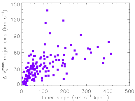
Figure 11: Mean rotation velocity difference $\Delta V_{c}^{mean}$ between actual $z=0$ and different $z=1.7$ rotation curves vs the actual $z=0$ rotation curve inner slope. Top: $\Delta V_{c}^{mean}$ is the mean difference between actual $z=0$ and non-corrected $z=1.7$ rotation curves. The $z=1.7$ rotation curves are computed along the major axis of the galaxies. Bottom: $\Delta V_{c}^{mean}$ is the mean difference between actual $z=0$ and model $z=1.7$ rotation curves. The $z=1.7$ rotation curves are computed using a “flat model”.

We also compared the inner slopes measured from $z=0$ rotation curves and from the model rotation curves. The scatter around $y=x$ line is very large, indicating that the use of such models to constrain mass modeling is not sufficient. AO observations are thus mandatory for mass modeling.

We find that galaxies with a beam smearing parameter $B^{>}_{\sim}3$ tend to present larger $\Delta V_{c}^{mean}$, but this trend is not very significant. This is due to the fact that large galaxies are also the fastest rotators and thus have larger inner slopes of the rotation curve. These large slopes are often explained by the presence of bulges and are well known in massive local galaxies dominated in their central region by the luminous matter distribution. However, without any high resolution broad band images, it is difficult to assess the presence of such bulges in high redshift galaxies. Furthermore, the rotation curve shape for high redshift galaxies is unknown and the presence of a bulge is not mandatory to observe a large inner velocity gradient.

On the other hand, rotation curves based on large clumps velocity measurements tend to underestimate the tangential velocity of the disk. These clumps have a radial velocity component which has to be taken into account (Bournaud, private communication). Thus, AO observations are needed to observed disk regions uncontaminated by the blurring of large clumps.

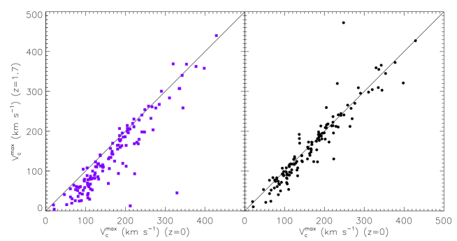
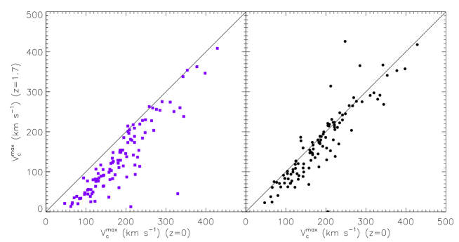
Figure 12: Comparison between the maximum rotation velocities at $z=0$ (x-axis) and $z=1.7$ (y-axis). The blue squares (left column) and the black dots (right column) represent respectively the maximum velocities measured along the major axis of the blurred velocity fields and the maximum deduced from the “flat model” fitting. (Top) Velocity fields are truncated at diameters $D_{25}$ (along the major axis). (Bottom) Velocity fields are truncated at diameters $D_{25}/2$.

We conclude that the distance effect is too important to recover a reliable rotation curve shape, in particular in the inner regions, whatever the beam smearing is up to at least $6$ (for larger values, our statistics are very poor), due to the sharper rotation curve shapes of large and massive galaxies. On the other hand, the unknown shape of high redshift rotation curves makes this comparison very approximative since if the slope is lower, the rotation curve shape should be better recovered.

6.4 Maximum rotation velocity analysis

Even without having a complete knowledge of the shape of a rotation curve, the first order analysis of kinematical data may allow a determination of the maximum rotation velocity of the rotation curve $V_{c}^{max}$. The latter is an important parameter to recover since it constrains the total amount of dynamical mass of the galaxies and is used for the analysis of the Tully-Fisher relation.

Two methods have been tested to retrieve this parameter. The first one consists in using the rotation curve computed along the major axis, which is equivalent to simulate a long slit aligned with the major axis, without taking beam smearing into account. With long slit spectroscopy, it is however possible to use models that take into account the seeing as done, e.g., by Weiner et al. (2006), but it is not straightforward to evaluate the contribution due to regions outside the slit. The second one consists in using the rotation curve models that account for the beam smearing. For both, $V_{c}^{max}$ is estimated from the maximum amplitude of the rotation curve within the extent of the velocity field along the major axis. In Figure 12, we compare the maximum rotation velocity determined by Epinat et al. (2008b) with those determined from these two methods. The model presented in this Figure is the “flat model”.

6.4.1 Major axis rotation curve

The maximum rotation velocity $V_{rc}^{max}$ directly determined from the rotation curve along the major axis without accounting for beam smearing is systematically underestimated for galaxies with rotation velocities lower than $\sim 150$ $km~{}s^{-1}$. The effect is even worse when we only consider the rotation curve limited to half the optical radius as it is shown on the Figure 12 (bottom). The maximum rotation velocity derived from rotation curve along the major axis (i.e. equivalent to rotation curves obtained using long slit spectroscopy instruments considering a good alignement with the actual position angle) is reliable for galaxies with an optical radius larger than three times the seeing ($B>3$), as seen in Figure 13 on which the relative difference between the maximum rotation velocities at $z=1.7$ and $z=0$ is plotted as a function of the beam smearing parameter $B$. The maximum rotation velocities determined from the rotation curve along the major axis are systematically underestimated by more than 25% for galaxies with $B$ lower than $2.5$. A correction to recover the actual maximum rotation velocity $V_{c}^{max}$ depending on the beam smearing parameter $B$ can be applied for smaller galaxies by making the assumption that the rotation curve shape is rather similar for high redshift and local galaxies:

$$V_{c}^{max}=\frac{V_{rc}^{max}}{0.1(\pm 0.2)+0.36~{}B}$$ (9)

The uncertainty given in parenthesis provides a range of corrections: the lower limit for the correction is given for $0.1+0.2$ and the upper limit for $0.1-0.2$.

This method may be improved in taking into account the beam smearing affecting the data along the major axis. Nevertheless, high redshift galaxies are strongly affected by the slit effect since they are poorly sampled due to their small angular size. Indeed, their angular size measured along the minor axis is comparable to the width of the long slit. In addition, the width of the long slit is usually larger than the seeing. Thus, without additional assumption on the spatial or spectral distribution, a confusion between the velocity and the position remains (slit effect). Moreover, flux distribution outside the slit is not constrained in long slit observations. Thus, assumptions on flux distribution are needed to take into account the contribution of external points to the velocity measurements.

6.4.2 Velocity field model

The model fitting enables to recover more reliable maximum rotation velocities even for slow rotators (Figure 12). The four rotation curve models have been compared. We find that the “flat model” statistically recovers better values than the other models (see Table 1). In particular, the three other models give very large maximum rotation velocities in a few case. In the case of exponential disk and isothermal halo models, this is due to the shape of these models that contains a central “bump”. In the case of the arctangent function, this is due to the fact that no plateau is reached unless the transition radius is very small (e.g. Appendix D). Due to the beam smearing, the models are mostly constrained by the inner regions that are more luminous. Indeed, one can observe the rather good agreement of the inner slope of the four models for all the rotation curves presented in Appendix D. The difficulty to recover the maximum rotation velocity for slow rotators is due to the fact that these galaxies are in addition intrinsically smaller, typically of the order of the beam size. The maximum rotation velocities derived from model fitting are statistically in good agreement with the actual maximum rotation velocities. This is especially convincing for the “flat model” (used in Figure 13) for which the determination is better than 25% even for galaxies with $B$ as low as $1$. The three other models may overestimate the maximum rotation velocities for some galaxies with $B$ smaller than $2$.

In conclusion, we have stressed that the use of integral field instruments sampling the seeing, enables a more robust modeling since off-axis points can be taken into account with less confusion than long slit spectrographs because they have an additional spatial dimension and allow to avoid slit effects. Moreover, we have shown that, using a simple flat rotation curve to model the disk, the maximum velocity can be recovered with an accuracy better than 25%, even for galaxies with a beam smearing parameter as low as 1.

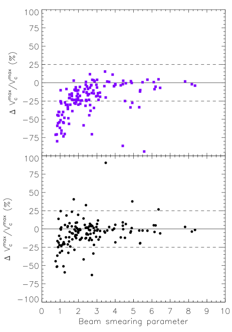
Figure 13: Relative difference between the maximum rotation velocities at $z=1.7$ and $z=0$ as a function of the beam smearing parameter $B$. The symbols are the same as in Figure 12.

6.5 Velocity dispersion analysis

6.5.1 Mean velocity dispersion and velocity shear

The local velocity dispersion $\sigma$ is a non trivial physical parameter to recover. Indeed, as explained in Appendix A, for each pixel, the measured velocity dispersion $\sigma_{1}$ is the quadratic combination of the local velocity dispersion plus a velocity shear feature induced by beam smearing effects. The velocity shear feature can however be extracted from the high resolution modeled velocity field if it correctly describes the observed velocity field. This requires a good estimate of the spatial PSF. Theoretically, as it is the case for the velocity field modeling, the velocity shear feature of the velocity dispersion map also needs the knowledge of a high spatial resolution line emission map.

The local velocity dispersion component is also affected by the low spatial resolution. Thus if we consider that the local velocity dispersion of the gas depends on the gravitational potential, we have to correct the velocity dispersion component from this effect. It is thus necessary to use a velocity dispersion model. In the present study, we avoid this by assuming that the local gas velocity dispersion is almost constant as observed in local galaxies (Epinat et al., in preparation). Thus, we measure the local velocity dispersion as the mean value of the velocity dispersion map quadratically corrected from the velocity shear term derived from the velocity field modeling (illustrated in Figure 14). Weiner et al. (2006) used both velocity and velocity dispersion to constrain their model, using a constant velocity dispersion model. This is an alternative approach from the method used in this paper. This has been discussed in section 5.

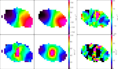
Figure 14: Example of comparison between high redshift simulated data (left column) and high redshift model mimicking the data (middle column) for the galaxy UGC 7901. A “flat model” has been used here. Top line: velocity field. Bottom line: velocity dispersion map. The difference between the simulated high redshift data (left columm) and the model (middle columm) is given for both the velocity field and the velocity dispersion map (quadratic difference) on the right column. The velocities are given by the rainbow scales on the right side of the images.

The velocity dispersion estimate also depends on the spectral resolution of the data. Our data that have a very high spectral resolution better than 10000 are probably not affected by spectral resolution effects. Spectral resolution effects will be studied in a forthcoming paper since we aim at probing spatial resolution effects only in the present study. Another difficulty with this parameter is its sensitivity to the signal-to-noise ratio that is usually low for high redshift observations. We do not consider this effect here since our data are not affected by a low signal-to-noise ratio. Moreover, if a constant local velocity dispersion model is assumed, all the points of the map should have the same velocity dispersion. There should be at least several points in the map with a sufficient signal-to-noise ratio in order to do an accurate measurement.

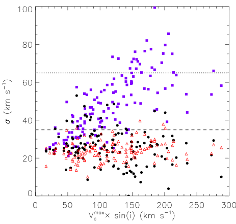
Figure 15: Velocity dispersion as a function of projected maximum velocity measured on $z=0$ velocity fields. Each point represents a galaxy. Blue squares correspond to the seeing-induced central velocity dispersion measured on $z=1.7$ maps (without applying any corrections). Red-open triangles represent the mean velocity dispersions measured on $z=0$ galaxies. The black dots correspond to the mean velocity dispersion measured on corrected velocity dispersion maps of $z=1.7$ galaxies using a “flat model”. The grey dashed and dotted lines respectively indicate the mean velocity dispersion in the IMAGES $z\sim 0.6$ sample and in a sample of forty-two $1<z<3$ objects observed with OSIRIS and SINFONI.

We conclude that a model is helpful to disentangle the velocity shear present in the velocity dispersion map from the local velocity dispersion. This is dramatically true for galaxies with a small beam smearing parameter.

6.5.2 Velocity dispersions vs rotation velocities

In Figure 15, the velocity dispersion is plotted as a function of the projected maximum velocity (observed at $z=0$) corrected for the inclination. Red-open triangles represent the velocity dispersion measurements for the local data. No dependency is observed with the projected maximum velocity. The local velocity dispersion does not depend either on the total radial velocity amplitude of the galaxy, suggesting that it does not depend on the galaxy mass. Blue squares represent seeing-induced velocity dispersions measured at the center of $z=1.7$ velocity dispersion maps and show a clear correlation with the projected maximum velocity. However, a large scatter is observed. This may be explained by the dependency of rotation curve shape with the true maximum velocity (Rubin et al., 1985; Persic et al., 1996; Catinella et al., 2006), in particular, the inner gradient is larger for fast rotators. These fast rotators observed with a low inclination should thus present a higher central velocity dispersion peak than slower rotators observed with a high inclination. This trend shows that the central velocity dispersion gives an indication about the shape of the inner rotation curve as well as the maximum velocity. The black dots represent the mean velocity dispersion measured on corrected velocity dispersion maps using a “flat model” being the one that statistically allows the best recovery of the local velocity dispersion (see Table 1). By comparing the error on the corrected velocity dispersion and the beam smearing parameter $B$ (not plotted), we note that the correction is statistically underestimated for galaxies with $B<2$, and often overestimated for other galaxies, probably due to both an insufficient resolution for the line flux maps and the rotation curve shape that rises rapidly for faster rotators. However, the correction is satisfactory since no strong correlation is seen anymore with the projected maximum velocity. Moreover, due to its low local velocity dispersion, the GHASP sample provides a strong constrain on the method. Indeed, the velocity shear contribution to the blurred velocity dispersion maps may be negligible for dispersion-dominated galaxies.

In conclusion, we have noticed that the mean gaseous local velocity dispersion does not depend on the mass for nearby galaxies contrarily to the projected sample. We have shown that the model we used for the projected galaxies is suitable to model high redshift kinematics. Indeed, it allows to remove the unresolved velocity shear contribution due to beam smearing and thus to recover the uniform velocity dispersion observed in nearby galaxies.

6.5.3 Velocity dispersion estimation used for the IMAGES sample

Flores et al. (2006) used the minimum observed value in the velocity dispersion maps in order to have an estimate of the local velocity dispersion. Indeed, it is necessary to discard from this measurement all the pixels affected by the velocity shear.

To test this method with our reference sample, the minimum velocity dispersion of the uncorrected and uncut velocity dispersion map has been compared to the mean velocity dispersion at $z=0$. We find that using such an estimate, the velocity dispersion is underestimated by a mean factor around $2$. We obtained a good agreement by estimating the velocity dispersion as the mean of the points with the 20% lowest velocity dispersion values on the redshifted velocity dispersion map, not limited to the optical radius. The comparison between this estimate and the mean velocity dispersion at $z=0$ is presented in Figure 16. Such an estimate has been motivated by the fact that $z=0$ velocity dispersion fluctuates from one region to another one. Moreover, the velocity dispersion is often slightly lower in the outer parts of galaxies (Epinat et al. in preparation), thus, the mean velocity dispersion at $z=0$ should be larger than the outer velocity dispersion. Such velocity dispersion measurements depend on the map extent, and thus on the signal-to-noise ratio of high redshift observations. This makes the estimator sensitive to this parameter in particular for rotation-dominated galaxies. Indeed, for dispersion-dominated galaxies, the local velocity dispersion may be easier to recover as the velocity shear is relatively less important. Note that this comparison with FLAMES/GIRAFFE data only indicates a trend since the sampling used in the present paper does not match the sampling of IMAGES dataset.

Figure 16: Minimum velocity dispersion of $z=1.7$ galaxies as a function of the mean velocity dispersion at $z=0$.

The conclusion is that this method allows to estimate the local velocity dispersion without the help of any model. However, it is very sensitive to both the signal-to-noise ratio and to the radial extent of the galaxy.

6.5.4 Unresolved beam and line-of-sight effects

The GHASP sample of local galaxies allows to test if high local velocity dispersions observed at high redshift may be the result of the integration, within a seeing disk, along the line-of-sight of individual HII regions.

From an observational point of view, in GHASP disks, the very central regions being excluded, the typical size of a bin for which the H$\alpha$ emission has a signal-to-noise ratio $\sim 7$ ranges from less than $0.1~{}kpc$ (one pixel) for the intense H$\alpha$ knots to $\sim 0.5~{}kpc$ for the most diffuse regions (Epinat et al., 2008b, c).

The local velocity dispersion within those bins (signal-to-noise ratio $\sim 7$) ranges from $10$ to $30$ $km~{}s^{-1}$. When these local galaxies are projected at high redshift, a seeing disk ($\sim 0.5$″) may thus contain more than $100$ bins, mixing along the line-of-sight the velocity components of several tens to several hundreds of individual regions. Taking into account the local velocity dispersion at $z=0$ and the number of regions integrated within a seeing disk at high redshift, even with the high spectral resolution of GHASP (which is not reached by far by any IFU spectrographs on 8-10 meter-class telescopes), the different components are undiscernible in the spectrum along the line-of-sight.

In conclusion, one has no way to know if the large local velocity dispersions seen in high redshift galaxies are due to very large, extended and massive clumps or, at the opposite, to the addition and the superposition along the line-of-sight within a seeing disk of a large amount of individual smaller clumps. This should be adressed using high resolution observations of the luminosity distribution (HST, AO or future JWST imaging).

6.5.5 Velocity dispersion evolution with the redshift

In order to study the evolution of the velocity dispersion with the redshift, we have compared the GHASP local sample with IMAGES sample (at $z\sim 0.6$) and with $z>1$ samples observed with SINFONI and OSIRIS. We have estimated the minimum value of the velocity dispersion map for each of the 63 galaxies of the IMAGES sample following Flores et al. (2006) and we have used the velocity dispersion values given by the authors for 42 $1<z<3$ galaxies observed with SINFONI (SINS and MASSIV pilot run) and OSIRIS.

At $z=0$, the GHASP sample used in this paper provides a mean local velocity dispersion of $24\pm 5$ $km~{}s^{-1}$. The mean local velocity dispersion for the whole IMAGES sample is $35\pm 18$ $km~{}s^{-1}$ while it reaches $\sim 65\pm 25$ $km~{}s^{-1}$ for $1<z<3$ galaxies (as illustrated by the dashed and dotted lines in Figure 15).

Moreover, it is interesting to notice that the mean local velocity dispersion in the IMAGES sample does not significantly differ for “rotating disk” ($37\pm 10$ $km~{}s^{-1}$), “perturbed rotation” ($34\pm 24$ $km~{}s^{-1}$) and “complex kinematics” ($35\pm 17$ $km~{}s^{-1}$). Using an alternative approach to compute the local velocity dispersion (excluding the central hot region and weighting by the signal-to-noise ratio after a 1-sigma bootstrapping), Puech et al. (2007) estimated slightly higher values ($\sim 45$ $km~{}s^{-1}$), but the previous conclusion does not change. This may indicate that different physical mechanisms (cosmological gas accretion, galaxy accretions, turbulence generated by self-gravity and/or star formation, etc.) may occur for galaxies having different histories and however lead to velocity dispersions having typically the same value. Alternatively, considering that a fraction of IMAGES “perturbed rotators” may be classified as “rotating disks” (see section 4), this could explain why no clear difference in the velocity dispersion is observed between both categories.

Contrarily to what is observed for nearby galaxies (see Figure 15), as already noticed in Epinat et al. (2009b), for $z>1$ galaxies, the maximum rotation velocities decreases when the local velocity dispersion increases (if we exclude the values from Law et al., 2009, since the latter are limited to the very inner part of the galaxies). Indeed, for the local GHASP sample, when no correction for beam smearing is applied, the velocity dispersion increases with the maximum rotation velocity. When the correction is applied, the velocity dispersion of these galaxies is not correlated to the maximum rotation velocity.

In conclusion, we note a clear and continuous increase of the local velocity dispersion with the redshift. This indicates an evolution of the galactic dynamics through the ages, from eleven Gyr ($z\sim 2.5$) to six Gyr ($z\sim 0.6$) up to now ($z\sim 0$). This might be due to the evolution of the dynamical support (dispersion towards rotation via e.g. violent relaxation processes) and/or to the evolution of non-circular motions (instabilities due to the presence of bars, etc.) and/or chaotic motions (turbulence, energy injection due to high star formation rates and/or AGNs).

6.6 Gravitational support

The ratio of the maximum circular rotation velocity $V_{c}^{max}$ and the local velocity dispersion $\sigma$ measures the nature of the gravitational support of a system in equilibrium. A high circular velocity compared to velocity dispersion ($V_{c}^{max}/\sigma>1$) is the signature of a rotation-dominated gravitational support, whereas a lower ratio ($V_{c}^{max}/\sigma<1$) is the signature of a dispersion-dominated system, as it is the case for elliptical galaxies. For nearby spirals, characteristic values for the local gaseous velocity dispersion $\sigma$ range from 10 to 40 $km~{}s^{-1}$ (see Figure 15).

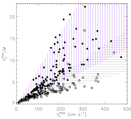
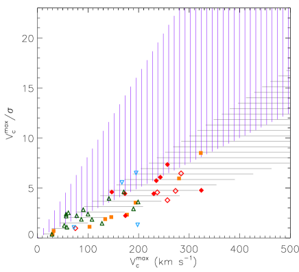
Figure 17: Ratio between the maximum rotation velocity and the mean velocity dispersion as a function of the maximum rotation velocity. Top. GHASP projected sub-sample. Circles: values uncorrected for the beam smearing. 85% of these circles are within the grey horizontal hatchings zone. Dots: values corrected for the beam smearing using the rotating disk modeling. 85% of these dots are within the purple vertical hatchings zone. The grey and purple hatchings are reported in the Bottom figure for reference. Bottom. Observed high redshift galaxies. Open symbols correspond to observations using AO. Red rhombuses: SINS rotating disks at $z\sim 2$ (Cresci et al., 2009). Orange squares: MASSIV pilot run galaxies at $z\sim 1.5$ (Epinat et al., 2009b). Green triangles: $z\sim 3$ Law et al. (2009) OSIRIS observations. Blue upside down triangles: rotating disks in Wright et al. (2007, 2009) at $z\sim 1.5$ observed with OSIRIS.

An interesting possible probe of the state of dynamical galaxy evolution is given by the behavior of this ratio $V_{c}^{max}/\sigma$ with the redshift. To test the beam smearing effects on the measure of the ratio $V_{c}^{max}/\sigma$, we have computed it for the projected GHASP sub-sample and compared it to actual distant galaxies. The ratio $V_{c}^{max}/\sigma$ as a function of $V_{c}^{max}$ has been plotted in Figure 17 for both local (top) and high redshift observed galaxies (bottom).

We have plotted GHASP local galaxies projected at $z=1.7$ using dots. These points have been computed using the maximum velocity $V_{c}^{max}$ derived from kinematics modeling and the velocity dispersion $\sigma$ corrected for beam smearing effects as explained in section 6.5. Since the GHASP sample is mainly composed of rotation-dominated galaxies, our sub-sample shows values of the ratio $V_{c}^{max}/\sigma$ lower than 2 only for very slow rotators ($V_{c}^{max}<100$ $km~{}s^{-1}$) and values ranging from $5$ to $20$ for rotators ranging from $100$ to $400$ $km~{}s^{-1}$. This ratio is strongly correlated with $V_{c}^{max}$ for local galaxies (slope $0.048~{}km^{-1}~{}s$), but with a large scatter. The correlation is expected since the velocity dispersion of the gas is rather constant with the maximum velocity for local galaxies, and the large scatter is due to the difficulty to recover both $V_{c}^{max}$ and $\sigma$ for the projected galaxies because of beam smearing effects. We have also plotted with circles the values without any correction for the beam smearing: the maximum velocity being computed from the rotation curve along the major axis and the velocity dispersion being estimated as the mean of the uncorrected velocity dispersion maps. The corresponding regions in which 85% of the points are lying have been reported on both plots of Figure 17 using vertical purple and grey horizontal hatchings. They respectively refer to beam smearing corrected and uncorrected points (see sections 6.4 and 6.5). Since the uncorrected maximum velocity and velocity dispersion are respectively underestimated and overestimated, grey and purple areas show only a small overlap. This grey area represents the “worst” estimation for the redshifted dataset.

From long slit spectrography, line-of-sight kinematic line widths ($\sigma$) of several hundreds good-quality measurements galaxies at $z\sim 1$, Weiner et al. (2006) roughly divided their sample into rotation ($V_{c}^{max}/\sigma>1$) and dispersion-dominated galaxies ($V_{c}^{max}/\sigma<1$). Dispersion-dominated galaxies are blue, mostly irregular and are not elliptical galaxies. These authors conclude that these galaxies probably have a disordered kinematics that is integrated over by the seeing.

Förster Schreiber et al. (2006) found that their three best rotators candidates at $z\sim 2$ show $V_{c}^{max}/\sigma\sim 2-4$, they concluded that these very gas rich disks are dynamically hot, geometrically thick and unstable to global star formation and fragmentation. These authors argue that these observations may be described by simulations (Immeli et al., 2004a) of gas-rich disks in which clumpy fragmentation disks are unstable and star forming clumps evolve by fuelling the galaxy center by dynamical friction and finally form a central bulge on $\sim 1$ Gyr time scale. Genzel et al. (2008) and Cresci et al. (2009) extended the SINS sample first described by Förster Schreiber et al. (2006) to 13 rotating disks candidates for which local velocity dispersion has been measured. They found $V_{c}^{max}/\sigma\sim 1-6$ with a mean value of 4.6.

Using 16 galaxies in the same range of redshift ($z\sim 2$), Law et al. (2009) found $V_{c}^{max}/\sigma\sim 0.1-1$ with a mean value of 0.5. These values are notably different from the SINS sample. As mentioned in section 3.2.9, the mean radius of the galaxies observed by Law et al. (2009) is eight times lower than for SINS galaxies. Moreover, their parameters (maximum velocity and velocity dispersion) are not corrected for the beam smearing and for inclination. Indeed, their maximum rotation velocity is the half of the whole shear whereas the velocity dispersion is flux-weighted, i.e. dominated by the inner regions. Similarly to Genzel et al. (2008), Law et al. (2009) concluded that the high velocity dispersion they observe may be neither a merger nor a disk, but rather the result of instabilities related to cold gas accretion.

In the redshift range of $1.2<z<1.7$, a compilation of 13 galaxies classified as rotators extracted from Wright et al. (2007), Wright et al. (2009) and Epinat et al. (2009b) provides $V_{c}^{max}/\sigma\sim 0.4-8.5$ with a mean value of 3.1. These values are comparable to the ones found at higher redshifts. Epinat et al. (2009b) argued that, considering the samples presently available, several processes may drive galaxy evolution. For instance, for their perturbed rotators, it is not straightforward to disentangle whether the high velocity dispersion is the result of gas accretion or gas rich minor mergers.

Bournaud et al. (2008) found $V_{c}^{max}/\sigma\sim 1-2$ (not corrected for inclination) for a clumpy galaxy at $z=1.6$ and proposed an internal fragmentation formation scenario of a gas-rich primordial disk becoming unstable. In comparing their SINFONI observations to numerical models, Bournaud et al. (2007) concluded that (i) complex morphology can result from the internal evolution of an unstable gas-rich disk galaxy and (ii) irregularities in the velocity field ($\sim$ several tens of $km~{}s^{-1}$) can be explained by clump-clump interactions that cause the individual velocity of each clump to differ significantly from the initial rotation velocity.

In Figure 17 (bottom), we have over-plotted the points corresponding to real high redshift galaxies. The values of these points have been corrected for beam smearing. Green triangles correspond to the galaxies observed by Law et al. (2007, 2009) at $z\sim 3$ with OSIRIS. These authors did not provide the inclination of the disks, thus we have used a mean statistic inclination of 45^∘ to compute the maximum rotation velocity in the galaxy plane. Moreover, we have corrected these velocities for beam smearing effect using the lower limit given in equation 9. This correction only provides lower values for $V_{c}^{max}$ since, due to the very small extent of these objects, the plateaus may not be reached. The local velocity dispersion has also been estimated from the velocity dispersion maps using the estimation given in section 6.5.3 instead of the flux-weighted velocity dispersion provided in Law et al. (2009) uncorrected for beam smearing effects. Blue upside down triangles are the rotating disks also observed with OSIRIS by Wright et al. (2007, 2009) at $z\sim 1.5$. Orange squares are galaxies part of MASSIV pilot run (Epinat et al., 2009b) and red rhombuses correspond to SINS rotating disks Cresci et al. (2009), both observed with SINFONI. Open symbols correspond to AO corrected observations. SINFONI setup in natural seeing observation has a pixel size of 0.125″ and a seeing around 0.5″. Observations using AO use a pixel size of 0.05″ with a seeing up to 0.2″. SINFONI spectral resolution is 4500 (70 $km~{}s^{-1}$) in K band, 3000 (100 $km~{}s^{-1}$) in H band and 1900 (160 $km~{}s^{-1}$) in J band. OSIRIS observations are using AO devices in order to have a seeing up to 0.1″ and use a pixel size of 0.05″ with a spectral resolution of 3600 (85 $km~{}s^{-1}$).

All these authors observed that, for a given circular velocity, $V_{c}^{max}/\sigma$ is lower for high redshift galaxies than for local galaxies. Several of them corrected for beam smearing but others did not. Since beam smearing artificially causes lower values of $V_{c}^{max}/\sigma$, the values for the projected sample obtained without correcting for the beam smearing effects provide a lower limit for nearby disks. Figure 17 shows that $V_{c}^{max}/\sigma$ values for high redshift galaxies, derived taking into account the seeing, are below this lower limit. This is thus a strong evidence for dynamical evolution between $z>1.5$ and $z\sim 0$.

We observe that the correlation for high redshift galaxies has a lower slope ($0.014~{}km^{-1}~{}s$) than for local galaxies, showing that high redshift galaxies are more dispersion-dominated. Ideally, to probe the gravitational potential, dispersion measurements should be done on the non collisional stellar component rather than on the collisional gas component. However, stellar kinematics are unreachable at high redshift with the current instrumentation. We could also notice that it is possible that the extent of high redshift galaxies may be lower than for low redshift galaxies and thus the maximum velocity may be missed. Another care is that it is probable that high redshift surveys have selection biases. Moreover, all these high redshift observations have a much lower spectral resolution than the local sample. We expect from this low spectral resolution that velocity dispersion correction is less accurate and thus that velocity dispersion measurements have much larger uncertainties.

6.7 Tully-Fisher relation

Table 2: Fits of local and distant Tully-Fisher relation.

Sample	Band	Slope $a~{}^{(a)}$	Zero point $b~{}^{(a)}$	Comment
GHASP local whole sample	B	$-7.2\pm 1.2$	$-3.97~{}^{(d)}$	Free slope, from Epinat et al. (2008b)
GHASP local sub-sample, RD$~{}^{(b)}$ $+$ PR$~{}^{(c)}$	B	$-6.2\pm 2.2$	$-6.23~{}^{(d)}$	Free slope
GHASP projected sub-sample, RD $+$ PR	B	$-5.2\pm 1.9$	$-8.68~{}^{(d)}$	Free slope
GHASP local sub-sample, RD	B	$-7.4\pm 1.7$	$-3.50~{}^{(d)}$	Free slope
GHASP projected sub-sample, RD	B	$-6.6\pm 1.4$	$-5.38~{}^{(d)}$	Free slope
GHASP projected sub-sample, RD	B	$-7.4$	$-3.67\pm 0.10$	Fixed slope
SDSS local subsample	K	$-6.88\pm 0.57$	$-6.54\pm 1.33$	Free slope, from Puech et al. (2008)
IMAGES $z\sim 0.6$, RD	K	$-7.24\pm 1.04$	$-5.07\pm 2.37$	Free slope, from Puech et al. (2008)
IMAGES $z\sim 0.6$, RD	K	$-6.88$	$-5.88\pm 0.09$	Fixed slope, from Puech et al. (2008)

(a): Tully-Fisher relation: $M=a\times\log{V_{c}^{max}}+b$. (b): RD refers to rotating disks. (c): PR to perturbed rotators. (d): Error bar on the zero point is not provided for the GHASP sample when the slope is free since it is very sensitive to changes in the slope. Keeping the slope fixed would lead to errors around $0.1$.

The Tully-Fisher relation is a way to constrain galaxy-formation models as well as to probe the dynamical stability of galaxies.

We computed the B-band Tully-Fisher relation for both local and redshifted GHASP sub-sample. As it has been done in Epinat et al. (2008b, c), the Tully-Fisher relation has been computed as the mean relation from the one obtained using a fit on absolute magnitudes as dependent variable and the one obtained using a fit on velocities as dependent variable. The errors are estimated as the difference between those two fits.

The GHASP sample is limited to rotating disks. It does not contain strongly interacting galaxies nor galaxies supported by random pressure. Nevertheless, as discussed in section 4, once projected and following the classification done by Flores et al. (2006), the kinematics of some galaxies may resemble to perturbed rotators. We first did not exclude any galaxy since we want to compare the scatter using the same projection parameters for both. Moreover, at high redshift, all the galaxies could be interpreted as rotating disks since they all present a velocity gradient at high redshift. Epinat et al. (2008b) found a slope of $-7.2\pm 1.2$ from the whole GHASP sample but excluding several galaxies because of their low inclinations (that induce strong uncertainties), or because their maximum velocity is probably not reached. From the local sub-sample defined in the present paper, the slope is estimated to $-6.2\pm 2.2$. This lower slope (although within the errors) can be explained by selection biases (see section 3.2.7): we only excluded the smallest galaxies, but not those that do not reach their maximum velocity or those with an inclination lower than $25$^∘. In particular, low mass galaxies hardly reach their maximum velocity within the optical radius, and Epinat et al. (2008b) have shown that the fastest rotators present a lower slope since they are less luminous than expected from local Tully-Fisher relation. The Tully-Fisher relation derived from the redshifted dataset is still lower ($-5.2\pm 1.9$) but compatible with the one derived from the local sub-sample within the error bars (see Table 2). This lower slope can be explained by beam smearing effects. Indeed, as shown in section 6.4, the maximum velocity is more difficult to recover for slow rotators than for fast rotators for which the model is better constrained. The scatter for those two slopes are rather similar and larger than the one derived by Epinat et al. (2008b), due to selection effects, in particular, the inclination inducing the strong scatter.

Absolute K-band magnitudes have been obtained for the IMAGES sample (Flores et al., 2006). Unfortunately, K-band photometry for the GHASP sample is not available, thus, we compare the B-band Tully-Fisher relation for the GHASP sample to the K-band Tully-Fisher relation for the IMAGES sample (Puech et al., 2008). This induces color-luminosity biases (e.g. Sakai et al., 2000; Verheijen, 2001). This data obtained with FLAMES/GIRAFFE instrument have a spectral resolution very similar to that of the GHASP redshifted data. Let’s notice however that GIRAFFE has a lower spatial resolution ($0.8$″ seeing and $0.52$″/pixel) than our simulations and a small spatial extent (6 by 4 spaxels).

Since a simple magnitude correction consists in adding a given value, the slopes should be comparable. Our slope is found to be lower than theirs (see Table 2). Their magnitude range however is tighter than ours as shown in Figure 2 and our sample thus contains lower luminosity systems for which the maximum velocity has not been derived with confidence. The slope determination is also highly dependent on the fitting method used. Surprisingly, assuming no evolution effects, we would have expected from IMAGES data a Tully-Fisher relation with a lower slope due to the instrumental spatial resolution differences between both samples. Indeed, the slope of the Tully-Fisher relation obtained from the projected GHASP sample is lower than the one obtained from high spatial resolution rotation curves (see Table 2). In addition, we have checked that this effect remains true whatever the magnitude range, in particular when the faintest galaxies are excluded.

In order to derive the Tully-Fisher relation in the same conditions as Puech et al. (2008), we also computed a Tully-Fisher relation using only galaxies that would be classified as “rotating disks”. Indeed, we noticed on the Tully-Fisher relation plots that some of the galaxies that Puech et al. (2008) classified as “complex kinematics” and “perturbed rotators” have their counterparts in our sub-sample, corresponding to galaxies that would be misclassified. By using “pertubed rotators” and “rotating disks” to derive their slope, they would probably have found a lower slope. Indeed, this is the trend that we observe when we use the whole GHASP sub-sample (see Table 2). In Figure 18 GHASP galaxies classified as “rotating disks” correspond to full points, and galaxies misclassified are displayed as open circles. The red continuous and black dashed lines correspond to the Tully-Fisher relation computed when using only galaxies that would be classified as “rotating disks” respectively for local and redshifted samples. These determinations are consistent with local determination: from the non redshifted sample we find a slope of $-7.4\pm 1.7$ and for the redshifted sample we find a slope of $-6.6\pm 1.4$ that is in agreement with the one derived at redshift $z\sim 0.6$ by (Puech et al., 2008). However, the trend is still to find a lower slope for the redshifted sample, although the difference is lower than the statistical error bars. The scatter also then becomes lower. Indeed, using only galaxies that would be classified as rotating disks imply that most of the low inclination systems are excluded as well as those with a solid body rotation curve for which the maximum is not determined with confidence. The use of the GHASP sample may indicate that the differentiation between “rotating disks” and “perturbed rotators” could be incorrect since GHASP galaxies misclassified as “perturbed rotators” are actually “rotating disks” and have the same behavior in our Tully-Fisher relation that in $z\sim 0.6$ relation. However, this classification enables in fact to exclude galaxies for which the lack of spatial resolution induces biases in the parameters determination.

Figure 18: Tully-Fisher relation at $z=0$ – red line – compared with Tully-Fisher relation computed at $z=1.7$ – black dots and black dashed line –. Open symbols correspond to galaxies that would not be classified as rotating disks at redshift 1.7. The two linear regressions (red line and black dotted line) are computed using only galaxies classified as rotating disks.

Since Puech et al. (2008) used K-band magnitudes, we cannot compare directly the Tully-Fisher zero point. However, the comparison between local and high redshift zero point can be probed. The Tully-Fisher zero point $b$ is defined by Puech et al. (2008) as

$$M=a\times\log{V_{c}^{max}}+b$$ (10)

In order to compare the zero point of their $z\sim 0.6$ sample and local value (from a SDSS sub-sample), they fixed the slope of the high redshift Tully-Fisher to the local slope. Thus, they found a galaxy brightening of $0.66\pm 0.14$ magnitude from $z\sim 0.6$ to $z=0$ that would indicate that galaxies double their stellar mass between these two epochs. They conclude that rotating disks observed at $z\sim 0.6$ should be rapidly transforming their gas into stars. We did the same comparison on our local and redshifted galaxies by fixing the slope to $-7.4$ found from the local galaxies classified as “rotating disks”. We found that beam smearing effects cannot account for the brightening suggested by Puech et al. (2008) since it leads to a difference of the zero point in Tully-Fisher relation equivalent to a loss of brightness of $0.17\pm 0.10$ magnitude. Considering that the uncertainty is of the same order of magnitude than the difference of zero point, we conclude that both local and redshifted zero points are compatible. This result would indicate that the signicative evolution of the Tully-Fisher zero point with respect to the error bars observed by Puech et al. (2008) is not accounted for by beam smearing effects.

In this section, we have discussed:

• The comparison between the local Tully-Fisher relation for the GHASP sample with the Tully-Fisher relation for the GHASP sample projected at high redshift. The conclusions are that the slope of the Tully-Fisher relation is lowered by beam smearing effects within the error bars and that the zero point of this relation is not significantly modified. This supports that the evolution of the zero point in the Tully-Fisher relation, observed by Puech et al. (2008), cannot be explained by beam smearing effects.
  
  

• The comparison between the slope of the Tully-Fisher relation for the GHASP sample projected at high redshift with the slope of the Tully-Fisher relation for the IMAGES sample. The conclusion is that the slopes of the Tully-Fisher relations derived from the GHASP sample projected at high redshift and from the IMAGES sample are compatible within the errors. Nevertheless, the latter comparison is limited (i) by the distributions in mass or in velocity of both samples that do not match, (ii) by the fact that the magnitude in the GHASP sample is computed in the B-band whereas it is computed in the K-band for the IMAGES sample and (iii) by the fitting methods used to compute the Tully-Fisher relation coefficients that are not exactly the same.

7 Discussion

A common explanation for massive galaxies having irregular kinematics and high nuclear gas fraction is that they may have undergone major mergers of gas-rich galaxies. On the other hand, models linking cosmological simulations to galaxy evolution (e.g. Ocvirk et al., 2008; Dekel et al., 2009) proposed a scenario where galaxies at $z\sim 2$ accrete significant amounts of cold gas which form unstable gaseous disks. Immeli et al. (2004a), followed by other authors, relaunched an old debate in suggesting that, in early-stage galactic disks, efficient gas cooling could have led to high cold gas fractions, which then fragmented due to self-gravity and collapsed to form a nuclear starburst. The kinematics of the brightest nebular emitting regions may be relatively featureless and may dominate the entire line emitting regions through the galaxy up to observable radii. The absence of shear may be a transient effect vanishing to further lower surface brightness ionized gas at later evolutionary stage.

7.1 Formation and evolution of high redshift gaseous disk

For rotating disks, at a resolution of a few kiloparsecs, it is challenging to know whether the large velocity dispersion observed in high redshift galaxies is due to (i) cold gas accretion, (ii) gas rich minor merger accretion events (e.g. Semelin & Combes, 2002) or (iii) wet major mergers. The three scenarios may fuel the disk in fresh gas. Scenario (i) might have two origins, internal or external to the galaxy. Indeed, huge reservoirs of gas, gravitationally bound to the galaxy (Pfenniger & Combes, 1994), may fuel the galaxies in cold gas as well as cold gas accretion flowing from the intergalactic medium. Both accretion mechanisms may lead to gas instabilities, cloud fragmentation and collapse, thus finally to strong starburst activity (Immeli et al., 2004b; Bournaud et al., 2008). The existence of a disk in rotation does not prove that it has been formed by continuous gas accretion. Indeed, if the initial spins of the progenitors are not too different, old wet major merger events may produce a rotating disk after a timescale $>0.5$ Gyr (shorter than the nowadays timescale) indistinguishable from a disk formed by the two other mecanisms. Alternatively, the presence of large reservoirs of gas around disk galaxies (Daddi et al., 2008) indicates that large amounts of gas are available to fuel the star formation. If minor mergers (10:1 to 50:1) occur with a high frequency, relaxation processes eject the pre-existing stars from the disk to the spheroid or to the thick disk. From an observal point of view, these stars are undistinguishable from the ones belonging to the thin disk. The formation of a spheroid or a thick disk will not perturb significantly the disk kinematics and its signature would be difficult to detect directly. Nevertheless, the stabilization of the disk due to these structures should be indirectly observable: they will diminish the star formation inducing less sub-structures as H$\alpha$ and UV clumps. A gaseous or stellar disk stable to all axisymmetric perturbations requires the Toomre’s parameters $Q>1$ (Safronov, 1960; Toomre, 1964). Giant star-forming clumps observed in high redshift galaxies, in which the star formation is as high as $100-1000M_{\odot}~{}yr^{-1}$, require high turbulent speeds and a dense disk with few stars in a spheroid (Bournaud & Elmegreen, 2009). The formation of these clumps requires that most of the stars and the gas lie in a rotating disk during the clump formation, otherwise $Q>1$, the disk is stable and massive clumps do not form. Indeed, halo as well as stellar speroid stabilize the disk and make the disk too stable to allow giant clumps to develop. The distribution, size and mass of these clumps may be considered as indirect indicators of the disk formation history. At the opposite, smooth diffuse gas accretion is not supposed to be efficient to form a stellar spheroid and instabilities dominate the disks and are observable through deep imaging addressing the formation of clumps. For very minors mergers (e.g. mass ratio $>$ 100:1), the dwarf galaxies are dislocated by the tidal field once they experience the gravitational field of the main galaxy. Torn by tidal field, this kind of accretion resembles very much to diffuse gas accretion. For a baryonic mass galaxy of $10^{10}M_{\odot}$, these satellites have masses lower than $10^{8}M_{\odot}$. If these galaxies exist, they are not detectable in observations or in numerical simulations, due to the lack of spatial resolution.

Large turbulence in the neutral gas disk could be provided by energy dissipation due to rapid external gas accretion (cosmological filaments, outer disk gas reservoirs). The huge sizes, masses and velocity dispersions of star-forming clumps still need to be understood. Taniguchi & Shioya (2001) favored a multiple merger origin similar to what is observed in several local compact groups. Noguchi (1999), Immeli et al. (2004a, b), Bournaud et al. (2007, 2008) proposed that, resulting from Jeans instabilities, primordial gaseous disk could fragment into several dense clumps. If the gas accretion is large and fast enough, the disk may become unstable leading to clumps formation with Jeans length-scale of $1-2$ kpc and Jeans mass-scale of $\sim 10^{8-9}M_{\odot}$. Unfortunately, the kpc-scale turbulence in the neutral atomic gas component (or the molecular gas via its CO content) has never been observed at high redshift. The presence of large clumps indicates nevertheless that it should be higher than in the local universe.

Disks observed at high redshift may be short-lived and not the precursors of today disk galaxies. Indeed, new pictures emerge in the literature in which young thick disks form by cold flows (Dekel et al., 2009; Kereš et al., 2009) and other types of diffuse gas accretion (Semelin & Combes, 2005), bulges form by internal and clump-driven evolution (Elmegreen et al., 2008; Genzel et al., 2008), and the thin disk forms later by further smooth accretion (e.g., Bournaud & Combes, 2002). Models discussed in Bournaud et al. (2007, 2008) predict that velocity shear tracing the initial gas rotation should be observed but with high velocity dispersion as shown by the observations of high redshift galaxies. In simulations including external gas accretion (Bournaud et al., 2008), the relatively thin initial disk ($700$ pc) becomes thicker ($\sim 1-2$ kpc). This is due to gravitational heating processes linked to clump formation processes. Stars formed in clumps constitute the thick disk or merge in the central bulge. The gas which has not been transformed in stars during the clump phase cools down and falls down in the pre-existing thin stellar disk.

The standard model indicates that massive galaxies formed earlier, thus having accreted their mass earlier and having been unstable at higher redshifts. As a consequence, their clumps should have been dispersed in the bulge or in the thick disk at earlier epochs than for less massive galaxies. Indeed, a bulge component seems to be already present in the most massive galaxies in the SINS sample.

7.2 What do observations of high redshift galaxies show?

7.2.1 Seeing-limited observations

Observations with a seeing disk of $\sim 4~{}kpc$ ($\sim 0.5$″) do not allow to sample the internal substructures of high redshift galaxies. Nevertheless, they are easier to obtain than AO ones. On the one hand, they do not require natural or laser guide star and, on the other hand, the larger pixel scale allow to observe the disk outskirts which have a lower surface brightness.

The bulk of SINS galaxies have been observed without AO (51 out of 63 galaxies) with a seeing disk of $\sim 0.6$″. Many SINS galaxies are bright and large, they have been selected from previous long slit observations (Erb et al., 2003, 2006) on the basis of consequent velocity shear and/or velocity dispersion. Among the 51 galaxies, 14 of them are classified as rotating disks (Cresci et al., 2009). These authors did not point out specific conclusions linked to the absence of AO and invoke the need for gas accretion to form disk as suggested by the predictions of the lastest N-body/hydrodynamical simulations of disk formation and evolution (e.g. Dekel et al., 2009).

In the frame of the MASSIV program, nine galaxies have been observed with a mean seeing of 0.65″ in the redshift range $1.2<z<1.6$ during a pilot run. Epinat et al. (2009b) found that six of them are compatible with rotators. They distinguished two rotating disks and four perturbed rotators showing a high velocity dispersion. For the MASSIV program, a special care is given in the selection of the targets. No definitive conclusion can yet be drawn. In particular for their perturbed rotators, they concluded that the high velocity dispersion may be the signature of gas accretion as well as gas rich minor mergers.

In conclusion, the SINS survey and the MASSIV pilot run reach roughly the same conclusion that almost a third of high redshift galaxies has rotation-dominated disks, another third has dispersion-dominated disks while the last third is composed of merging galaxy candidates. This is consistent with previous results obtained with long slit spectroscopy data by Weiner et al. (2006) and Kassin et al. (2007) who found one third of dispersion-dominated disks from more statistically complete samples. Forthcoming integral field spectroscopy data, like the MASSIV sample, will help in distinguishing between the various processes of galaxy formation acting at these redshifts. Indeed, the MASSIV sample has been selected from the VIMOS-VLT Deep Survey (Le Fèvre et al., 2005), which is both statistically representative of the overall population and volume complete, based on the measured masses and on-going star formation rate (Contini et al. et al., in preparation).

7.2.2 Adaptive optics observations

Adaptive optics observations allow to reach the kpc-scale which is a large improvement to analyze the internal kinematics of high redshift galaxies.

In the frame of the SINS program, twelve galaxies have been observed with SINFONI assisted by AO (Förster Schreiber et al., 2009). Only five of them, classified as rotating disks, have been published up to now (Genzel et al., 2008). The first observation by Genzel et al. (2006) of a high redshift galaxy (BzK 15504 at $z=2.38$) with an angular resolution of 150 mas ($\sim 1~{}kpc$) exhibits a resolved velocity shear which is nevertheless not well fitted by a simple disk model. With AO, the line-of-sight velocity dispersion remains high at high radii ($\sigma\sim 60-100$ $km~{}s^{-1}$) and the residual velocity map between the observed velocity field and the model (best-fitting exponential disk) shows deviations larger than 100 $km~{}s^{-1}$. Genzel et al. (2006) argued that it may be explained by radial gas inflows fuelling the central AGN.

The galaxy 1E0657-56 at $z=3.2$ being strongly lensed, SINFONI observations without AO of this object lead to a spatial resolution of $\sim 200~{}pc$ in the source plane, even better than AO resolution for non lensed galaxies. The position-velocity diagram within the central kpc of this galaxy looks like a rotating L_⋆ nearby spiral galaxy (Nesvadba et al., 2006) suggesting that, in some cases at least, a significant amount of mass could be already in place on small physical scale at $z\geq 3$.

OSIRIS instrument also assisted by AO has been used by Law et al. (2007, 2009) and Wright et al. (2007, 2009) for observing a total of 25 high redshift galaxies. Law et al. (2009) provide 16 galaxies at $z\sim 2-3$, including at most five rotating disks, resolved with a PSF $\sim 110-150$ mas. These authors concluded that, even for galaxies showing clear velocity gradients, rotation may not be the dominant mechanism of physical support. They refuted a simple bimodal disk/merger classifiaction scheme but underlined the dynamical importance of cold gas accretion. At lower redshifts ($\sim 1.5$), Wright et al. (2007, 2009) have observed nine galaxies, four of them have been classified as rotating disks. Among these four cases, two look like local disks while due to their high velocity dispersion, the two other ones look more like unstable disks.

7.2.3 High velocity dispersion in high redshift galaxies: comparison with local galaxies

We have shown in this work that, although the seeing-limited observations of intermediate and high redshift galaxies (from $z\sim 0.4$ to $z\sim 3$) suffer from significant beam smearing effects, it is not sufficient to explain the increase of velocity dispersion with the redshfift. Moreover, AO observations of high redshift galaxies reaching the lower limit of the kpc-scale also display a high velocity dispersion. This unambiguously indicates a clear and continuous dynamical evolution in disk galaxies through the last eleven Gyr. Three mechanisms act simultaneously and are responsible for gaseous velocity dispersion: turbulence due to local gravity, feedback linked to star formation processes and infall in the potential well of the galaxy. It is a challenging question to quantify the contribution of each processes.

Galaxies at earlier stages of evolution are observed to be very different from nowadays galaxies. Their high star formation rate of $\sim 10^{2-3}M_{\odot}$ per year has no equivalent in the local universe. This high star formation rate could be fuelled by large amounts of neutral and molecular gas. Theoretical calculations as well as observational evidence show that molecular cloud-cloud collision account for a substantial fraction of the star formation in the Galaxy (e.g. Tan, 2000, Sato et al., 2000 and references therein). In high redshift galaxies, high velocity dispersions up to $100$ $km~{}s^{-1}$ are observed in the warm phase of the gas on several kpc-scale, the velocity dispersion of the cold phase of the gas and of the stellar component being not observable. Very extended (as large as $\sim 1~{}kpc$) and massive star forming clumps ($\sim 10^{8-9}M_{\odot}$) are observed at redshift $\geq 1$, (e.g. Elmegreen et al., 2007 and references therein). Corresponding high-mass clumps do not exist in local galaxies, even in high star forming objects, where their masses do not exceed $\sim 10^{6}M_{\odot}$. On deca/hecto pc-scale, the typical velocity dispersion of the cold gas phase in the interstellar medium of local galaxies is of the order of $5$ $km~{}s^{-1}$: even in massive molecular clouds observed in local HII regions (e.g. $\sim 2.10^{5}M_{\odot}$ in NGC 7538, Minn & Greenberg, 1975), the internal velocity dispersion does not exceed $\sim 5$ $km~{}s^{-1}$. The formation of OB-stars associations leads to the ionization of smaller clumps, the so-called HII regions. Local gaseous velocity dispersion in nearby galaxies within HII regions spans only between 10 and 30  $km~{}s^{-1}$ (see section 6.5 and Weiner et al., 2006). During the strongest phase of star formation, mainly due to supernova activity, the ionized gas component is more turbulent and its velocity dispersion higher although not as high as observed in high redshift galaxies.

The mean rotation velocity of the ionized gas component may be similar to the unobserved neutral gas component (atomic or molecular). The spatial distribution of the ionized gas is more clumpy and its velocity dispersion higher than the neutral gas. It follows the distribution and dynamics of young stars and the stellar winds induced by them. Strong supernovae winds, large bubbles in expansion increase the velocity dispersion of the ionized gas and participate to the turbulent motions linked to star formation processes. However, turbulent motions observed through the ionized gas component, on kpc-scale structures, probably cannot be explained by star formation processes only. External mechanisms, like cosmological gas accretion, combined to local self-gravity are needed to provide additional energy to sustain the high velocity dispersions (Lehnert et al., 2009) and thus, should be present also in the neutral gas component. In nearby galaxies, a fraction of the local velocity dispersion observed in the gas is due to turbulence linked to mass density contrasts generated for instance by $m=2$ pertubations (spiral arms). At higher redshift, since gas density is higher, this turbulence linked to local gravity may increase and it will not indicate that the disk is unstable.

7.2.4 Large clumps observed in high redshift galaxies: huge HII regions or conglomerate of small clumps?

Galaxies are increasingly clumpy with redshift (Conselice et al., 2005). A large fraction of their luminous mass (up to 30%) and optical light (up to 50%) is confined to a few kpc-size clumps (Elmegreen & Elmegreen, 2005). These clumps are probably formed inside the galactic disk rather than entered from outside in a merger (Bournaud & Elmegreen, 2009). They are specific to high redshift galaxies that do not have spirals, nor bulges or exponential profiles. These clumps tell us about galaxy evolution and could be progenitors of modern spiral disks.

If these gaseous clumps are gravitationally bound and dynamically relaxed, they may trace the gravitational potential as it should be shown by the hidden stellar velocity dispersion. If one considers that the clumps observed at high redshift proceed from molecular clouds gravitationally bound as massive as $\sim 10^{9}M_{\odot}$, extrapolation of the scaling relation of Larson (1981) leads to internal velocity dispersion not higher that $\sim 25$ $km~{}s^{-1}$. To reach internal velocity dispersions $\sim 100$ $km~{}s^{-1}$, like those observed in clumps at high redshift, clump progenitors should have the mass of a massive galaxy ($\sim 10^{12}M_{\odot}$). These huge clumps may not be gravitationally linked systems or may be bound but not in equilibrium. The scaling relations of Larson (1981) are not valid to describe the physics of these clumps.

Many numerical works have been concerned with collision between so-called high-mass clouds which nevertheless do not excess $\sim 10^{3}M_{\odot}$ (e.g. Chapman et al., 1992). These clouds are obviously much less massive than the large clumps observed at high redshift. Nevertheless, one might expect a collision between two high-mass clouds to consist of many smaller-scale collisions between the clouds of lower mass of which the clumps are composed maybe down to $\sim 10~{}M_{\odot}$ (e.g. Kitsionas et al., 2008). These clumps may be the result of a high star-formation occurring at this stage but most massive clumps predicted in models simulating disk instability have a velocity dispersion $\sim 20-30$ $km~{}s^{-1}$ (Immeli et al., 2004a) or $40-50$ $km~{}s^{-1}$ (Bournaud et al., 2008). In other words, the mean local velocity scatter around circular motions (i.e. the dispersion in the rest frame of a disk in circular motion) expected from simulations ranges from $20$ to $50$ $km~{}s^{-1}$. The circular rotation of the clumps is given by the mean potential well of the galaxy (disk+dark halo) but clump-clump (2-body gravitational) interaction induces their velocity dispersion with an amplitude lower than $50$ $km~{}s^{-1}$. The high velocity dispersion observed on 2D velocity dispersion maps may be due to integration through the line-of-sight within the size of the unresolved observed beam. Very strong winds due to supernova activity may also increase the local velocity dispersion in the ionized gas component.

7.2.5 Large clumps at kpc-scale resolution

In this paper, we do not focus on merging systems but only on rotators for which three mechanisms of formation are possible: major mergers, minor mergers and gas accretion.

The assembly of galaxies at redshifts $z\sim 1-2$ which have clumps embedded in what appears to be a disk is unlikely to be mostly driven by hierarchical merging of smaller galaxies. Indeed, the formation of giant clumps (with the masses, sizes and elongations typically observed) in massive and highly turbulent disks, requires that the dominant process of mass assembly be some smooth accretion of cold and diffuse gas (Bournaud & Elmegreen, 2009). This is consistent with the picture in which young thick disks form by cold flows (Dekel et al., 2009; Kereš et al., 2009). However, the actual physical nature and the characterization of these clumps request further attention before disentangling different mechanisms occurring at different epoch of galaxy assembly.

The nature of the massive clumps observed in high redshift galaxies is well established from imaging (Conselice et al., 2005; Elmegreen & Elmegreen, 2005). Nevertheless, the lack of spatial resolution does not allow to fully characterize them. Indeed, large clumps with large velocity dispersions might be composed of several unresolved smaller clumps. Even if it is well established that the sizes, the luminosities, the velocity dispersion and thus the masses of these clumps are large with respect to the clumps observed in lower redshift galaxies, it may not be excluded that their “oversized” geometric and kinematics properties is due to the lack of resolution and to the fact that they are not resolved. In any cases, their physics is poorly understood and need higher spatial resolution to be modeled through numerical simulations. The high velocity dispersion in high redshift galaxies may be due to the blended kinematics of neighboring, self gravitating clouds. The low spatial resolution (limited by the seeing) combined with the low spectral resolution make difficult the deconvolution by both spatial and spectral instrumental PSF. Thus these large star forming clumps observed at high redshift maybe consist of the conglomerate of unresolved smaller scales clumps. In that case, the large velocity dispersion observed on kpc-scale in high redshift galaxies may thus be the result of the velocity dispersion of the different small clouds composing the unresolved clumps, rather than a local velocity dispersion within a large individual star-forming clump. Sub-kpc data are needed to observe sub-clumps in order to know if they are gravitationally bound or just spatial resolution effects.

Only high resolution observations may enable to compute velocity fields and rotation curves uncontaminated by the blurring of the data (see section 6.3). IFU AO observations provide in one shot a kpc-scale sampling both on the morphology and on the kinematics. These data are needed to sample the velocity field, rotation curve and velocity dispersion map, as discussed in section 6, and to recognize the disk formation mechanisms printed in the morphology and the kinematics.

8 Conclusion

Due to the lack of spatial resolution, consequence of their large distance, observations of galaxies at high redshift are affected by beam smearing effects. The different moment maps (intensity maps, velocity fields, velocity dispersion maps, etc.) as well as the one dimensional plots (line profiles, rotation curves, etc.) are severally blurred on kpc-scale. For instance, beam smearing effects completely modify the shape of the rotation curves in inducing artificially a solid body shape trend (i.e. a lower inner slope and a higher outer slope than real).

In this work, in order to study the biases induced by beam smearing effects existing in observation of high redshift galaxies and to provide new tools and recipes to analyse high redshift galaxies, we have used 3D data cubes for a large sample of local galaxies. This sample of nearby galaxies consists of 153 objects observed with Fabry-Perot technics belonging to the GHASP sample. We have simulated observations of this sample at redshift $1.7$ and have attempted to recover hidden information from the blurred velocity fields and velocity dispersion maps using simple kinematical models. The conclusions can be summarized through the different items as follows:

(I) The analysis led in this work enables us to test the validity of high redshift dynamical classification made by Flores et al. (2006); Yang et al. (2008) to distinguish rotating disks from mergers. We have shown that, using this classification, most of the rotating disks are correctly classified but we have also pointed out that around 30% of disk galaxies would be misclassified as perturbed rotators, or even complex kinematics. This may lower the fraction of galaxies with anomalous or perturbed kinematics in the IMAGES sample from 41% to 33%. This work will be further completed in projecting at high redshift a local sample of galaxies showing complex kinematics (mergers, close binaries, compact groups, blue compacts galaxies) in order to evaluate the fraction of these systems which would be misclassified as rotating disks.

(II) This sample was used to test the relevance of recovering the actual dynamical parameters of high redshift galaxies (inclination, position angle of the major axis, center, maximum rotation velocity, etc.) taking into account the lack of spatial resolution quantified by a “beam smearing parameter” $B$, ratio between the optical galactic radius ($D_{25}/2$) and the seeing FWHM. Actual observations generally lead to a $B$ parameter lower or equal to 2-3 without AO (e.g. Förster Schreiber et al., 2006) or even $B^{>}_{\sim}6$ when using AO (e.g. Genzel et al., 2008). The “recipes” to recover the dynamical parameters are the following:

• the position of the kinematical center is poorly constrained by the kinematics and should be fixed using high resolution broad-band images. When no clear center can be deduced from sub-kpc images of high redshift galaxies, as it is often the case, the position of the center is strongly affected by beam smearing effects. The determination of the center estimated by the symmetrization of the rotation curves is not reliable for galaxies showing a solid body shape at all radii, which is likely the case for galaxies with $B^{<}_{\sim}3$;

• the inclination needs to be constrained by high resolution morphologies since the agreement is better between high resolution morphological inclinations and high resolution kinematical inclinations than between high redshift and low redshift kinematical inclinations. The beam smearing however needs to be taken into account. In addition to the possible corrections already discussed in the literature (e.g. Simard et al., 2002; Peng et al., 2002), a simple way to do it consists in correcting half light radius major and minor axis by subtracting quadratically the seeing. The uncertainties in the determination of the kinematical inclination can be quantified by a linear function of the beam smearing parameter $B$;

• the position angle of the major axis is recovered with an accuracy better than 5^∘ for 70% of the sample using a 2D velocity field using simple rotating disk models, even with a rather low spatial resolution ($B\sim 2$);

• the observed velocity dispersion of the gas is strongly correlated with the velocity shear of the galaxy, especially in the inner regions. The local velocity dispersion $\sigma$ can be statistically recovered (i) by subtracting quadratically the velocity dispersion map model deduced from the velocity field modeling although with a large scatter or (ii) by considering regions with the lowest values that are the less affected by beam smearing. The larger the local velocity dispersion is, the weaker the above correlation is;

• the maximum velocity is statistically fairly well recovered for galaxies larger than three times the seeing in radius (i.e. with $B>3$), even if this limit probably depends on the unknown high redshift shape of the rotation curves. For galaxies with $B<3$, we provide a correction of the maximum velocity as a function of $B$. The use of a simple velocity field modeling enables to recover statistically the maximum velocity with an error lower than 25% in almost any case. We have also shown that a simple model of rotation curve consisting of a solid body part and a flat plateau statistically gives better estimates of the maximum velocity compared to exponential disk, isothermal sphere or arctangent rotation curve models;

• the local GHASP sub-sample of galaxies was also used to test different rotation curve models to recover the actual rotation curves, i.e. unaffected by beam smearing effects. A direct comparison between actual high resolution data ($z=0$) and various models was done in this purpose. In average, the various models are able to recover the general trend of the actual $z=0$ rotation curves but the scatter around the mean difference in the rotation curves ($\Delta V_{c}^{mean}$) is large, pointing out the difficulty to retrieve the actual shapes. Moreover, observations having a value of $B^{<}_{\sim}3$ do not allow suitable beam smearing corrections to recover the rough shape of the rotation curve whatever the model used. In order to be able to address problematics linked to the shape of the rotation curve (e.g. CORE vs CUSPY controversy about the inner density profile in spirals) for high redshift galaxies, $B^{>}_{\sim}10$ are necessary.

(III) Finally, this sample of local and evolved galaxies projected at high redshift has been compared to samples of actual high redshift galaxies observed using integral field capabilities (SINFONI, OSIRIS, GIRAFFE) to disentangle evolution effects from distance effects. By applying the same methods of analysis on both projected and observed samples, a relative comparison can be done to probe the kinematical evolution of galaxies, since the same observational biases exist in both samples. Our results suggest (i) that the trend in the evolution of the Tully-Fisher relation observed by Puech et al. (2008) is not due to beam smearing effects and (ii) that, except if no beam smearing correction is done on actual high redshift data, the high local velocity dispersion observed in high redshift galaxies cannot be reproduced in the local projected sample. This unambiguously means that, at the opposite of local evolved galaxies, it exists from redshifts $z\sim 3$ to $z\sim 1$ at least a population of disk galaxies for which a large fraction of the dynamical support is not only due to rotation but also to velocity dispersion. At $z\sim 0.6$, galaxies show intermediate velocity dispersions between local and higher redshift galaxies. This demonstrates a strong and continuous dynamical evolution in disk galaxies through the last eleven Gyr ($z\sim 2.5$). This conclusion is relevant at least for some galaxies among the relatively small sample of high redshift galaxies observed using IFU to date. Indeed, one cannot exclude important observation biases in the selection of the targets which was dictated by the feasibility of the observations rather than by strong considerations on the representativity of a given epoch by a set of galaxies correctly selected using for instance luminosity or mass functions. For a given observing time, multi-slit spectroscopy enables to observe larger samples than IFU techniques. However, due to the low spatial coverage per galaxy, long slit data does not allow a complete kinematical analysis.

The low numerical value for ($V_{c}^{max}/\sigma\sim 1-2$) is a convincing evidence for the existence of a population of thick and transient turbulent gas disks in high redshift galaxies. However, the large turbulence is a consequence of the large amount of gas which induces feedback, local gravitational disturbances and infall processes. It does not prove that the disk is formed by continuous gas accretion rather than by frequent wet minor mergers or old wet major mergers (Robertson & Bullock, 2008). If these thick disks are still seen later, they may be transformed into bulges and central galactic black hole. On the other hands, it has to be surveyed if the high redshift galaxies observed to date are representative of their epoch of formation or, alternatively, if the sample is biased by selection effects. These open questions justify the MASSIV on-going program (Contini et al. in preparation, Epinat et al., 2009b, Queyrel et al., 2009) dealing with galaxies ranging from $z\sim 1.0$ to $z\sim 1.8$ and selecting the targets using criteria making them representative of given epochs.

The spatial resolution reached by AO observations enables to reduce significantly the beam smearing effects. In this paper, the limits of the determination of kinematical parameters for high redshift galaxies observed under seeing limited conditions have been discussed: morphological and kinematical AO observations in the redshift range $0.5<z<3$ are essential to discuss the different scenarios of mass assambly and galaxy evolution.

In forthcoming works, the effects of spectral resolution and of the noise will be studied using the GHASP sample and local disturbed disk galaxies as compact groups galaxies (Torres et al. in preparation), blue compact star forming galaxies, strongly barred galaxies, mergers, close binaries will be compared to high redshift galaxies using the same methods presented in this paper.

The data used for this work will be available in a database under construction containing Fabry-Perot data http://fabryperot.oamp.fr/, enabling to retrieve directly from the database redshifted datacubes with a given seeing, pixel size and spectral resolution. This database will also contain data from several other Fabry-Perot surveys (barred galaxies; galaxies in clusters, in compact groups; blue compact galaxies, etc.).

Appendix A The model

A.1 Real light distribution

We note $S(x,y,\lambda)$ the spectral distribution of light at position $(x,y)$ at wavelength $\lambda$. This spectral distribution contains continuum ($C$) and line emission ($L$):

$$S(x,y,\lambda)=L(x,y,\lambda)+C(x,y)$$ (11)

The line flux or monochromatic flux is defined by equation 12:

$$M(x,y)=\int_{\lambda}L(x,y,\lambda)d\lambda$$ (12)

The velocity (first moment of the line) is defined by equation 13:

$$V(x,y)\equiv\overline{V(x,y)}=\frac{\int_{\lambda}L(x,y,\lambda)v(\lambda)d\lambda}{M(x,y)}$$ (13)

And finally, the local velocity dispersion (second moment of the line) is defined by equation 14:

$$\sigma(x,y)^{2}\equiv\overline{V(x,y)^{2}}-\overline{V(x,y)}^{2}$$ (14)

where

$$\overline{V(x,y)^{2}}=\frac{\int_{\lambda}L(x,y,\lambda)v(\lambda)^{2}d\lambda}{M(x,y)}$$ (15)

These are ideally the quantities that one wants to estimate. However this is not obvious as spectral PSF and spatial PSF are not Dirac distributions, and because instruments sample the light distributions through pixels and spectral channels.

A.2 Spectral PSF and sampling effects

The effect of the spectral PSF is a convolution with the spectrum:

$$S_{1}(x,y,\lambda)=L\otimes_{\lambda}PSF_{\lambda}+C$$ (16)

$PSF_{\lambda}$ being the spectral PSF. The spectral PSF can be considered constant within the wavelength range. Since the continuum does not vary with wavelength (by definition) it can be considered as null.

Spectral sampling is equivalent to convolving the spectrum with a “door” function:

$$S_{2}(x,y,\Lambda_{i})=\int_{\Lambda_{i}-\Delta\lambda/2}^{\Lambda_{i}+\Delta\lambda/2}S_{1}(x,y,\lambda)d\lambda$$ (17)

As spectral channels are contiguous, and because the spectral PSF does not introduce any loss in flux, the monochromatic flux can be expressed as:

$$M(x,y)=\sum_{i}S_{2}(x,y,\Lambda_{i})$$ (18)

By assuming that the rectangle method is giving a good estimate of integrals, that is true only when the spectral resolution (PSF and sampling) enables to oversample the line, the following equations can then be written:

$$\sum_{i}S_{2}(x,y,\Lambda_{i})v(\Lambda_{i})\approx\int_{\lambda}S(x,y,\lambda)v(\lambda)d\lambda$$ (19)

$$\sum_{i}S_{2}(x,y,\Lambda_{i})v(\Lambda_{i})^{2}\approx\int_{\lambda}S(x,y,\lambda)v(\lambda)^{2}d\lambda$$ (20)

This is the first approximation. It enables to deduce:

$$V(x,y)\equiv\overline{V(x,y)}=\frac{\sum_{i}S_{2}(x,y,\Lambda_{i})v(\Lambda_{i})}{M(x,y)}$$ (21)

$$\overline{V(x,y)^{2}}=\frac{\sum_{i}S_{2}(x,y,\Lambda_{i})v(\Lambda_{i})^{2}}{M(x,y)}$$ (22)

and then to express the velocity dispersion as in equation 14.

A.3 Spatial PSF and sampling effects

The spatial PSF, noted $PSF_{xy}$ is due to diffraction limit (Airy disk) as well as to seeing conditions. However, the induced defaults have to be compared with velocity variations.

A.3.1 Spatial PSF effects

The effect of the spatial PSF is a 2D convolution with the images:

$$S_{3}(x,y,\Lambda)=S_{2}(x,y,\Lambda)\otimes_{xy}PSF_{xy}$$ (23)

One can measure

$$M_{0}(x,y)=\sum_{i}S_{3}(x,y,\Lambda_{i})$$ (24)

And deduce from analytical computing that

$$M_{0}=M\otimes_{xy}PSF_{xy}$$ (25)

The measurement of the moments is also biased by this convolution :

$$\overline{V_{0}^{\alpha}}=\frac{\left[\overline{V^{\alpha}}M\right]\otimes_{xy}PSF_{xy}}{M_{0}}$$ (26)

By combining equation 14 and 26 we deduce the square of the blurred velocity dispersion before sampling:

$$\begin{split}\sigma_{0}^{2}=\frac{\left[\sigma^{2}M\right]\otimes_{xy}PSF_{xy}}{M_{0}}\\ +\frac{\left[\overline{V}^{2}M\right]\otimes_{xy}PSF_{xy}}{M_{0}}-\left(\frac{\left[\overline{V}M\right]\otimes_{xy}PSF_{xy}}{M_{0}}\right)^{2}\end{split}$$ (27)

A.3.2 Sampling effects

Spatial sampling is equivalent to convolve each frame with a 2D “door” function. Thus the measured spectrum is:

$$S_{4}(X,Y,\Lambda)=\int_{X-\Delta x/2}^{X+\Delta x/2}\int_{Y-\Delta y/2}^{Y+\Delta y/2}S_{3}(x,y,\Lambda)dxdy$$ (28)

To have lighter notations, the notation $\int_{pix}dxy$ is used instead of $\int_{X-\Delta x/2}^{X+\Delta x/2}\int_{Y-\Delta y/2}^{Y+\Delta y/2}dxdy$. The measured quantities are noted with the index $1$ ($M_{1}$, $V_{1}$, $\overline{V_{1}^{\alpha}}$, $\sigma_{1}$).

The observed flux is:

$$M_{1}(X,Y)=\sum_{i}S_{4}(X,Y,\Lambda_{i})$$ (29)

from which is deduced the link with the real monochromatic flux, by assuming that the spatial PSF does not depend neither on the wavelength nor on the position:

$$M_{1}(X,Y)=\int_{pix}M\otimes_{xy}PSF_{xy}dxy$$ (30)

In other words, the measured flux is the sum of the PSF convolved flux in one pixel. Within the same hypothesis, we deduce the observed momenta:

$$\overline{V_{1}^{\alpha}}(X,Y)=\frac{\int_{pix}\left[M\overline{V^{\alpha}}\right]\otimes_{xy}PSF_{xy}dxy}{M_{1}}$$ (31)

and thus, the expression of the observed velocity:

$$V_{1}(X,Y)\equiv\overline{V_{1}^{1}}(X,Y)=\frac{\int_{pix}\left[M\overline{V}\right]\otimes_{xy}PSF_{xy}dxy}{M_{1}}$$ (32)

and the square of the observed velocity dispersion:

$$\begin{split}\sigma_{1}^{2}(X,Y)\equiv\overline{V_{1}(X,Y)^{2}}-\overline{V_{1}(X,Y)}^{2}=\frac{\int_{pix}\left[\sigma^{2}M\right]\otimes_{xy}PSF_{xy}dxy}{M_{1}}\\ +\frac{\int_{pix}\left[\overline{V}^{2}M\right]\otimes_{xy}PSF_{xy}dxy}{M_{1}}-\left(\frac{\int_{pix}\left[\overline{V}M\right]\otimes_{xy}PSF_{xy}dxy}{M_{1}}\right)^{2}\end{split}$$ (33)

A.4 Comments

The previous set of equations is obtained with a very few hypothesis. It enables to understand why low resolution makes kinematical studies critical, in particular at high redshift. Moreover, it can be used as the basis to write kinematical models: it is possible to avoid the modeling of a data cube in order to gain computing time and resources. Modeling a velocity field is sufficient providing that we make some hypothesis on the flux distribution. Indeed, even if the flux distribution is known at the observing resolution, in the previous set of equations, we see the need for high resolution flux map. Ideally, high resolution narrow band observations should be provided to improve the modeling (using Tunable Filters for instance on space telescopes). HST data could also be used but making the approximation that the maps are tracing the gas distribution.

These equations also enable to disentangle resolution effects from real dispersion features in the velocity dispersion maps. Indeed, equation 33 presents a natural decomposition in two terms: a local velocity dispersion one and a velocity shear one due to the beam smearing. By using a satisfying velocity field model, unresolved velocity gradient can be subtracted quadratically from the velocity dispersion map. The remaining term is thus the local dispersion convolved with the spatial PSF. This term contains the signature of the spectral PSF. In particular, by making the hypothesis that the local velocity dispersion $\sigma$ is constant, what seems to be the case for the gaseous component for local galaxies, then the expression is simplified:

$$\begin{split}\sigma_{1}^{2}=\sigma^{2}+\frac{\int_{pix}\left[\overline{V}^{2}M\right]\otimes_{xy}PSF_{xy}dxy}{M_{1}}\\ -\left(\frac{\int_{pix}\left[\overline{V}M\right]\otimes_{xy}PSF_{xy}dxy}{M_{1}}\right)^{2}\end{split}$$ (34)

In the case one wants to constrain models with the velocity dispersion map, a velocity dispersion model has to be built.

A.5 Rotation curve models

Four models are used in this paper. These four models are only described with two parameters having the same physical signification: the maximum velocity $V_{t}$ of the function, and the radius at which it is reached $r_{t}$ (hereafter called transition radius) except for the arctangent model since the maximum velocity is reached at infinity. The transition radius is constrained to measure at least one pixel.

A.5.1 First model: exponential disk

This model describes a galaxy whose luminosity profile is fit with an exponential law, and for which the gravitation potential is uniquely due to the stars (no dark matter halo). It is a Freeman disk.

$$V(r)=\frac{r}{r_{0}}\sqrt{\pi G\Sigma_{0}r_{0}\left(I_{0}K_{0}-I_{1}K_{1}\right)}$$ (35)

Where $r_{0}$ is the exponential radius, $\Sigma_{0}$ is the central disk surface density, $I_{i}$ and $K_{i}$ are the i-order modified Bessel function evaluated at $0.5r/r_{0}$. The maximum velocity $V_{t}\sim 0.88\sqrt{\pi G\Sigma_{0}r_{0}}$ is reached at $r_{t}\sim 2.15r_{0}$. This model is the one used in Förster Schreiber et al. (2006).

A.5.2 Second model: isothermal sphere

This model describes the rotation curve due to an isothermal sphere dark matter halo. Spano et al. (2008) have shown that this model is the best fit model for local galaxies.

$$V(r)=\sqrt{4\pi G\rho_{0}r_{c}^{2}\left[\frac{r_{c}}{r}\ln\left(\frac{r}{r_{c}}+\sqrt{1+\frac{r^{2}}{r_{c}^{2}}}\right)-\frac{1}{\sqrt{1+\frac{r^{2}}{r_{c}^{2}}}}\right]}$$ (36)

Where $r_{c}$ is the core radius and $\rho_{0}$ is the central halo density. The maximum velocity $V_{t}\sim 0.54\sqrt{4\pi G\rho_{0}r_{c}^{2}}$ is reached at $r_{t}\sim 2.92r_{c}$. This model should be used when the contribution of the stars to the gravitation potential is negligible (i.e. for LSB galaxies).

A.5.3 Third model: “flat model”

This model does not describe any classical mass distribution. However, it can describe correctly lots of observed rotation curves of local galaxies, in particular those reaching a plateau.

$$V(r)=V_{t}\frac{r}{r_{t}}\mathrm{,for~{}}r<r_{t},$$ (37)

$$V(r)=V_{t}\mathrm{,for~{}}r\geq r_{t}.$$ (38)

This model is that used in Wright et al. (2007).

A.5.4 Fourth model: arctangent

This model is used by Puech et al. (2008). The rotation curve is described by an arctangent function. Since the maximum velocity is reached asymptotically for an infinite radius, the transition radius $r_{t}$ is defined as the radius for which the velocity reaches 70% of the asymptotic velocity $V_{t}$:

$$V(r)=V_{t}\frac{2}{\pi}\arctan{\frac{2r}{r_{t}}}$$ (39)

This function is rather similar to the “flat model” but is smoother. Moreover, the plateau is not clearly reached, thus it is more likely a rotation curve with an increasing plateau.

Appendix B Tables

Table 3: Galaxy parameters at $z=0$

Galaxy	$i_{z=0}~{}^{(a)}$	$PA_{z=0}~{}^{(b)}$	$D_{25}/2~{}^{(c)}$	$M_{B}~{}^{(d)}$	$V^{max}_{c}~{}^{(e)}$	$\sigma~{}^{(f)}$	$V^{max}_{c}/\sigma$	$S_{in}~{}^{(g)}$
	∘	∘	$kpc$	mag	$km~{}s^{-1}$	$km~{}s^{-1}$		$km~{}s^{-1}~{}kpc^{-1}$
UGC 89	$33\pm 13$	$177\pm 4$	$18.5$	$-21.5$	$343\pm 117$	$30\pm 17$	$11.4\pm 7.6$	$317\pm 26$
UGC 94	$42\pm 5$	$94\pm 2$	$17.2$	$-20.4$	$209\pm 21$	$23\pm 15$	$9.1\pm 6.0$	$118\pm 7$
UGC 508	$25\pm 7$	$123\pm 1$	$25.9$	$-21.8$	$553\pm 127$	$22\pm 16$	$25.1\pm 19.2$	$321\pm 24$
UGC 528	$21\pm 14$	$52\pm 3$	$3.5$	$-19.6$	$84\pm 52$	$24\pm 11$	$3.5\pm 2.7$	$103\pm 8$
UGC 763	$54\pm 6$	$117\pm 3$	$7.1$	$-18.9$	$104\pm 11$	$23\pm 13$	$4.5\pm 2.6$	$34\pm 2$
NGC 542	$90\pm 1$	$143\pm 9$	$9.9^{*}$	$-19.5$	$125\pm 8$	$28\pm 16$	$4.5\pm 2.6$	$-$
UGC 1249	$90\pm 1$	$150\pm 9$	$6.9$	$-18.3$	$65\pm 8$	$15\pm 15$	$4.3\pm 4.4$	$-$
UGC 1256	$76\pm 2$	$73\pm 2$	$7.2$	$-18.9$	$105\pm 9$	$17\pm 13$	$6.2\pm 4.8$	$29\pm 1$
UGC 1317	$73\pm 1$	$106\pm 1$	$26.0$	$-21.5$	$205\pm 9$	$27\pm 15$	$7.6\pm 4.2$	$110\pm 5$
UGC 1437	$47\pm 4$	$-53\pm 2$	$23.1$	$-21.8$	$218\pm 15$	$23\pm 18$	$9.5\pm 7.4$	$148\pm 10$
UGC 1655	$45\pm 18$	$-42\pm 6$	$29.0$	$-21.6$	$205\pm 64$	$16\pm 20$	$12.8\pm 16.5$	$195\pm 18$
UGC 1736	$35\pm 14$	$27\pm 2$	$11.3$	$-20.1$	$193\pm 68$	$19\pm 17$	$10.2\pm 9.8$	$50\pm 1$
UGC 1886	$62\pm 2$	$35\pm 1$	$34.0$	$-20.8$	$267\pm 8$	$19\pm 14$	$14.1\pm 10.4$	$27\pm 3$
UGC 2045	$61\pm 8$	$-41\pm 4$	$10.3$	$-20.5$	$137\pm 8$	$34\pm 11$	$4.0\pm 1.3$	$229\pm 15$
UGC 2082	$87\pm 4$	$133\pm 4$	$7.5$	$-18.3$	$100\pm 8$	$13\pm 14$	$7.7\pm 8.3$	$-$
UGC 2080	$25\pm 9$	$-24\pm 1$	$8.6$	$-19.2$	$131\pm 42$	$14\pm 13$	$9.4\pm 9.2$	$208\pm 16$
UGC 2141	$74\pm 23$	$-169\pm 4$	$4.2$	$-18.1$	$105\pm 8$	$30\pm 10$	$3.5\pm 1.2$	$36\pm 1$
UGC 2455	$51\pm 30$	$-97\pm 21$	$3.6$	$-18.6$	$21\pm 12$	$16\pm 14$	$1.3\pm 1.4$	$48\pm 4$
UGC 2800	$52\pm 13$	$-69\pm 3$	$6.5$	$-$	$103\pm 20$	$10\pm 13$	$10.3\pm 13.5$	$32\pm 1$
UGC 2855	$68\pm 2$	$100\pm 2$	$10.5$	$-21.4$	$229\pm 9$	$19\pm 15$	$12.1\pm 9.5$	$52\pm 1$
UGC 3013	$58\pm 8$	$-165\pm 3$	$22.8$	$-21.3$	$212\pm 21$	$29\pm 15$	$7.3\pm 3.8$	$203\pm 12$
UGC 3334	$47\pm 14$	$-83\pm 5$	$35.0$	$-22.8$	$377\pm 85$	$27\pm 16$	$14.0\pm 8.9$	$200\pm 7$
UGC 3382	$18\pm 6$	$-176\pm 2$	$9.9$	$-20.4$	$335\pm 111$	$17\pm 15$	$19.7\pm 18.6$	$58\pm 4$
UGC 3384	$45\pm 7$	$62\pm 59$	$4.1$	$-14.6$	$335\pm 111$	$21\pm 16$	$-$	$-$
UGC 3429	$54\pm 8$	$-43\pm 2$	$14.9$	$-21.3$	$248\pm 8$	$36\pm 14$	$6.9\pm 2.7$	$194\pm 6$
UGC 3463	$63\pm 3$	$110\pm 2$	$16.1$	$-20.7$	$168\pm 9$	$29\pm 14$	$5.8\pm 2.8$	$53\pm 3$
UGC 3574	$19\pm 10$	$99\pm 2$	$12.5$	$-18.0$	$202\pm 96$	$18\pm 14$	$11.2\pm 10.2$	$146\pm 7$
UGC 3521	$58\pm 5$	$-102\pm 2$	$9.7$	$-19.8$	$166\pm 12$	$21\pm 14$	$7.9\pm 5.3$	$46\pm 3$
UGC 3528	$42\pm 12$	$-137\pm 3$	$11.7$	$-20.1$	$276\pm 66$	$17\pm 14$	$16.2\pm 13.9$	$187\pm 11$
UGC 3691	$64\pm 4$	$-112\pm 2$	$8.7$	$-20.2$	$143\pm 10$	$29\pm 12$	$4.9\pm 2.1$	$84\pm 5$
UGC 3685	$12\pm 17$	$-62\pm 3$	$12.0$	$-19.7$	$133\pm 177$	$23\pm 13$	$5.8\pm 8.4$	$51\pm 1$
UGC 3708	$44\pm 16$	$-130\pm 4$	$8.0$	$-20.7$	$234\pm 69$	$40\pm 15$	$5.8\pm 2.8$	$132\pm 7$
UGC 3709	$55\pm 4$	$-128\pm 2$	$13.4$	$-21.5$	$241\pm 14$	$38\pm 16$	$6.3\pm 2.7$	$94\pm 6$
UGC 3734	$43\pm 7$	$139\pm 2$	$3.7$	$-18.6$	$108\pm 16$	$20\pm 14$	$5.4\pm 3.9$	$130\pm 3$
UGC 3809	$58\pm 2$	$-3\pm 1$	$32.1$	$-22.0$	$258\pm 9$	$16\pm 15$	$16.1\pm 15.1$	$65\pm 1$
UGC 3740	$48\pm 14$	$-113\pm 4$	$6.6$	$-19.8$	$87\pm 20$	$30\pm 10$	$2.9\pm 1.2$	$12\pm 2$
UGC 3851	$90\pm 1$	$30\pm 8$	$3.8$	$-17.1$	$65\pm 8$	$18\pm 12$	$3.6\pm 2.4$	$-$
UGC 3876	$59\pm 5$	$-2\pm 2$	$4.5$	$-17.4$	$112\pm 10$	$21\pm 15$	$5.3\pm 3.8$	$42\pm 3$
UGC 3915	$47\pm 4$	$30\pm 2$	$9.6$	$-21.4$	$205\pm 16$	$32\pm 14$	$6.4\pm 2.8$	$106\pm 6$
IC 476	$55\pm 24$	$68\pm 6$	$5.4^{*}$	$-19.0$	$70\pm 22$	$27\pm 14$	$2.6\pm 1.6$	$52\pm 4$
UGC 4165	$41\pm 10$	$-95\pm 2$	$4.4$	$-18.2$	$80\pm 18$	$22\pm 13$	$3.6\pm 2.3$	$71\pm 1$
UGC 4256	$38\pm 21$	$-69\pm 6$	$21.6$	$-21.6$	$123\pm 59$	$32\pm 18$	$3.8\pm 2.8$	$52\pm 4$
UGC 4273	$60\pm 4$	$-148\pm 2$	$11.4$	$-20.7$	$219\pm 11$	$21\pm 16$	$10.4\pm 8.0$	$172\pm 12$
UGC 4278	$90\pm 1$	$172\pm 4$	$6.2$	$-19.2$	$80\pm 8$	$20\pm 12$	$4.0\pm 2.4$	$-$
UGC 4284	$59\pm 9$	$176\pm 3$	$8.5$	$-18.4$	$118\pm 14$	$16\pm 12$	$7.4\pm 5.6$	$100\pm 4$
UGC 4325	$63\pm 14$	$57\pm 3$	$5.2$	$-18.2$	$85\pm 13$	$19\pm 13$	$4.5\pm 3.1$	$32\pm 1$
UGC 4393	$50\pm 9$	$-110\pm 7$	$9.7$	$-19.3$	$47\pm 10$	$28\pm 11$	$1.7\pm 0.7$	$8\pm 1$
UGC 4422	$25\pm 8$	$36\pm 1$	$25.3$	$-21.1$	$353\pm 94$	$23\pm 17$	$15.3\pm 12.1$	$308\pm 12$
UGC 4456	$9\pm 14$	$124\pm 3$	$18.5$	$-20.8$	$211\pm 321$	$25\pm 15$	$8.4\pm 13.8$	$111\pm 9$
UGC 4499	$50\pm 14$	$141\pm 3$	$4.4$	$-17.0$	$62\pm 13$	$20\pm 13$	$3.1\pm 2.1$	$22\pm 1$
UGC 4555	$38\pm 7$	$90\pm 2$	$12.7$	$-20.9$	$185\pm 30$	$24\pm 15$	$7.7\pm 5.0$	$111\pm 6$
UGC 4770	$20\pm 13$	$-82\pm 2$	$21.4$	$-21.3$	$330\pm 194$	$21\pm 17$	$15.7\pm 15.7$	$28\pm 3$
UGC 4820	$38\pm 3$	$157\pm 1$	$10.0$	$-20.3$	$336\pm 20$	$23\pm 14$	$14.6\pm 8.9$	$156\pm 13$
UGC 4936	$13\pm 12$	$-66\pm 2$	$22.2$	$-20.6$	$264\pm 227$	$20\pm 13$	$13.2\pm 14.2$	$59\pm 1$
UGC 5045	$16\pm 9$	$148\pm 2$	$17.4$	$-21.2$	$429\pm 228$	$28\pm 14$	$15.3\pm 11.2$	$95\pm 5$
UGC 5175	$56\pm 3$	$143\pm 1$	$11.0$	$-20.6$	$188\pm 10$	$34\pm 13$	$5.5\pm 2.1$	$71\pm 4$
UGC 5228	$72\pm 2$	$120\pm 1$	$8.3$	$-19.9$	$125\pm 9$	$27\pm 10$	$4.6\pm 1.7$	$57\pm 2$
UGC 5251	$73\pm 6$	$-100\pm 3$	$17.0$	$-20.5$	$125\pm 9$	$27\pm 11$	$4.6\pm 1.9$	$39\pm 1$
UGC 5253	$40\pm 4$	$-4\pm 1$	$13.3$	$-20.7$	$235\pm 17$	$21\pm 15$	$11.2\pm 8.0$	$254\pm 19$
UGC 5279	$90\pm 1$	$83\pm 7$	$7.9$	$-19.0$	$110\pm 8$	$26\pm 11$	$4.2\pm 1.8$	$-$
UGC 5316	$77\pm 4$	$130\pm 2$	$10.3$	$-19.9$	$145\pm 9$	$18\pm 15$	$8.1\pm 6.7$	$16\pm 1$
UGC 5319	$30\pm 9$	$-15\pm 1$	$8.2$	$-19.7$	$180\pm 47$	$25\pm 12$	$7.2\pm 3.9$	$73\pm 1$
UGC 5351	$82\pm 6$	$105\pm 7$	$6.5$	$-19.4$	$135\pm 8$	$32\pm 11$	$4.2\pm 1.5$	$-$
UGC 5414	$71\pm 13$	$-141\pm 4$	$4.6$	$-16.6$	$74\pm 10$	$20\pm 14$	$3.7\pm 2.6$	$26\pm 1$
IC 2542	$20\pm 15$	$174\pm 3$	$11.7^{*}$	$-20.5$	$290\pm 192$	$33\pm 15$	$8.8\pm 7.1$	$71\pm 1$
UGC 5510	$31\pm 10$	$-160\pm 2$	$7.7$	$-19.3$	$167\pm 44$	$26\pm 11$	$6.4\pm 3.2$	$134\pm 7$
UGC 5532	$32\pm 3$	$147\pm 1$	$22.0$	$-22.1$	$398\pm 24$	$27\pm 14$	$14.7\pm 7.7$	$382\pm 30$
UGC 5556	$75\pm 2$	$105\pm 8$	$9.0$	$-18.9$	$398\pm 24$	$27\pm 14$	$-$	$-$
UGC 5786	$53\pm 11$	$153\pm 5$	$6.0$	$-19.6$	$80\pm 15$	$36\pm 11$	$2.2\pm 0.8$	$294\pm 27$
UGC 5789	$68\pm 10$	$27\pm 3$	$12.0$	$-19.6$	$131\pm 10$	$20\pm 11$	$6.6\pm 3.6$	$12\pm 1$
UGC 5842	$47\pm 9$	$-68\pm 2$	$6.0$	$-18.8$	$115\pm 18$	$24\pm 15$	$4.8\pm 3.1$	$51\pm 1$
UGC 5931	$54\pm 16$	$0\pm 4$	$6.1$	$-19.8$	$157\pm 32$	$27\pm 13$	$5.8\pm 3.0$	$52\pm 3$
UGC 5982	$55\pm 4$	$28\pm 2$	$11.4$	$-20.0$	$199\pm 13$	$23\pm 14$	$8.7\pm 5.3$	$236\pm 19$
UGC 6118	$39\pm 8$	$-17\pm 3$	$7.3$	$-20.0$	$137\pm 24$	$31\pm 13$	$4.4\pm 2.0$	$403\pm 35$
UGC 6277	$17\pm 17$	$76\pm 3$	$9.3$	$-19.5$	$270\pm 258$	$24\pm 17$	$11.2\pm 13.4$	$274\pm 14$
UGC 6419	$66\pm 19$	$34\pm 6$	$5.3$	$-18.6$	$53\pm 11$	$26\pm 10$	$2.0\pm 0.9$	$5\pm 1$
UGC 6521	$46\pm 4$	$20\pm 2$	$19.2$	$-21.2$	$249\pm 18$	$26\pm 15$	$9.6\pm 5.6$	$64\pm 4$
UGC 6523	$24\pm 14$	$-7\pm 3$	$10.5$	$-21.0$	$118\pm 63$	$35\pm 13$	$3.4\pm 2.2$	$69\pm 5$
UGC 6537	$47\pm 5$	$-160\pm 2$	$12.1$	$-20.5$	$187\pm 17$	$18\pm 12$	$10.4\pm 7.0$	$25\pm 3$
UGC 6628	$20\pm 20$	$179\pm 2$	$6.1$	$-17.9$	$183\pm 168$	$17\pm 14$	$10.8\pm 13.3$	$60\pm 2$
UGC 6702	$38\pm 6$	$-104\pm 2$	$14.7$	$-20.6$	$195\pm 23$	$24\pm 15$	$8.1\pm 5.2$	$120\pm 11$
UGC 6778	$49\pm 4$	$-17\pm 1$	$9.5$	$-20.7$	$223\pm 14$	$25\pm 11$	$8.9\pm 4.0$	$352\pm 23$
UGC 7021	$56\pm 7$	$-94\pm 1$	$9.9$	$-19.7$	$223\pm 18$	$29\pm 14$	$7.7\pm 3.8$	$111\pm 6$
UGC 7045	$68\pm 2$	$99\pm 1$	$6.4$	$-19.2$	$160\pm 9$	$23\pm 11$	$7.0\pm 3.3$	$144\pm 4$
UGC 7154	$65\pm 3$	$-85\pm 1$	$13.1$	$-20.0$	$145\pm 9$	$23\pm 12$	$6.3\pm 3.3$	$124\pm 7$
UGC 7278	$44\pm 9$	$-20\pm 27$	$3.4$	$-17.4$	$145\pm 9$	$19\pm 11$	$-$	$-$
UGC 7323	$51\pm 11$	$38\pm 2$	$5.6$	$-18.3$	$84\pm 15$	$16\pm 13$	$5.2\pm 4.4$	$76\pm 4$
UGC 7699	$78\pm 2$	$32\pm 6$	$4.9$	$-17.6$	$92\pm 8$	$24\pm 11$	$3.8\pm 1.8$	$-$
UGC 7831	$56\pm 12$	$-70\pm 4$	$4.1$	$-18.5$	$92\pm 15$	$26\pm 9$	$3.5\pm 1.4$	$87\pm 2$
UGC 7853	$58\pm 28$	$-143\pm 3$	$5.1$	$-18.9$	$110\pm 35$	$24\pm 9$	$4.6\pm 2.3$	$20\pm 1$
UGC 7876	$53\pm 9$	$-16\pm 2$	$4.1$	$-17.9$	$98\pm 14$	$23\pm 11$	$4.3\pm 2.1$	$60\pm 1$
UGC 7901	$53\pm 2$	$-106\pm 1$	$11.3$	$-20.6$	$215\pm 10$	$25\pm 13$	$8.6\pm 4.5$	$191\pm 10$
UGC 7985	$49\pm 6$	$-84\pm 2$	$5.1$	$-18.7$	$112\pm 13$	$27\pm 10$	$4.1\pm 1.6$	$90\pm 1$
UGC 8403	$57\pm 4$	$121\pm 2$	$10.5$	$-19.2$	$128\pm 10$	$25\pm 10$	$5.1\pm 2.1$	$13\pm 1$
UGC 8490	$40\pm 15$	$167\pm 2$	$3.2$	$-17.1$	$90\pm 29$	$19\pm 13$	$4.7\pm 3.6$	$103\pm 4$
UGC 8709	$76\pm 1$	$-30\pm 1$	$27.1$	$-21.4$	$207\pm 9$	$27\pm 11$	$7.7\pm 3.1$	$32\pm 2$
UGC 8852	$52\pm 3$	$63\pm 1$	$8.8$	$-20.0$	$186\pm 10$	$25\pm 11$	$7.4\pm 3.3$	$84\pm 2$
UGC 8863	$77\pm 13$	$-142\pm 6$	$13.0$	$-20.3$	$191\pm 13$	$26\pm 13$	$7.3\pm 3.7$	$-$
UGC 8898	$27\pm 20$	$31\pm 6$	$11.7$	$-20.5$	$65\pm 45$	$23\pm 8$	$2.8\pm 2.2$	$65\pm 5$
UGC 8900	$57\pm 10$	$161\pm 2$	$19.5$	$-21.7$	$345\pm 37$	$25\pm 13$	$13.8\pm 7.3$	$62\pm 3$
UGC 8937	$32\pm 12$	$-175\pm 2$	$14.8$	$-21.1$	$320\pm 105$	$33\pm 15$	$9.7\pm 5.4$	$377\pm 34$
UGC 9013	$21\pm 16$	$164\pm 4$	$4.7$	$-18.2$	$62\pm 45$	$23\pm 10$	$2.7\pm 2.3$	$24\pm 1$
UGC 9179	$36\pm 14$	$49\pm 3$	$4.5$	$-17.8$	$111\pm 36$	$21\pm 11$	$5.3\pm 3.3$	$46\pm 3$
UGC 9219	$81\pm 6$	$99\pm 13$	$3.7$	$-16.6$	$45\pm 8$	$26\pm 13$	$1.7\pm 0.9$	$-$
UGC 9248	$58\pm 4$	$-99\pm 2$	$13.1$	$-20.2$	$166\pm 11$	$24\pm 15$	$6.9\pm 4.3$	$61\pm 1$
UGC 9358	$54\pm 4$	$-178\pm 2$	$13.3$	$-20.8$	$221\pm 14$	$29\pm 11$	$7.6\pm 2.9$	$245\pm 22$
UGC 9366	$62\pm 2$	$-135\pm 1$	$20.7$	$-21.7$	$241\pm 9$	$29\pm 14$	$8.3\pm 4.0$	$199\pm 13$
UGC 9363	$18\pm 14$	$147\pm 3$	$10.2$	$-19.8$	$143\pm 105$	$24\pm 11$	$6.0\pm 5.2$	$55\pm 2$
UGC 9406	$59\pm 25$	$132\pm 11$	$8.5$	$-19.0$	$19\pm 10$	$25\pm 12$	$0.8\pm 0.5$	$1\pm 1$
UGC 9465	$65\pm 4$	$127\pm 2$	$8.1$	$-18.0$	$97\pm 9$	$25\pm 10$	$3.9\pm 1.6$	$36\pm 1$
UGC 9576	$41\pm 11$	$122\pm 2$	$11.4$	$-19.6$	$104\pm 25$	$24\pm 11$	$4.3\pm 2.2$	$27\pm 2$
UGC 9649	$54\pm 6$	$-125\pm 2$	$3.9$	$-16.5$	$94\pm 11$	$19\pm 12$	$4.9\pm 3.2$	$191\pm 11$
UGC 9736	$51\pm 5$	$-141\pm 1$	$14.3$	$-20.6$	$192\pm 16$	$24\pm 14$	$8.0\pm 4.7$	$62\pm 4$
UGC 9753	$69\pm 1$	$3\pm 1$	$7.1$	$-19.1$	$138\pm 9$	$23\pm 13$	$6.0\pm 3.4$	$167\pm 4$
UGC 9858	$75\pm 2$	$70\pm 2$	$22.4$	$-20.4$	$160\pm 9$	$23\pm 15$	$7.0\pm 4.6$	$56\pm 1$
UGC 9943	$54\pm 2$	$-94\pm 1$	$11.1$	$-20.7$	$185\pm 10$	$26\pm 12$	$7.1\pm 3.3$	$167\pm 9$
UGC 9969	$61\pm 1$	$16\pm 1$	$27.2$	$-21.4$	$311\pm 9$	$22\pm 16$	$14.1\pm 10.3$	$61\pm 2$
UGC 10075	$62\pm 2$	$-150\pm 1$	$10.9$	$-19.9$	$168\pm 9$	$25\pm 10$	$6.7\pm 2.7$	$71\pm 2$
UGC 10310	$42\pm 20$	$-173\pm 6$	$4.9$	$-17.1$	$66\pm 27$	$22\pm 12$	$3.0\pm 2.0$	$20\pm 1$
UGC 10359	$44\pm 12$	$-76\pm 2$	$13.9$	$-19.0$	$143\pm 30$	$21\pm 14$	$6.8\pm 4.8$	$124\pm 7$
UGC 10470	$34\pm 9$	$-73\pm 2$	$8.8$	$-20.2$	$164\pm 39$	$27\pm 13$	$6.1\pm 3.3$	$106\pm 5$
UGC 10445	$47\pm 12$	$110\pm 4$	$6.4$	$-17.6$	$77\pm 17$	$23\pm 12$	$3.3\pm 1.9$	$36\pm 1$
UGC 10502	$50\pm 5$	$99\pm 2$	$19.8$	$-21.2$	$163\pm 14$	$19\pm 16$	$8.6\pm 7.3$	$27\pm 1$
UGC 10521	$59\pm 3$	$20\pm 2$	$7.3$	$-20.2$	$124\pm 9$	$27\pm 10$	$4.6\pm 1.7$	$53\pm 3$
UGC 10546	$42\pm 10$	$-178\pm 3$	$8.1$	$-19.1$	$106\pm 22$	$22\pm 14$	$4.8\pm 3.2$	$44\pm 3$
UGC 10564	$77\pm 6$	$149\pm 3$	$8.0$	$-17.6$	$75\pm 8$	$23\pm 12$	$3.3\pm 1.7$	$20\pm 1$
UGC 10713	$90\pm 1$	$8\pm 7$	$4.6$	$-19.0$	$105\pm 8$	$26\pm 11$	$4.0\pm 1.7$	$-$
UGC 10757	$44\pm 22$	$56\pm 5$	$3.9$	$-17.7$	$81\pm 33$	$28\pm 13$	$2.9\pm 1.8$	$90\pm 5$
UGC 10897	$31\pm 17$	$115\pm 3$	$7.1$	$-19.5$	$113\pm 56$	$18\pm 15$	$6.3\pm 6.1$	$41\pm 1$
UGC 11012	$72\pm 2$	$-61\pm 1$	$5.1$	$-18.7$	$117\pm 9$	$24\pm 10$	$4.9\pm 2.1$	$107\pm 3$
UGC 11124	$51\pm 10$	$-178\pm 3$	$8.2$	$-18.6$	$96\pm 15$	$22\pm 13$	$4.4\pm 2.7$	$33\pm 1$
UGC 11218	$58\pm 2$	$42\pm 1$	$11.9$	$-20.8$	$185\pm 9$	$22\pm 13$	$8.4\pm 5.0$	$105\pm 6$
UGC 11269	$69\pm 4$	$-88\pm 2$	$11.3$	$-19.9$	$202\pm 13$	$27\pm 14$	$7.5\pm 3.9$	$119\pm 11$
UGC 11283	$34\pm 17$	$120\pm 4$	$7.8$	$-19.3$	$173\pm 73$	$22\pm 14$	$7.9\pm 6.0$	$42\pm 4$
UGC 11283C	$68\pm 3$	$300\pm 15$	$4.0^{*}$	$-16.5$	$173\pm 73$	$17\pm 15$	$-$	$-$
UGC 11300	$70\pm 3$	$168\pm 2$	$4.4$	$-17.8$	$112\pm 9$	$17\pm 14$	$6.6\pm 5.5$	$161\pm 7$
UGC 11332	$82\pm 2$	$65\pm 5$	$8.3$	$-19.5$	$91\pm 8$	$29\pm 10$	$3.1\pm 1.1$	$-$
UGC 11407	$64\pm 22$	$65\pm 9$	$11.3$	$-20.8$	$158\pm 30$	$28\pm 12$	$5.6\pm 2.6$	$55\pm 3$
UGC 11429	$61\pm 16$	$-152\pm 5$	$20.1$	$-21.8$	$232\pm 35$	$20\pm 16$	$11.6\pm 9.4$	$35\pm 1$
UGC 11466	$66\pm 5$	$-134\pm 3$	$3.9$	$-18.5$	$133\pm 10$	$32\pm 12$	$4.2\pm 1.6$	$195\pm 6$
UGC 11496	$44\pm 16$	$167\pm 3$	$9.2$	$-$	$96\pm 29$	$24\pm 13$	$4.0\pm 2.5$	$18\pm 1$
UGC 11557	$29\pm 22$	$-84\pm 3$	$5.9$	$-18.4$	$105\pm 72$	$23\pm 13$	$4.6\pm 4.1$	$25\pm 1$
UGC 11707	$70\pm 4$	$59\pm 2$	$7.9$	$-16.6$	$97\pm 5$	$21\pm 13$	$4.6\pm 2.9$	$16\pm 1$
UGC 11852	$47\pm 7$	$-171\pm 2$	$15.9$	$-20.2$	$221\pm 27$	$25\pm 18$	$8.8\pm 6.5$	$41\pm 4$
UGC 11861	$43\pm 12$	$-142\pm 2$	$12.0$	$-20.2$	$181\pm 39$	$24\pm 15$	$7.5\pm 5.0$	$21\pm 1$
UGC 11872	$47\pm 3$	$86\pm 1$	$7.7$	$-20.0$	$183\pm 12$	$26\pm 14$	$7.0\pm 3.8$	$168\pm 9$
UGC 11909	$90\pm 1$	$1\pm 6$	$7.2$	$-19.3$	$110\pm 8$	$27\pm 12$	$4.1\pm 1.8$	$-$
UGC 11914	$33\pm 4$	$-94\pm 1$	$8.0$	$-20.3$	$285\pm 26$	$20\pm 15$	$14.2\pm 10.8$	$413\pm 31$
UGC 11951	$76\pm 8$	$-99\pm 4$	$4.6$	$-19.3$	$106\pm 7$	$25\pm 13$	$4.2\pm 2.2$	$32\pm 1$
UGC 12060	$36\pm 11$	$-173\pm 3$	$3.5$	$-16.5$	$107\pm 27$	$14\pm 15$	$7.6\pm 8.4$	$27\pm 2$
UGC 12276	$33\pm 15$	$-38\pm 5$	$15.1$	$-20.7$	$94\pm 37$	$22\pm 16$	$4.3\pm 3.5$	$19\pm 2$
UGC 12343	$52\pm 4$	$-157\pm 1$	$15.1$	$-21.1$	$221\pm 14$	$25\pm 14$	$8.8\pm 5.0$	$25\pm 1$
UGC 12754	$53\pm 5$	$-18\pm 2$	$5.3$	$-18.6$	$123\pm 11$	$15\pm 15$	$8.2\pm 8.2$	$237\pm 13$
(a): Inclination from Epinat et al. (2008b).
(b): Position angle of the major axis from Epinat et al. (2008b).
(c): Optical radius from the RC3 catalog (de Vaucouleurs et al., 1992) or from the HyperLeda database (refereed
by an asterisk ∗, Paturel et al., 2003).
(d): B-band magnitude from the HyperLeda database (Paturel et al., 2003).
(e): Maximum velocity from Epinat et al. (2008b).
(f): Mean local velocity dispersion.
(g): Inner slope of the rotation curve. No value is provided when no high resolution rotation curve is computed
(edge on galaxies, Epinat et al., 2008b, c).

Table 3: continued

Table 4: Exponential disk model on the sample projected at $z=1.7$

Galaxy$~{}^{(a)}$	$i_{z=1.7}~{}^{(b)}$	$PA_{z=1.7}~{}^{(c)}$	$r_{t}~{}^{(d)}$	$V_{t}~{}^{(e)}$	$V^{max}_{c}~{}^{(f)}$	$\sigma~{}^{(g)}$	$V^{max}_{c}/\sigma$	$\Delta V^{mean}_{c}~{}^{(h)}$	$S_{in}~{}^{(i)}$
	∘	∘	$kpc$	$km~{}s^{-1}$	$km~{}s^{-1}$	$km~{}s^{-1}$		$km~{}s^{-1}$	$km~{}s^{-1}~{}kpc^{-1}$
UGC 89	$10^{*}$	$169\pm 1$	$4.3\pm 0.1$	$401\pm 1$	$401$	$21\pm 20$	$19.4$	$-22$	$492$
UGC 94	$22\pm 1$	$91\pm 1$	$4.9\pm 0.1$	$232\pm 1$	$232$	$16\pm 15$	$14.5$	$-10$	$250$
UGC 508	$10^{*}$	$121\pm 1$	$10.2\pm 0.1$	$549\pm 1$	$549$	$27\pm 16$	$20.2$	$19$	$308$
UGC 528	$10^{*}$	$54\pm 3$	$\infty$	$\infty$	$44$	$35\pm 2$	$1.3$	$33$	$127^{*}$
UGC 763	$18\pm 9$	$119\pm 1$	$4.4\pm 0.1$	$103\pm 1$	$103$	$27\pm 5$	$3.8$	$-5$	$122$
NGC 542	$-$	$-$	$-$	$-$	$-$	$-$	$-$	$-$	$-$
UGC 1249	$-$	$-$	$-$	$-$	$-$	$-$	$-$	$-$	$-$
UGC 1256	$10^{*}$	$67\pm 1$	$7.3\pm 0.7$	$96\pm 2$	$96$	$25\pm 5$	$3.8$	$-4$	$73$
UGC 1317	$70\pm 1$	$103\pm 1$	$11.5\pm 0.1$	$229\pm 1$	$229$	$23\pm 15$	$9.8$	$1$	$115$
UGC 1437	$46\pm 1$	$-60\pm 1$	$8.7\pm 0.1$	$234\pm 1$	$234$	$29\pm 15$	$8.2$	$8$	$152$
UGC 1655	$10^{*}$	$-61\pm 1$	$1.1\pm 0.1$	$420\pm 1$	$420$	$0\pm 0$	$>100$	$-81$	$1628$
UGC 1736	$11\pm 10$	$28\pm 1$	$11.2\pm 0.2$	$194\pm 2$	$189$	$22\pm 13$	$8.6$	$-7$	$100$
UGC 1886	$63\pm 1$	$34\pm 1$	$13.1\pm 0.1$	$272\pm 1$	$272$	$16\pm 11$	$17.3$	$10$	$122$
UGC 2045	$10^{*}$	$-30\pm 1$	$12.5\pm 0.5$	$234\pm 5$	$167$	$31\pm 22$	$5.3$	$25$	$108$
UGC 2082	$-$	$-$	$-$	$-$	$-$	$-$	$-$	$-$	$-$
UGC 2080	$10^{*}$	$-23\pm 1$	$5.9\pm 0.1$	$130\pm 1$	$130$	$16\pm 6$	$8.3$	$-3$	$119$
UGC 2141	$80^{*}$	$-158\pm 3$	$\infty$	$\infty$	$71$	$41\pm 2$	$1.7$	$34$	$20^{*}$
UGC 2455	$10^{*}$	$-76\pm 8$	$\infty$	$\infty$	$10$	$24\pm 1$	$0.4$	$8$	$3^{*}$
UGC 2800	$43\pm 4$	$-75\pm 1$	$5.6\pm 0.3$	$94\pm 1$	$94$	$9\pm 9$	$10.6$	$-7$	$90$
UGC 2855	$37\pm 3$	$97\pm 1$	$11.3\pm 0.1$	$225\pm 1$	$225$	$19\pm 12$	$12.1$	$-5$	$115$
UGC 3013	$61\pm 35$	$-156\pm 1$	$\infty$	$\infty$	$502$	$26\pm 19$	$19.2$	$-19$	$24^{*}$
UGC 3334	$10^{*}$	$-83\pm 1$	$16.7\pm 0.1$	$400\pm 1$	$400$	$32\pm 19$	$12.7$	$19$	$143$
UGC 3382	$43\pm 1$	$-174\pm 1$	$10.5\pm 0.1$	$327\pm 2$	$327$	$14\pm 11$	$22.9$	$-4$	$179$
UGC 3384	$-$	$-$	$-$	$-$	$-$	$-$	$-$	$-$	$-$
UGC 3429	$10^{*}$	$-34\pm 1$	$12.7\pm 0.8$	$319\pm 11$	$301$	$44\pm 30$	$6.8$	$31$	$146$
UGC 3463	$62\pm 1$	$108\pm 1$	$10.3\pm 0.1$	$176\pm 1$	$176$	$32\pm 9$	$5.5$	$-3$	$98$
UGC 3574	$48\pm 1$	$102\pm 1$	$10.3\pm 0.2$	$192\pm 1$	$192$	$20\pm 6$	$9.5$	$5$	$107$
UGC 3521	$53\pm 1$	$-105\pm 1$	$6.7\pm 0.1$	$162\pm 1$	$162$	$13\pm 13$	$12.5$	$-7$	$133$
UGC 3528	$51\pm 1$	$-134\pm 1$	$2.7\pm 0.1$	$302\pm 1$	$302$	$13\pm 18$	$22.7$	$-36$	$558$
UGC 3691	$68\pm 2$	$-114\pm 1$	$46.5\pm 4.4$	$283\pm 19$	$147$	$34\pm 9$	$4.4$	$9$	$39$
UGC 3685	$10^{*}$	$-67\pm 1$	$5.5\pm 0.2$	$92\pm 1$	$92$	$24\pm 4$	$3.8$	$8$	$90$
UGC 3708	$10^{*}$	$-119\pm 1$	$1.1\pm 0.1$	$291\pm 1$	$291$	$15\pm 22$	$19.8$	$-80$	$1161$
UGC 3709	$55\pm 1$	$-132\pm 1$	$9.2\pm 0.1$	$257\pm 1$	$257$	$36\pm 19$	$7.1$	$-11$	$157$
UGC 3734	$10^{*}$	$136\pm 1$	$1.1\pm 0.1$	$124\pm 1$	$124$	$6\pm 7$	$19.3$	$3$	$498$
UGC 3809	$60\pm 1$	$-3\pm 1$	$11.9\pm 0.1$	$271\pm 1$	$271$	$20\pm 15$	$13.2$	$-10$	$132$
UGC 3740	$54\pm 3$	$-113\pm 1$	$9.3\pm 0.9$	$75\pm 3$	$72$	$37\pm 2$	$2.0$	$11$	$46$
UGC 3851	$-$	$-$	$-$	$-$	$-$	$-$	$-$	$-$	$-$
UGC 3876	$61\pm 6$	$5\pm 1$	$4.5\pm 0.5$	$115\pm 2$	$115$	$32\pm 8$	$3.6$	$-9$	$135$
UGC 3915	$39\pm 1$	$30\pm 1$	$4.1\pm 0.1$	$225\pm 1$	$225$	$28\pm 16$	$8.2$	$-7$	$288$
IC 476	$80^{*}$	$64\pm 1$	$\infty$	$\infty$	$84$	$25\pm 12$	$3.3$	$20$	$29^{*}$
UGC 4165	$10^{*}$	$-99\pm 1$	$2.1\pm 0.3$	$88\pm 3$	$88$	$22\pm 7$	$4.0$	$-9$	$202$
UGC 4256	$70\pm 1$	$-65\pm 1$	$21.1\pm 0.4$	$124\pm 2$	$123$	$47\pm 8$	$2.6$	$44$	$36$
UGC 4273	$53\pm 1$	$-149\pm 1$	$10.2\pm 0.1$	$190\pm 1$	$190$	$27\pm 10$	$6.9$	$18$	$106$
UGC 4278	$-$	$-$	$-$	$-$	$-$	$-$	$-$	$-$	$-$
UGC 4284	$67\pm 1$	$176\pm 1$	$18.8\pm 1.0$	$158\pm 5$	$110$	$20\pm 10$	$5.5$	$7$	$51$
UGC 4325	$11\pm 35$	$57\pm 1$	$1.1\pm 0.1$	$104\pm 1$	$104$	$14\pm 10$	$7.3$	$-24$	$428$
UGC 4393	$10^{*}$	$-110\pm 1$	$\infty$	$\infty$	$58$	$31\pm 5$	$1.9$	$-4$	$6^{*}$
UGC 4422	$20\pm 1$	$35\pm 1$	$9.8\pm 0.1$	$364\pm 1$	$364$	$25\pm 15$	$14.4$	$44$	$211$
UGC 4456	$14\pm 4$	$124\pm 1$	$14.9\pm 0.2$	$184\pm 1$	$184$	$25\pm 5$	$7.3$	$32$	$73$
UGC 4499	$10^{*}$	$145\pm 1$	$1.1\pm 0.1$	$110\pm 1$	$110$	$4\pm 7$	$26.2$	$-56$	$448$
UGC 4555	$44\pm 1$	$91\pm 1$	$8.6\pm 0.1$	$187\pm 1$	$187$	$19\pm 11$	$9.7$	$5$	$122$
UGC 4770	$10^{*}$	$-79\pm 1$	$26.5\pm 0.3$	$397\pm 2$	$378$	$25\pm 13$	$15.2$	$-29$	$93$
UGC 4820	$10^{*}$	$156\pm 1$	$1.9\pm 0.1$	$458\pm 2$	$458$	$1\pm 3$	$>100$	$-71$	$1123$
UGC 4936	$18\pm 2$	$-66\pm 1$	$11.1\pm 0.1$	$226\pm 1$	$226$	$22\pm 6$	$10.5$	$-4$	$117$
UGC 5045	$10^{*}$	$146\pm 1$	$10.1\pm 0.1$	$447\pm 1$	$447$	$30\pm 9$	$14.8$	$-8$	$252$
UGC 5175	$48\pm 1$	$143\pm 1$	$6.3\pm 0.1$	$199\pm 1$	$199$	$26\pm 9$	$7.5$	$-11$	$173$
UGC 5228	$10^{*}$	$119\pm 1$	$5.1\pm 0.1$	$143\pm 1$	$143$	$24\pm 14$	$6.0$	$-15$	$150$
UGC 5251	$63\pm 2$	$-102\pm 1$	$11.9\pm 0.1$	$136\pm 1$	$136$	$24\pm 11$	$5.7$	$-9$	$66$
UGC 5253	$45\pm 1$	$-5\pm 1$	$3.6\pm 0.1$	$266\pm 1$	$266$	$10\pm 13$	$27.1$	$-5$	$382$
UGC 5279	$-$	$-$	$-$	$-$	$-$	$-$	$-$	$-$	$-$
UGC 5316	$10^{*}$	$127\pm 1$	$26.7\pm 1.3$	$167\pm 5$	$131$	$20\pm 7$	$6.5$	$-9$	$39$
UGC 5319	$31\pm 2$	$-11\pm 1$	$7.7\pm 0.2$	$181\pm 1$	$181$	$28\pm 7$	$6.4$	$4$	$131$
UGC 5351	$-$	$-$	$-$	$-$	$-$	$-$	$-$	$-$	$-$
UGC 5414	$10^{*}$	$-151\pm 3$	$\infty$	$\infty$	$56$	$32\pm 2$	$1.8$	$10$	$24^{*}$
IC 2542	$34\pm 1$	$174\pm 1$	$7.1\pm 0.1$	$304\pm 1$	$304$	$33\pm 12$	$9.3$	$-17$	$236$
UGC 5510	$10^{*}$	$-161\pm 1$	$9.2\pm 0.3$	$166\pm 2$	$164$	$33\pm 5$	$5.0$	$20$	$103$
UGC 5532	$30\pm 1$	$147\pm 1$	$6.5\pm 0.1$	$381\pm 1$	$381$	$29\pm 13$	$13.2$	$29$	$319$
UGC 5556	$-$	$-$	$-$	$-$	$-$	$-$	$-$	$-$	$-$
UGC 5786	$80^{*}$	$154\pm 1$	$\infty$	$\infty$	$83$	$53\pm 4$	$1.6$	$39$	$16^{*}$
UGC 5789	$59\pm 2$	$31\pm 1$	$20.0\pm 0.6$	$123\pm 2$	$114$	$17\pm 9$	$6.8$	$-2$	$37$
UGC 5842	$70\pm 3$	$-68\pm 1$	$52.3\pm 17.0$	$330\pm 82$	$118$	$32\pm 7$	$3.7$	$13$	$41$
UGC 5931	$10^{*}$	$9\pm 1$	$\infty$	$\infty$	$128$	$37\pm 6$	$3.4$	$28$	$27^{*}$
UGC 5982	$49\pm 1$	$31\pm 1$	$6.6\pm 0.1$	$202\pm 1$	$202$	$12\pm 13$	$16.4$	$4$	$168$
UGC 6118	$80^{*}$	$-25\pm 1$	$\infty$	$\infty$	$191$	$42\pm 20$	$4.6$	$39$	$33^{*}$
UGC 6277	$10^{*}$	$76\pm 1$	$6.6\pm 0.4$	$243\pm 5$	$236$	$42\pm 8$	$5.6$	$26$	$202$
UGC 6419	$10^{*}$	$40\pm 3$	$1.4\pm 0.7$	$30\pm 7$	$30$	$27\pm 1$	$1.1$	$2$	$94$
UGC 6521	$47\pm 1$	$20\pm 1$	$8.6\pm 0.1$	$256\pm 1$	$256$	$27\pm 14$	$9.4$	$6$	$167$
UGC 6523	$10^{*}$	$-6\pm 1$	$2.4\pm 0.1$	$115\pm 1$	$115$	$39\pm 8$	$2.9$	$-8$	$235$
UGC 6537	$27\pm 1$	$-164\pm 1$	$4.6\pm 0.1$	$188\pm 1$	$188$	$10\pm 10$	$18.3$	$-18$	$217$
UGC 6628	$42\pm 7$	$-179\pm 1$	$8.4\pm 1.1$	$142\pm 8$	$138$	$23\pm 7$	$6.0$	$0$	$95$
UGC 6702	$45\pm 1$	$-107\pm 1$	$5.5\pm 0.1$	$215\pm 1$	$215$	$16\pm 14$	$13.5$	$20$	$210$
UGC 6778	$28\pm 2$	$-18\pm 1$	$7.9\pm 0.1$	$204\pm 1$	$204$	$29\pm 12$	$7.0$	$19$	$145$
UGC 7021	$27\pm 3$	$-105\pm 1$	$6.1\pm 0.2$	$140\pm 1$	$140$	$45\pm 12$	$3.1$	$69$	$124$
UGC 7045	$34\pm 12$	$100\pm 1$	$4.9\pm 0.1$	$178\pm 1$	$178$	$11\pm 12$	$16.1$	$-15$	$191$
UGC 7154	$62\pm 1$	$-84\pm 1$	$15.7\pm 0.2$	$135\pm 1$	$133$	$24\pm 7$	$5.6$	$2$	$51$
UGC 7278	$-$	$-$	$-$	$-$	$-$	$-$	$-$	$-$	$-$
UGC 7323	$10^{*}$	$35\pm 1$	$5.0\pm 0.5$	$77\pm 2$	$77$	$24\pm 5$	$3.2$	$-3$	$82$
UGC 7699	$-$	$-$	$-$	$-$	$-$	$-$	$-$	$-$	$-$
UGC 7831	$10^{*}$	$-69\pm 1$	$8.1\pm 3.9$	$94\pm 21$	$65$	$43\pm 6$	$1.5$	$25$	$64$
UGC 7853	$10^{*}$	$-149\pm 2$	$\infty$	$\infty$	$53$	$27\pm 2$	$1.9$	$20$	$14^{*}$
UGC 7876	$10^{*}$	$-18\pm 1$	$3.9\pm 0.8$	$93\pm 3$	$93$	$27\pm 3$	$3.4$	$-7$	$122$
UGC 7901	$45\pm 1$	$-107\pm 1$	$5.1\pm 0.1$	$243\pm 1$	$243$	$15\pm 16$	$16.3$	$-7$	$253$
UGC 7985	$55\pm 6$	$-88\pm 1$	$7.5\pm 1.3$	$98\pm 7$	$93$	$40\pm 4$	$2.3$	$23$	$72$
UGC 8403	$61\pm 1$	$120\pm 1$	$18.9\pm 0.4$	$146\pm 2$	$132$	$26\pm 6$	$5.0$	$-6$	$47$
UGC 8490	$33\pm 35$	$176\pm 2$	$3.4\pm 3.3$	$52\pm 8$	$50$	$31\pm 4$	$1.6$	$34$	$78$
UGC 8709	$74\pm 1$	$-26\pm 1$	$13.0\pm 0.1$	$222\pm 1$	$222$	$18\pm 15$	$12.5$	$-15$	$100$
UGC 8852	$10^{*}$	$63\pm 1$	$4.0\pm 0.1$	$198\pm 1$	$198$	$14\pm 14$	$14.1$	$-26$	$256$
UGC 8863	$46\pm 19$	$-143\pm 1$	$35.9\pm 2.5$	$327\pm 14$	$214$	$19\pm 13$	$11.5$	$-18$	$58$
UGC 8898	$73\pm 6$	$38\pm 2$	$1.1\pm 0.1$	$33\pm 1$	$33$	$22\pm 3$	$1.5$	$21$	$133$
UGC 8900	$10^{*}$	$163\pm 1$	$21.8\pm 0.1$	$357\pm 1$	$327$	$11\pm 15$	$29.0$	$0$	$100$
UGC 8937	$10^{*}$	$-179\pm 1$	$10.3\pm 0.1$	$322\pm 1$	$322$	$37\pm 21$	$8.7$	$28$	$179$
UGC 9013	$10^{*}$	$156\pm 2$	$6.1\pm 3.4$	$46\pm 9$	$45$	$25\pm 1$	$1.8$	$5$	$41$
UGC 9179	$10^{*}$	$49\pm 1$	$12.6\pm 3.7$	$155\pm 27$	$118$	$24\pm 3$	$4.9$	$7$	$72$
UGC 9219	$-$	$-$	$-$	$-$	$-$	$-$	$-$	$-$	$-$
UGC 9248	$60\pm 1$	$-92\pm 1$	$10.4\pm 0.1$	$155\pm 1$	$154$	$36\pm 14$	$4.3$	$29$	$85$
UGC 9358	$48\pm 1$	$-175\pm 1$	$8.6\pm 0.1$	$243\pm 1$	$243$	$29\pm 17$	$8.4$	$16$	$158$
UGC 9366	$63\pm 1$	$-136\pm 1$	$9.2\pm 0.1$	$254\pm 1$	$254$	$30\pm 16$	$8.4$	$0$	$157$
UGC 9363	$10^{*}$	$153\pm 1$	$7.5\pm 0.1$	$128\pm 1$	$128$	$25\pm 3$	$5.1$	$3$	$95$
UGC 9406	$10^{*}$	$151\pm 2$	$50.3\pm 34.4$	$55\pm 28$	$26$	$24\pm 4$	$1.1$	$8$	$7$
UGC 9465	$60\pm 4$	$130\pm 1$	$25.3\pm 2.4$	$151\pm 9$	$108$	$33\pm 5$	$3.3$	$11$	$37$
UGC 9576	$50\pm 1$	$119\pm 1$	$15.9\pm 0.3$	$119\pm 1$	$115$	$25\pm 4$	$4.6$	$-3$	$44$
UGC 9649	$10^{*}$	$-131\pm 1$	$\infty$	$\infty$	$101$	$27\pm 8$	$3.7$	$25$	$34^{*}$
UGC 9736	$54\pm 1$	$-145\pm 1$	$15.0\pm 0.1$	$201\pm 1$	$200$	$29\pm 12$	$6.9$	$9$	$79$
UGC 9753	$10^{*}$	$0\pm 1$	$1.9\pm 0.1$	$216\pm 3$	$216$	$1\pm 4$	$>100$	$-48$	$551$
UGC 9858	$70\pm 1$	$70\pm 1$	$14.0\pm 0.2$	$167\pm 1$	$167$	$22\pm 16$	$7.6$	$14$	$70$
UGC 9943	$60\pm 1$	$-95\pm 1$	$8.0\pm 0.1$	$207\pm 1$	$207$	$29\pm 13$	$7.1$	$0$	$145$
UGC 9969	$59\pm 1$	$16\pm 1$	$12.9\pm 0.1$	$312\pm 1$	$312$	$22\pm 17$	$14.1$	$3$	$141$
UGC 10075	$16\pm 4$	$-149\pm 1$	$7.3\pm 0.1$	$173\pm 1$	$173$	$21\pm 11$	$8.0$	$-7$	$131$
UGC 10310	$31\pm 10$	$-154\pm 1$	$1.1\pm 0.1$	$78\pm 1$	$78$	$21\pm 5$	$3.7$	$-16$	$320$
UGC 10359	$37\pm 3$	$-83\pm 1$	$22.7\pm 0.8$	$196\pm 5$	$181$	$23\pm 9$	$7.9$	$-2$	$53$
UGC 10470	$28\pm 2$	$-64\pm 1$	$6.8\pm 0.1$	$143\pm 1$	$143$	$34\pm 7$	$4.1$	$18$	$115$
UGC 10445	$25\pm 6$	$105\pm 1$	$3.6\pm 0.2$	$78\pm 1$	$78$	$26\pm 4$	$3.0$	$-7$	$111$
UGC 10502	$52\pm 1$	$101\pm 1$	$15.2\pm 0.1$	$149\pm 1$	$149$	$33\pm 10$	$4.6$	$6$	$58$
UGC 10521	$10^{*}$	$18\pm 1$	$3.4\pm 0.1$	$124\pm 1$	$124$	$26\pm 10$	$4.8$	$-10$	$186$
UGC 10546	$35\pm 3$	$174\pm 1$	$6.5\pm 0.2$	$95\pm 1$	$95$	$28\pm 8$	$3.4$	$14$	$80$
UGC 10564	$77\pm 5$	$148\pm 1$	$20.5\pm 3.3$	$100\pm 9$	$78$	$26\pm 5$	$3.0$	$2$	$30$
UGC 10713	$-$	$-$	$-$	$-$	$-$	$-$	$-$	$-$	$-$
UGC 10757	$55\pm 20$	$52\pm 2$	$4.8\pm 3.4$	$53\pm 10$	$52$	$39\pm 2$	$1.3$	$22$	$59$
UGC 10897	$10^{*}$	$114\pm 1$	$21.7\pm 3.3$	$183\pm 18$	$118$	$30\pm 6$	$3.9$	$10$	$51$
UGC 11012	$80^{*}$	$-65\pm 2$	$12.7\pm 5.6$	$122\pm 28$	$83$	$48\pm 7$	$1.7$	$46$	$56$
UGC 11124	$10^{*}$	$-180\pm 1$	$30.2\pm 2.9$	$156\pm 10$	$102$	$25\pm 4$	$4.1$	$2$	$32$
UGC 11218	$41\pm 1$	$39\pm 1$	$7.4\pm 0.1$	$198\pm 1$	$198$	$17\pm 14$	$11.5$	$-2$	$148$
UGC 11269	$73\pm 1$	$-84\pm 1$	$45.1\pm 1.6$	$360\pm 9$	$224$	$28\pm 19$	$8.0$	$68$	$51$
UGC 11283	$56\pm 1$	$135\pm 1$	$3.5\pm 0.1$	$131\pm 1$	$131$	$29\pm 11$	$4.5$	$16$	$193$
UGC 11283C	$-$	$-$	$-$	$-$	$-$	$-$	$-$	$-$	$-$
UGC 11300	$10^{*}$	$162\pm 2$	$8.3\pm 4.2$	$118\pm 24$	$105$	$28\pm 10$	$3.7$	$10$	$80$
UGC 11332	$-$	$-$	$-$	$-$	$-$	$-$	$-$	$-$	$-$
UGC 11407	$24\pm 5$	$82\pm 1$	$45.6\pm 1.5$	$285\pm 7$	$176$	$36\pm 10$	$4.9$	$-14$	$40$
UGC 11429	$80^{*}$	$-157\pm 1$	$\infty$	$\infty$	$356$	$25\pm 14$	$14.1$	$-18$	$19^{*}$
UGC 11466	$10^{*}$	$-143\pm 2$	$4.0\pm 1.5$	$113\pm 6$	$113$	$49\pm 8$	$2.3$	$8$	$146$
UGC 11496	$44\pm 2$	$167\pm 1$	$18.8\pm 0.9$	$118\pm 3$	$102$	$23\pm 7$	$4.5$	$-6$	$38$
UGC 11557	$10^{*}$	$-86\pm 1$	$12.4\pm 1.8$	$104\pm 8$	$89$	$27\pm 6$	$3.3$	$-3$	$49$
UGC 11707	$53\pm 5$	$54\pm 1$	$7.7\pm 0.3$	$93\pm 1$	$93$	$15\pm 10$	$6.0$	$-7$	$67$
UGC 11852	$13\pm 3$	$-171\pm 1$	$5.5\pm 0.1$	$230\pm 1$	$230$	$7\pm 10$	$33.5$	$-21$	$223$
UGC 11861	$41\pm 1$	$-150\pm 1$	$17.3\pm 0.2$	$174\pm 1$	$167$	$27\pm 9$	$6.1$	$0$	$60$
UGC 11872	$10^{*}$	$82\pm 1$	$8.0\pm 0.1$	$193\pm 2$	$190$	$34\pm 14$	$5.6$	$29$	$135$
UGC 11909	$-$	$-$	$-$	$-$	$-$	$-$	$-$	$-$	$-$
UGC 11914	$19\pm 1$	$-93\pm 1$	$1.8\pm 0.1$	$426\pm 3$	$426$	$2\pm 6$	$>100$	$-62$	$1130$
UGC 11951	$79\pm 35$	$-100\pm 5$	$\infty$	$\infty$	$69$	$37\pm 4$	$1.9$	$26$	$17^{*}$
UGC 12060	$80^{*}$	$177\pm 1$	$\infty$	$\infty$	$68$	$26\pm 5$	$2.6$	$3$	$20^{*}$
UGC 12276	$39\pm 1$	$-44\pm 1$	$6.9\pm 0.1$	$97\pm 1$	$97$	$23\pm 8$	$4.2$	$0$	$78$
UGC 12343	$51\pm 1$	$-157\pm 1$	$15.1\pm 0.1$	$222\pm 1$	$222$	$31\pm 10$	$7.2$	$-19$	$87$
UGC 12754	$80^{*}$	$-24\pm 1$	$\infty$	$\infty$	$128$	$32\pm 8$	$4.0$	$28$	$25^{*}$
(a): Galaxies for which no parameter is provided are those for which the fit was not possible.
(b): Inclination deduced from the fit. The error is a statistical error and thus gives a lower limit. The asterisk ∗ indicates that the
inclination was stacked to one boundary.
(c): Position angle of the major axis deduced from the fit with the inclination fixed to the value in Table LABEL:table_modz0. The error is a statistical
error and thus gives a lower limit.
(d): Scale length radius of the model (defined in Appendix A) deduced from the fit with the inclination fixed to the value in Table LABEL:table_modz0.
The error is a statistical error and thus gives a lower limit.
(e): Velocity of the model (defined in Appendix A) deduced from the fit with the inclination fixed to the value in Table LABEL:table_modz0. The error is
a statistical error and thus gives a lower limit.
(f): Maximum velocity of the model within $R_{last}$ (see Table LABEL:table_z). The error is the same as in column (e) and thus not take into account
the uncertainty on the inclination.
(g): Local velocity dispersion (beam smearing corrected).
(h): Mean difference of the model rotation curve with the actual rotation curve at $z=0$.
(i): Inner slope of the rotation curve from the model. The asterisk ∗ indicates that only the slope is constrained by the model.

Table 4: continued

Table 5: Isothermal sphere model on the sample projected at $z=1.7$

Galaxy$~{}^{(a)}$	$i_{z=1.7}~{}^{(b)}$	$PA_{z=1.7}~{}^{(c)}$	$r_{t}~{}^{(d)}$	$V_{t}~{}^{(e)}$	$V^{max}_{c}~{}^{(f)}$	$\sigma~{}^{(g)}$	$V^{max}_{c}/\sigma$	$\Delta V^{mean}_{c}~{}^{(h)}$	$S_{in}~{}^{(i)}$
	∘	∘	$kpc$	$km~{}s^{-1}$	$km~{}s^{-1}$	$km~{}s^{-1}$		$km~{}s^{-1}$	$km~{}s^{-1}~{}kpc^{-1}$
UGC 89	$10^{*}$	$170\pm 1$	$2.7\pm 0.1$	$406\pm 1$	$406$	$20\pm 17$	$20.8$	$-43$	$478$
UGC 94	$22\pm 1$	$91\pm 1$	$3.6\pm 0.1$	$231\pm 1$	$231$	$15\pm 13$	$15.2$	$-21$	$201$
UGC 508	$10^{*}$	$121\pm 1$	$7.0\pm 0.1$	$552\pm 1$	$552$	$27\pm 16$	$20.2$	$-3$	$246$
UGC 528	$10^{*}$	$54\pm 3$	$1.1\pm 0.1$	$44\pm 2$	$44$	$35\pm 2$	$1.3$	$30$	$130$
UGC 763	$18\pm 8$	$119\pm 1$	$4.2\pm 0.2$	$101\pm 1$	$101$	$27\pm 5$	$3.7$	$-7$	$76$
NGC 542	$-$	$-$	$-$	$-$	$-$	$-$	$-$	$-$	$-$
UGC 1249	$-$	$-$	$-$	$-$	$-$	$-$	$-$	$-$	$-$
UGC 1256	$10^{*}$	$67\pm 1$	$7.4\pm 0.7$	$94\pm 2$	$94$	$25\pm 5$	$3.7$	$-3$	$40$
UGC 1317	$70\pm 1$	$103\pm 1$	$9.3\pm 0.1$	$225\pm 1$	$225$	$22\pm 13$	$10.4$	$-7$	$75$
UGC 1437	$45\pm 1$	$-59\pm 1$	$5.7\pm 0.1$	$234\pm 1$	$234$	$28\pm 15$	$8.5$	$-5$	$128$
UGC 1655	$10^{*}$	$-61\pm 1$	$1.1\pm 0.1$	$319\pm 1$	$319$	$0\pm 0$	$>100$	$-63$	$875$
UGC 1736	$10^{*}$	$28\pm 1$	$11.9\pm 0.2$	$193\pm 2$	$188$	$22\pm 13$	$8.6$	$-4$	$51$
UGC 1886	$64\pm 1$	$34\pm 1$	$10.7\pm 0.1$	$268\pm 1$	$268$	$16\pm 11$	$16.9$	$7$	$79$
UGC 2045	$10^{*}$	$-30\pm 1$	$10.4\pm 0.3$	$208\pm 3$	$171$	$31\pm 22$	$5.5$	$24$	$62$
UGC 2082	$-$	$-$	$-$	$-$	$-$	$-$	$-$	$-$	$-$
UGC 2080	$10^{*}$	$-23\pm 1$	$5.7\pm 0.2$	$128\pm 1$	$128$	$16\pm 6$	$8.2$	$-4$	$71$
UGC 2141	$80^{*}$	$-158\pm 3$	$\infty$	$\infty$	$71$	$41\pm 2$	$1.7$	$34$	$19^{*}$
UGC 2455	$13\pm 35$	$-76\pm 11$	$\infty$	$\infty$	$10$	$24\pm 1$	$0.4$	$8$	$3^{*}$
UGC 2800	$43\pm 4$	$-75\pm 1$	$5.9\pm 0.3$	$93\pm 1$	$93$	$9\pm 9$	$10.5$	$-6$	$49$
UGC 2855	$35\pm 3$	$97\pm 1$	$12.0\pm 0.1$	$223\pm 1$	$222$	$19\pm 12$	$11.9$	$-2$	$58$
UGC 3013	$40\pm 35$	$-156\pm 1$	$\infty$	$\infty$	$503$	$26\pm 19$	$19.2$	$-18$	$22^{*}$
UGC 3334	$10^{*}$	$-83\pm 1$	$14.4\pm 0.1$	$387\pm 1$	$387$	$31\pm 20$	$12.6$	$18$	$84$
UGC 3382	$43\pm 1$	$-174\pm 1$	$11.3\pm 0.1$	$325\pm 2$	$324$	$14\pm 11$	$22.7$	$-4$	$90$
UGC 3384	$-$	$-$	$-$	$-$	$-$	$-$	$-$	$-$	$-$
UGC 3429	$10^{*}$	$-34\pm 1$	$9.8\pm 0.3$	$270\pm 5$	$269$	$44\pm 30$	$6.1$	$36$	$86$
UGC 3463	$62\pm 1$	$108\pm 1$	$10.7\pm 0.1$	$174\pm 1$	$174$	$32\pm 8$	$5.4$	$-3$	$51$
UGC 3574	$48\pm 1$	$102\pm 1$	$10.6\pm 0.2$	$189\pm 1$	$189$	$20\pm 6$	$9.3$	$7$	$56$
UGC 3521	$54\pm 1$	$-105\pm 1$	$6.7\pm 0.1$	$160\pm 1$	$160$	$13\pm 12$	$12.4$	$-8$	$75$
UGC 3528	$53\pm 1$	$-134\pm 1$	$1.5\pm 0.1$	$313\pm 3$	$313$	$14\pm 18$	$22.4$	$-64$	$649$
UGC 3691	$65\pm 2$	$-114\pm 1$	$25.3\pm 0.9$	$187\pm 5$	$145$	$34\pm 9$	$4.3$	$10$	$23$
UGC 3685	$10^{*}$	$-67\pm 1$	$4.8\pm 0.3$	$91\pm 1$	$91$	$24\pm 4$	$3.7$	$7$	$59$
UGC 3708	$10^{*}$	$-119\pm 1$	$1.1\pm 0.1$	$240\pm 1$	$240$	$22\pm 27$	$11.2$	$-52$	$681$
UGC 3709	$56\pm 1$	$-132\pm 1$	$9.1\pm 0.1$	$253\pm 1$	$253$	$36\pm 19$	$7.1$	$-11$	$87$
UGC 3734	$10^{*}$	$136\pm 1$	$1.1\pm 0.1$	$103\pm 1$	$103$	$15\pm 7$	$7.0$	$3$	$294$
UGC 3809	$61\pm 1$	$-3\pm 1$	$12.6\pm 0.1$	$269\pm 1$	$269$	$21\pm 15$	$13.1$	$-14$	$67$
UGC 3740	$54\pm 3$	$-113\pm 1$	$9.3\pm 0.7$	$72\pm 3$	$71$	$37\pm 2$	$1.9$	$12$	$24$
UGC 3851	$-$	$-$	$-$	$-$	$-$	$-$	$-$	$-$	$-$
UGC 3876	$63\pm 6$	$5\pm 1$	$4.7\pm 0.6$	$114\pm 2$	$114$	$32\pm 8$	$3.6$	$-8$	$77$
UGC 3915	$38\pm 1$	$30\pm 1$	$2.6\pm 0.1$	$228\pm 1$	$228$	$25\pm 17$	$9.0$	$-17$	$273$
IC 476	$80^{*}$	$64\pm 1$	$\infty$	$\infty$	$83$	$25\pm 12$	$3.3$	$21$	$28^{*}$
UGC 4165	$10^{*}$	$-99\pm 1$	$1.3\pm 0.6$	$89\pm 7$	$89$	$21\pm 8$	$4.2$	$-13$	$217$
UGC 4256	$80^{*}$	$-65\pm 1$	$21.9\pm 0.3$	$122\pm 1$	$121$	$47\pm 8$	$2.6$	$47$	$17$
UGC 4273	$53\pm 1$	$-149\pm 1$	$11.3\pm 0.1$	$190\pm 1$	$190$	$28\pm 10$	$6.9$	$20$	$53$
UGC 4278	$-$	$-$	$-$	$-$	$-$	$-$	$-$	$-$	$-$
UGC 4284	$66\pm 1$	$176\pm 1$	$15.9\pm 0.4$	$140\pm 2$	$111$	$20\pm 10$	$5.5$	$8$	$28$
UGC 4325	$10^{*}$	$56\pm 1$	$1.1\pm 0.1$	$81\pm 1$	$81$	$20\pm 10$	$4.1$	$-16$	$240$
UGC 4393	$10^{*}$	$-110\pm 1$	$\infty$	$\infty$	$58$	$31\pm 5$	$1.9$	$-4$	$6^{*}$
UGC 4422	$19\pm 1$	$35\pm 1$	$7.6\pm 0.1$	$360\pm 1$	$360$	$24\pm 14$	$14.7$	$34$	$148$
UGC 4456	$16\pm 3$	$124\pm 1$	$15.0\pm 0.2$	$181\pm 1$	$181$	$25\pm 5$	$7.2$	$33$	$38$
UGC 4499	$10^{*}$	$145\pm 1$	$1.1\pm 0.1$	$89\pm 1$	$89$	$9\pm 9$	$9.4$	$-47$	$259$
UGC 4555	$44\pm 1$	$91\pm 1$	$8.5\pm 0.1$	$185\pm 1$	$185$	$19\pm 11$	$9.7$	$5$	$68$
UGC 4770	$10^{*}$	$-79\pm 1$	$28.8\pm 0.2$	$394\pm 2$	$376$	$25\pm 13$	$15.2$	$-30$	$43$
UGC 4820	$10^{*}$	$156\pm 1$	$1.1\pm 0.1$	$451\pm 1$	$451$	$3\pm 7$	$>100$	$-56$	$1315$
UGC 4936	$14\pm 2$	$-66\pm 1$	$10.9\pm 0.1$	$222\pm 1$	$222$	$22\pm 6$	$10.3$	$-3$	$64$
UGC 5045	$10^{*}$	$146\pm 1$	$9.4\pm 0.1$	$439\pm 1$	$439$	$30\pm 9$	$14.6$	$-12$	$146$
UGC 5175	$48\pm 1$	$143\pm 1$	$6.2\pm 0.1$	$196\pm 1$	$196$	$26\pm 8$	$7.4$	$-11$	$99$
UGC 5228	$10^{*}$	$118\pm 1$	$4.8\pm 0.1$	$139\pm 1$	$139$	$25\pm 12$	$5.6$	$-15$	$90$
UGC 5251	$62\pm 2$	$-102\pm 1$	$12.6\pm 0.1$	$135\pm 1$	$135$	$24\pm 11$	$5.7$	$-7$	$34$
UGC 5253	$47\pm 1$	$-5\pm 1$	$2.2\pm 0.1$	$269\pm 1$	$269$	$9\pm 12$	$31.5$	$-17$	$383$
UGC 5279	$-$	$-$	$-$	$-$	$-$	$-$	$-$	$-$	$-$
UGC 5316	$10^{*}$	$127\pm 1$	$22.3\pm 0.6$	$148\pm 2$	$131$	$20\pm 7$	$6.6$	$-8$	$21$
UGC 5319	$31\pm 2$	$-11\pm 1$	$8.3\pm 0.2$	$180\pm 1$	$180$	$28\pm 7$	$6.4$	$6$	$68$
UGC 5351	$-$	$-$	$-$	$-$	$-$	$-$	$-$	$-$	$-$
UGC 5414	$10^{*}$	$-151\pm 3$	$21.5\pm 16.8$	$101\pm 59$	$58$	$32\pm 2$	$1.8$	$10$	$15$
IC 2542	$34\pm 1$	$174\pm 1$	$7.6\pm 0.1$	$302\pm 1$	$302$	$33\pm 12$	$9.2$	$-14$	$125$
UGC 5510	$10^{*}$	$-161\pm 1$	$9.5\pm 0.2$	$164\pm 2$	$162$	$33\pm 5$	$4.9$	$21$	$54$
UGC 5532	$33\pm 1$	$147\pm 1$	$3.6\pm 0.1$	$395\pm 1$	$395$	$28\pm 12$	$14.1$	$7$	$346$
UGC 5556	$-$	$-$	$-$	$-$	$-$	$-$	$-$	$-$	$-$
UGC 5786	$80^{*}$	$154\pm 1$	$\infty$	$\infty$	$83$	$53\pm 4$	$1.6$	$39$	$15^{*}$
UGC 5789	$57\pm 2$	$31\pm 1$	$19.4\pm 0.4$	$117\pm 1$	$112$	$17\pm 9$	$6.7$	$0$	$19$
UGC 5842	$66\pm 3$	$-68\pm 1$	$20.6\pm 1.9$	$171\pm 12$	$118$	$32\pm 7$	$3.7$	$14$	$26$
UGC 5931	$10^{*}$	$9\pm 1$	$\infty$	$\infty$	$130$	$37\pm 6$	$3.5$	$28$	$21^{*}$
UGC 5982	$49\pm 1$	$31\pm 1$	$6.6\pm 0.1$	$199\pm 1$	$199$	$12\pm 13$	$16.0$	$3$	$95$
UGC 6118	$80^{*}$	$-25\pm 1$	$\infty$	$\infty$	$192$	$42\pm 20$	$4.6$	$39$	$31^{*}$
UGC 6277	$10^{*}$	$76\pm 1$	$7.3\pm 0.4$	$244\pm 5$	$236$	$42\pm 8$	$5.6$	$30$	$105$
UGC 6419	$10^{*}$	$41\pm 3$	$1.1\pm 0.1$	$26\pm 1$	$26$	$27\pm 1$	$1.0$	$1$	$77$
UGC 6521	$47\pm 1$	$20\pm 1$	$6.8\pm 0.1$	$252\pm 1$	$252$	$27\pm 15$	$9.5$	$-3$	$117$
UGC 6523	$10^{*}$	$-6\pm 1$	$1.5\pm 0.1$	$115\pm 2$	$115$	$39\pm 8$	$2.9$	$-11$	$238$
UGC 6537	$27\pm 1$	$-164\pm 1$	$3.6\pm 0.1$	$186\pm 1$	$186$	$11\pm 10$	$17.3$	$-23$	$162$
UGC 6628	$39\pm 6$	$-179\pm 1$	$8.2\pm 0.8$	$137\pm 6$	$134$	$23\pm 7$	$5.8$	$2$	$52$
UGC 6702	$44\pm 1$	$-107\pm 1$	$3.5\pm 0.1$	$214\pm 1$	$214$	$15\pm 13$	$14.3$	$3$	$192$
UGC 6778	$28\pm 2$	$-18\pm 1$	$8.3\pm 0.1$	$203\pm 1$	$202$	$29\pm 12$	$7.0$	$21$	$76$
UGC 7021	$28\pm 3$	$-105\pm 1$	$5.9\pm 0.2$	$136\pm 1$	$136$	$45\pm 12$	$3.0$	$69$	$72$
UGC 7045	$12\pm 35$	$100\pm 1$	$5.2\pm 0.2$	$175\pm 1$	$175$	$12\pm 12$	$14.9$	$-14$	$106$
UGC 7154	$62\pm 1$	$-84\pm 1$	$16.5\pm 0.2$	$133\pm 1$	$131$	$24\pm 7$	$5.5$	$4$	$25$
UGC 7278	$-$	$-$	$-$	$-$	$-$	$-$	$-$	$-$	$-$
UGC 7323	$10^{*}$	$35\pm 1$	$5.2\pm 0.6$	$76\pm 2$	$76$	$24\pm 5$	$3.2$	$-2$	$46$
UGC 7699	$-$	$-$	$-$	$-$	$-$	$-$	$-$	$-$	$-$
UGC 7831	$10^{*}$	$-69\pm 1$	$7.7\pm 2.5$	$88\pm 13$	$67$	$43\pm 6$	$1.6$	$26$	$36$
UGC 7853	$10^{*}$	$-149\pm 2$	$\infty$	$\infty$	$54$	$27\pm 2$	$2.0$	$20$	$11^{*}$
UGC 7876	$10^{*}$	$-18\pm 1$	$3.9\pm 1.0$	$91\pm 3$	$91$	$27\pm 3$	$3.3$	$-7$	$73$
UGC 7901	$44\pm 1$	$-107\pm 1$	$3.9\pm 0.1$	$240\pm 1$	$240$	$14\pm 14$	$17.0$	$-13$	$193$
UGC 7985	$55\pm 6$	$-88\pm 1$	$7.8\pm 1.0$	$96\pm 5$	$93$	$40\pm 4$	$2.3$	$23$	$39$
UGC 8403	$60\pm 1$	$120\pm 1$	$17.9\pm 0.3$	$137\pm 1$	$130$	$26\pm 5$	$4.9$	$-5$	$24$
UGC 8490	$35\pm 35$	$176\pm 2$	$\infty$	$\infty$	$50$	$30\pm 4$	$1.6$	$31$	$63^{*}$
UGC 8709	$74\pm 1$	$-26\pm 1$	$13.9\pm 0.1$	$220\pm 1$	$220$	$19\pm 15$	$11.8$	$-15$	$50$
UGC 8852	$10^{*}$	$63\pm 1$	$3.1\pm 0.1$	$195\pm 1$	$195$	$12\pm 14$	$15.6$	$-32$	$196$
UGC 8863	$42\pm 17$	$-142\pm 1$	$27.8\pm 1.0$	$273\pm 6$	$215$	$18\pm 12$	$12.1$	$-20$	$31$
UGC 8898	$75\pm 6$	$38\pm 2$	$1.1\pm 0.1$	$27\pm 1$	$27$	$22\pm 3$	$1.2$	$24$	$79$
UGC 8900	$10^{*}$	$163\pm 1$	$20.9\pm 0.1$	$338\pm 1$	$322$	$11\pm 14$	$28.8$	$4$	$51$
UGC 8937	$15\pm 1$	$-179\pm 1$	$8.7\pm 0.1$	$315\pm 1$	$315$	$36\pm 21$	$8.8$	$23$	$114$
UGC 9013	$10^{*}$	$156\pm 2$	$6.4\pm 3.1$	$46\pm 8$	$45$	$25\pm 1$	$1.8$	$6$	$22$
UGC 9179	$10^{*}$	$49\pm 1$	$10.3\pm 1.6$	$135\pm 12$	$117$	$24\pm 3$	$4.9$	$8$	$41$
UGC 9219	$-$	$-$	$-$	$-$	$-$	$-$	$-$	$-$	$-$
UGC 9248	$60\pm 1$	$-92\pm 1$	$11.2\pm 0.1$	$154\pm 1$	$153$	$36\pm 14$	$4.3$	$31$	$43$
UGC 9358	$48\pm 1$	$-175\pm 1$	$9.1\pm 0.1$	$241\pm 1$	$241$	$29\pm 17$	$8.3$	$17$	$83$
UGC 9366	$64\pm 1$	$-136\pm 1$	$8.8\pm 0.1$	$249\pm 1$	$249$	$30\pm 16$	$8.3$	$-1$	$89$
UGC 9363	$10^{*}$	$153\pm 1$	$8.0\pm 0.2$	$128\pm 1$	$128$	$25\pm 3$	$5.0$	$4$	$50$
UGC 9406	$10^{*}$	$151\pm 2$	$24.7\pm 5.7$	$34\pm 6$	$26$	$24\pm 4$	$1.1$	$9$	$4$
UGC 9465	$62\pm 3$	$130\pm 1$	$18.4\pm 0.8$	$122\pm 4$	$106$	$33\pm 5$	$3.2$	$12$	$21$
UGC 9576	$50\pm 1$	$119\pm 1$	$16.7\pm 0.2$	$117\pm 1$	$114$	$25\pm 4$	$4.5$	$-1$	$22$
UGC 9649	$10^{*}$	$-131\pm 1$	$\infty$	$\infty$	$102$	$27\pm 8$	$3.7$	$25$	$27^{*}$
UGC 9736	$54\pm 1$	$-145\pm 1$	$16.0\pm 0.1$	$199\pm 1$	$198$	$29\pm 12$	$6.8$	$12$	$39$
UGC 9753	$10^{*}$	$0\pm 1$	$1.1\pm 0.1$	$210\pm 1$	$210$	$2\pm 7$	$93.3$	$-50$	$605$
UGC 9858	$70\pm 1$	$70\pm 1$	$14.3\pm 0.2$	$164\pm 1$	$164$	$22\pm 16$	$7.5$	$16$	$36$
UGC 9943	$60\pm 1$	$-95\pm 1$	$7.7\pm 0.1$	$204\pm 1$	$204$	$28\pm 13$	$7.2$	$-1$	$83$
UGC 9969	$59\pm 1$	$16\pm 1$	$11.5\pm 0.1$	$307\pm 1$	$307$	$22\pm 17$	$14.1$	$-1$	$83$
UGC 10075	$21\pm 3$	$-149\pm 1$	$7.3\pm 0.1$	$170\pm 1$	$170$	$21\pm 11$	$8.1$	$-6$	$73$
UGC 10310	$33\pm 10$	$-154\pm 1$	$1.1\pm 0.1$	$62\pm 1$	$62$	$23\pm 5$	$2.7$	$-12$	$182$
UGC 10359	$36\pm 3$	$-83\pm 1$	$18.3\pm 0.4$	$169\pm 2$	$166$	$23\pm 9$	$7.2$	$0$	$29$
UGC 10470	$28\pm 2$	$-64\pm 1$	$7.5\pm 0.1$	$142\pm 1$	$142$	$35\pm 7$	$4.1$	$19$	$60$
UGC 10445	$23\pm 7$	$105\pm 1$	$3.2\pm 0.2$	$76\pm 1$	$76$	$25\pm 4$	$3.0$	$-8$	$74$
UGC 10502	$52\pm 1$	$101\pm 1$	$15.7\pm 0.1$	$147\pm 1$	$147$	$33\pm 10$	$4.5$	$7$	$29$
UGC 10521	$10^{*}$	$18\pm 1$	$2.8\pm 0.1$	$122\pm 1$	$122$	$26\pm 10$	$4.7$	$-12$	$137$
UGC 10546	$36\pm 3$	$174\pm 1$	$7.1\pm 0.2$	$95\pm 1$	$95$	$28\pm 8$	$3.4$	$15$	$42$
UGC 10564	$74\pm 6$	$148\pm 1$	$17.5\pm 1.5$	$90\pm 4$	$78$	$26\pm 5$	$3.0$	$3$	$16$
UGC 10713	$-$	$-$	$-$	$-$	$-$	$-$	$-$	$-$	$-$
UGC 10757	$56\pm 20$	$52\pm 2$	$4.9\pm 3.5$	$53\pm 10$	$51$	$39\pm 2$	$1.3$	$23$	$33$
UGC 10897	$10^{*}$	$114\pm 1$	$15.4\pm 1.0$	$145\pm 6$	$118$	$30\pm 6$	$3.9$	$11$	$29$
UGC 11012	$80^{*}$	$-65\pm 2$	$11.3\pm 2.9$	$112\pm 15$	$85$	$48\pm 7$	$1.8$	$48$	$31$
UGC 11124	$10^{*}$	$-180\pm 1$	$19.9\pm 0.8$	$118\pm 3$	$100$	$25\pm 4$	$4.0$	$3$	$19$
UGC 11218	$42\pm 1$	$39\pm 1$	$7.6\pm 0.1$	$195\pm 1$	$195$	$17\pm 13$	$11.5$	$-1$	$81$
UGC 11269	$70\pm 1$	$-84\pm 1$	$29.3\pm 0.4$	$270\pm 3$	$222$	$28\pm 19$	$7.9$	$71$	$29$
UGC 11283	$58\pm 1$	$135\pm 1$	$2.8\pm 0.1$	$129\pm 1$	$129$	$29\pm 11$	$4.4$	$13$	$143$
UGC 11283C	$-$	$-$	$-$	$-$	$-$	$-$	$-$	$-$	$-$
UGC 11300	$10^{*}$	$162\pm 2$	$7.2\pm 2.5$	$109\pm 13$	$104$	$28\pm 10$	$3.7$	$9$	$48$
UGC 11332	$-$	$-$	$-$	$-$	$-$	$-$	$-$	$-$	$-$
UGC 11407	$10^{*}$	$82\pm 1$	$30.7\pm 0.5$	$218\pm 3$	$175$	$35\pm 11$	$4.9$	$-13$	$22$
UGC 11429	$80^{*}$	$-157\pm 1$	$\infty$	$\infty$	$357$	$25\pm 14$	$14.2$	$-18$	$18^{*}$
UGC 11466	$10^{*}$	$-143\pm 2$	$4.2\pm 1.8$	$112\pm 7$	$111$	$49\pm 8$	$2.3$	$9$	$84$
UGC 11496	$44\pm 2$	$167\pm 1$	$17.0\pm 0.5$	$109\pm 2$	$101$	$23\pm 7$	$4.4$	$-4$	$20$
UGC 11557	$10^{*}$	$-86\pm 1$	$11.0\pm 1.0$	$95\pm 4$	$88$	$27\pm 6$	$3.3$	$-2$	$27$
UGC 11707	$54\pm 5$	$54\pm 1$	$8.1\pm 0.4$	$92\pm 1$	$92$	$15\pm 10$	$5.9$	$-7$	$35$
UGC 11852	$10^{*}$	$-172\pm 1$	$5.4\pm 0.1$	$226\pm 1$	$226$	$7\pm 10$	$31.2$	$-23$	$131$
UGC 11861	$42\pm 1$	$-150\pm 1$	$17.5\pm 0.1$	$169\pm 1$	$164$	$27\pm 9$	$6.0$	$1$	$30$
UGC 11872	$10^{*}$	$82\pm 1$	$8.4\pm 0.1$	$191\pm 1$	$188$	$34\pm 14$	$5.6$	$31$	$71$
UGC 11909	$-$	$-$	$-$	$-$	$-$	$-$	$-$	$-$	$-$
UGC 11914	$10\pm 2$	$-93\pm 1$	$1.1\pm 0.1$	$397\pm 1$	$397$	$5\pm 8$	$87.9$	$-57$	$1144$
UGC 11951	$80^{*}$	$-100\pm 5$	$\infty$	$\infty$	$72$	$37\pm 4$	$1.9$	$25$	$16^{*}$
UGC 12060	$23\pm 35$	$177\pm 1$	$\infty$	$\infty$	$68$	$26\pm 5$	$2.6$	$3$	$19^{*}$
UGC 12276	$39\pm 1$	$-44\pm 1$	$5.7\pm 0.1$	$96\pm 1$	$96$	$23\pm 9$	$4.2$	$-1$	$53$
UGC 12343	$51\pm 1$	$-157\pm 1$	$17.1\pm 0.1$	$224\pm 1$	$223$	$31\pm 9$	$7.2$	$-17$	$41$
UGC 12754	$80^{*}$	$-24\pm 1$	$\infty$	$\infty$	$128$	$32\pm 8$	$4.0$	$28$	$24^{*}$
(a): Galaxies for which no parameter is provided are those for which the fit was not possible.
(b): Inclination deduced from the fit. The error is a statistical error and thus gives a lower limit. The asterisk ∗ indicates that the
inclination was stacked to one boundary.
(c): Position angle of the major axis deduced from the fit with the inclination fixed to the value in Table LABEL:table_modz0. The error is a statistical
error and thus gives a lower limit.
(d): Scale length radius of the model (defined in Appendix A) deduced from the fit with the inclination fixed to the value in Table LABEL:table_modz0.
The error is a statistical error and thus gives a lower limit.
(e): Velocity of the model (defined in Appendix A) deduced from the fit with the inclination fixed to the value in Table LABEL:table_modz0. The error is
a statistical error and thus gives a lower limit.
(f): Maximum velocity of the model within $R_{last}$ (see Table LABEL:table_z). The error is the same as in column (e) and thus not take into account
the uncertainty on the inclination.
(g): Local velocity dispersion (beam smearing corrected).
(h): Mean difference of the model rotation curve with the actual rotation curve at $z=0$.
(i): Inner slope of the rotation curve from the model. The asterisk ∗ indicates that only the slope is constrained by the model.

Table 5: continued

Table 6: “Flat model” on the sample projected at $z=1.7$

Galaxy$~{}^{(a)}$	$i_{z=1.7}~{}^{(b)}$	$PA_{z=1.7}~{}^{(c)}$	$r_{t}~{}^{(d)}$	$V_{t}~{}^{(e)}$	$V^{max}_{c}~{}^{(f)}$	$\sigma~{}^{(g)}$	$V^{max}_{c}/\sigma$	$\Delta V^{mean}_{c}~{}^{(h)}$	$S_{in}~{}^{(i)}$
	∘	∘	$kpc$	$km~{}s^{-1}$	$km~{}s^{-1}$	$km~{}s^{-1}$		$km~{}s^{-1}$	$km~{}s^{-1}~{}kpc^{-1}$
UGC 89	$19\pm 1$	$171\pm 1$	$1.0\pm 0.1$	$366\pm 1$	$366$	$22\pm 18$	$16.7$	$-28$	$363$
UGC 94	$21\pm 1$	$91\pm 1$	$1.0\pm 0.1$	$218\pm 1$	$218$	$15\pm 13$	$14.1$	$-26$	$224$
UGC 508	$10^{*}$	$122\pm 1$	$1.0\pm 0.1$	$519\pm 1$	$519$	$28\pm 16$	$18.6$	$-32$	$517$
UGC 528	$10^{*}$	$54\pm 3$	$1.1\pm 0.1$	$41\pm 2$	$41$	$35\pm 2$	$1.1$	$39$	$38$
UGC 763	$24\pm 6$	$119\pm 1$	$1.2\pm 0.3$	$98\pm 1$	$98$	$26\pm 5$	$3.8$	$-10$	$83$
NGC 542	$-$	$-$	$-$	$-$	$-$	$-$	$-$	$-$	$-$
UGC 1249	$-$	$-$	$-$	$-$	$-$	$-$	$-$	$-$	$-$
UGC 1256	$78\pm 6$	$67\pm 1$	$3.0\pm 0.2$	$90\pm 2$	$90$	$25\pm 5$	$3.6$	$-2$	$30$
UGC 1317	$69\pm 1$	$103\pm 1$	$3.0\pm 0.1$	$215\pm 1$	$215$	$21\pm 12$	$10.3$	$-13$	$72$
UGC 1437	$46\pm 1$	$-58\pm 1$	$1.1\pm 0.1$	$213\pm 1$	$213$	$28\pm 15$	$7.5$	$-12$	$203$
UGC 1655	$10^{*}$	$-61\pm 1$	$1.1\pm 0.1$	$259\pm 1$	$259$	$0\pm 0$	$>100$	$-40$	$228$
UGC 1736	$10^{*}$	$28\pm 1$	$4.7\pm 0.1$	$181\pm 1$	$181$	$21\pm 14$	$8.4$	$-2$	$38$
UGC 1886	$65\pm 1$	$35\pm 1$	$6.3\pm 0.1$	$257\pm 1$	$257$	$17\pm 11$	$14.9$	$2$	$41$
UGC 2045	$10^{*}$	$-30\pm 1$	$3.5\pm 0.1$	$182\pm 1$	$182$	$30\pm 22$	$6.1$	$23$	$52$
UGC 2082	$-$	$-$	$-$	$-$	$-$	$-$	$-$	$-$	$-$
UGC 2080	$10^{*}$	$-23\pm 1$	$1.6\pm 0.2$	$124\pm 1$	$124$	$15\pm 7$	$8.4$	$-8$	$80$
UGC 2141	$79\pm 35$	$-158\pm 4$	$\infty$	$\infty$	$71$	$41\pm 2$	$1.7$	$35$	$19^{*}$
UGC 2455	$53\pm 35$	$-76\pm 9$	$\infty$	$\infty$	$10$	$24\pm 1$	$0.4$	$8$	$3^{*}$
UGC 2800	$46\pm 3$	$-75\pm 1$	$2.8\pm 0.1$	$91\pm 1$	$91$	$9\pm 9$	$10.6$	$-4$	$33$
UGC 2855	$49\pm 1$	$98\pm 1$	$5.0\pm 0.1$	$212\pm 1$	$212$	$17\pm 12$	$12.8$	$2$	$42$
UGC 3013	$44\pm 35$	$-156\pm 1$	$\infty$	$\infty$	$505$	$26\pm 19$	$19.3$	$-18$	$22^{*}$
UGC 3334	$10\pm 1$	$-84\pm 1$	$4.4\pm 0.1$	$373\pm 1$	$373$	$29\pm 20$	$12.7$	$9$	$84$
UGC 3382	$41\pm 1$	$-174\pm 1$	$5.0\pm 0.1$	$310\pm 1$	$310$	$14\pm 11$	$22.2$	$0$	$62$
UGC 3384	$-$	$-$	$-$	$-$	$-$	$-$	$-$	$-$	$-$
UGC 3429	$45\pm 35$	$-33\pm 1$	$10.5\pm 4.2$	$600\pm 238$	$472$	$44\pm 34$	$10.7$	$20$	$57$
UGC 3463	$62\pm 1$	$108\pm 1$	$5.3\pm 0.1$	$173\pm 1$	$173$	$32\pm 9$	$5.3$	$0$	$33$
UGC 3574	$49\pm 1$	$102\pm 1$	$4.3\pm 0.1$	$180\pm 1$	$180$	$20\pm 6$	$9.0$	$10$	$42$
UGC 3521	$55\pm 1$	$-105\pm 1$	$2.7\pm 0.1$	$156\pm 1$	$156$	$12\pm 12$	$12.9$	$-7$	$58$
UGC 3528	$54\pm 1$	$-135\pm 1$	$1.0\pm 0.1$	$270\pm 1$	$270$	$16\pm 20$	$17.2$	$-35$	$277$
UGC 3691	$62\pm 2$	$-115\pm 1$	$6.8\pm 0.1$	$138\pm 2$	$138$	$33\pm 10$	$4.2$	$10$	$20$
UGC 3685	$10^{*}$	$-67\pm 1$	$1.7\pm 0.5$	$88\pm 1$	$88$	$24\pm 4$	$3.6$	$7$	$51$
UGC 3708	$10^{*}$	$-118\pm 1$	$1.1\pm 0.1$	$211\pm 1$	$211$	$26\pm 30$	$8.0$	$-8$	$191$
UGC 3709	$59\pm 1$	$-131\pm 1$	$1.4\pm 0.1$	$240\pm 1$	$240$	$32\pm 20$	$7.6$	$-30$	$167$
UGC 3734	$10^{*}$	$136\pm 1$	$1.1\pm 0.1$	$90\pm 1$	$90$	$20\pm 6$	$4.6$	$6$	$83$
UGC 3809	$61\pm 1$	$-3\pm 1$	$6.0\pm 0.1$	$265\pm 1$	$265$	$20\pm 15$	$13.1$	$-14$	$44$
UGC 3740	$51\pm 3$	$-113\pm 1$	$3.5\pm 0.1$	$66\pm 1$	$66$	$37\pm 2$	$1.8$	$14$	$19$
UGC 3851	$-$	$-$	$-$	$-$	$-$	$-$	$-$	$-$	$-$
UGC 3876	$63\pm 6$	$5\pm 1$	$2.0\pm 0.2$	$111\pm 2$	$111$	$32\pm 8$	$3.5$	$-6$	$55$
UGC 3915	$30\pm 1$	$30\pm 1$	$1.0\pm 0.1$	$208\pm 1$	$208$	$28\pm 16$	$7.3$	$-12$	$208$
IC 476	$80^{*}$	$64\pm 1$	$\infty$	$\infty$	$83$	$25\pm 12$	$3.3$	$21$	$28^{*}$
UGC 4165	$10^{*}$	$-99\pm 1$	$1.1\pm 0.1$	$80\pm 1$	$80$	$24\pm 7$	$3.4$	$-6$	$75$
UGC 4256	$80^{*}$	$-65\pm 1$	$9.3\pm 0.1$	$117\pm 1$	$117$	$47\pm 8$	$2.5$	$52$	$13$
UGC 4273	$53\pm 1$	$-148\pm 1$	$5.2\pm 0.1$	$185\pm 1$	$185$	$27\pm 11$	$6.8$	$21$	$36$
UGC 4278	$-$	$-$	$-$	$-$	$-$	$-$	$-$	$-$	$-$
UGC 4284	$64\pm 1$	$176\pm 1$	$5.2\pm 0.1$	$117\pm 1$	$117$	$19\pm 10$	$6.1$	$9$	$23$
UGC 4325	$10^{*}$	$56\pm 1$	$1.1\pm 0.1$	$68\pm 1$	$68$	$24\pm 8$	$2.8$	$-5$	$64$
UGC 4393	$10^{*}$	$-111\pm 1$	$8.8\pm 0.3$	$54\pm 2$	$54$	$31\pm 5$	$1.7$	$-4$	$6$
UGC 4422	$13\pm 1$	$35\pm 1$	$1.4\pm 0.1$	$345\pm 1$	$345$	$23\pm 13$	$14.7$	$2$	$250$
UGC 4456	$18\pm 3$	$124\pm 1$	$5.0\pm 0.1$	$173\pm 1$	$173$	$25\pm 5$	$6.9$	$31$	$35$
UGC 4499	$10^{*}$	$145\pm 1$	$1.1\pm 0.1$	$77\pm 1$	$77$	$14\pm 10$	$5.6$	$-30$	$71$
UGC 4555	$44\pm 1$	$91\pm 1$	$3.2\pm 0.1$	$181\pm 1$	$181$	$18\pm 11$	$9.9$	$3$	$56$
UGC 4770	$10^{*}$	$-79\pm 1$	$11.8\pm 0.1$	$359\pm 1$	$359$	$24\pm 13$	$14.9$	$-34$	$31$
UGC 4820	$10^{*}$	$156\pm 1$	$1.1\pm 0.1$	$355\pm 1$	$355$	$4\pm 9$	$92.6$	$-34$	$331$
UGC 4936	$10^{*}$	$-66\pm 1$	$3.9\pm 0.1$	$212\pm 1$	$212$	$21\pm 7$	$9.9$	$-2$	$54$
UGC 5045	$10^{*}$	$146\pm 1$	$1.0\pm 0.1$	$427\pm 1$	$427$	$30\pm 10$	$14.4$	$-18$	$436$
UGC 5175	$49\pm 1$	$143\pm 1$	$2.8\pm 0.1$	$192\pm 1$	$192$	$26\pm 9$	$7.4$	$-9$	$68$
UGC 5228	$21\pm 18$	$118\pm 1$	$2.1\pm 0.1$	$136\pm 1$	$136$	$25\pm 11$	$5.3$	$-14$	$65$
UGC 5251	$70\pm 1$	$-102\pm 1$	$5.4\pm 0.1$	$132\pm 1$	$132$	$23\pm 12$	$5.7$	$-4$	$24$
UGC 5253	$49\pm 1$	$-5\pm 1$	$1.1\pm 0.1$	$241\pm 1$	$241$	$12\pm 13$	$20.5$	$-5$	$216$
UGC 5279	$-$	$-$	$-$	$-$	$-$	$-$	$-$	$-$	$-$
UGC 5316	$56\pm 5$	$128\pm 1$	$7.2\pm 0.1$	$126\pm 1$	$126$	$17\pm 9$	$7.3$	$-6$	$17$
UGC 5319	$31\pm 2$	$-11\pm 1$	$3.7\pm 0.1$	$175\pm 1$	$175$	$28\pm 7$	$6.2$	$9$	$47$
UGC 5351	$-$	$-$	$-$	$-$	$-$	$-$	$-$	$-$	$-$
UGC 5414	$15\pm 35$	$-149\pm 3$	$3.6\pm 0.9$	$57\pm 6$	$57$	$32\pm 2$	$1.8$	$8$	$16$
IC 2542	$33\pm 1$	$174\pm 1$	$3.5\pm 0.1$	$295\pm 1$	$295$	$33\pm 12$	$9.1$	$-3$	$85$
UGC 5510	$11\pm 6$	$-161\pm 1$	$3.8\pm 0.1$	$153\pm 1$	$153$	$33\pm 5$	$4.7$	$24$	$40$
UGC 5532	$41\pm 1$	$146\pm 1$	$1.0\pm 0.2$	$321\pm 1$	$321$	$32\pm 12$	$10.1$	$40$	$313$
UGC 5556	$-$	$-$	$-$	$-$	$-$	$-$	$-$	$-$	$-$
UGC 5786	$80^{*}$	$154\pm 1$	$\infty$	$\infty$	$83$	$53\pm 4$	$1.6$	$39$	$15^{*}$
UGC 5789	$54\pm 2$	$31\pm 1$	$6.8\pm 0.1$	$102\pm 1$	$102$	$16\pm 8$	$6.4$	$3$	$15$
UGC 5842	$60\pm 2$	$-68\pm 1$	$5.0\pm 0.2$	$118\pm 3$	$118$	$31\pm 7$	$3.7$	$13$	$23$
UGC 5931	$10\pm 35$	$9\pm 1$	$\infty$	$\infty$	$130$	$37\pm 6$	$3.5$	$28$	$21^{*}$
UGC 5982	$49\pm 1$	$31\pm 1$	$3.1\pm 0.1$	$196\pm 1$	$196$	$12\pm 13$	$15.8$	$8$	$64$
UGC 6118	$59\pm 4$	$-25\pm 1$	$\infty$	$\infty$	$192$	$42\pm 20$	$4.6$	$39$	$31^{*}$
UGC 6277	$11\pm 12$	$76\pm 1$	$3.0\pm 0.1$	$231\pm 3$	$231$	$42\pm 8$	$5.5$	$37$	$76$
UGC 6419	$23\pm 35$	$41\pm 3$	$1.1\pm 0.1$	$21\pm 1$	$21$	$28\pm 1$	$0.8$	$3$	$20$
UGC 6521	$46\pm 1$	$20\pm 1$	$1.0\pm 0.1$	$241\pm 1$	$241$	$27\pm 15$	$9.0$	$-14$	$243$
UGC 6523	$10^{*}$	$-6\pm 1$	$1.0\pm 0.1$	$103\pm 1$	$103$	$40\pm 8$	$2.6$	$-1$	$103$
UGC 6537	$26\pm 1$	$-164\pm 1$	$1.1\pm 0.1$	$177\pm 1$	$177$	$12\pm 10$	$15.3$	$-26$	$165$
UGC 6628	$28\pm 8$	$-179\pm 1$	$3.0\pm 0.2$	$123\pm 3$	$123$	$23\pm 7$	$5.4$	$4$	$41$
UGC 6702	$46\pm 1$	$-106\pm 1$	$0.9\pm 0.1$	$195\pm 1$	$195$	$16\pm 13$	$12.5$	$-4$	$208$
UGC 6778	$29\pm 1$	$-18\pm 1$	$3.6\pm 0.1$	$196\pm 1$	$196$	$28\pm 14$	$7.0$	$24$	$54$
UGC 7021	$31\pm 3$	$-105\pm 1$	$2.3\pm 0.1$	$130\pm 1$	$130$	$45\pm 12$	$2.9$	$68$	$57$
UGC 7045	$21\pm 20$	$100\pm 1$	$2.5\pm 0.1$	$173\pm 1$	$173$	$13\pm 13$	$13.7$	$-9$	$68$
UGC 7154	$61\pm 1$	$-85\pm 1$	$6.6\pm 0.1$	$124\pm 1$	$124$	$23\pm 8$	$5.4$	$7$	$19$
UGC 7278	$-$	$-$	$-$	$-$	$-$	$-$	$-$	$-$	$-$
UGC 7323	$14\pm 28$	$35\pm 1$	$2.3\pm 0.2$	$74\pm 1$	$74$	$24\pm 5$	$3.1$	$-1$	$32$
UGC 7699	$-$	$-$	$-$	$-$	$-$	$-$	$-$	$-$	$-$
UGC 7831	$18\pm 35$	$-69\pm 1$	$2.8\pm 0.5$	$80\pm 5$	$72$	$43\pm 6$	$1.7$	$28$	$29$
UGC 7853	$22\pm 35$	$-149\pm 2$	$\infty$	$\infty$	$54$	$27\pm 2$	$2.0$	$20$	$11^{*}$
UGC 7876	$18\pm 35$	$-18\pm 1$	$1.7\pm 0.5$	$89\pm 3$	$89$	$27\pm 3$	$3.3$	$-6$	$54$
UGC 7901	$41\pm 1$	$-107\pm 1$	$1.1\pm 0.1$	$226\pm 1$	$226$	$15\pm 13$	$14.6$	$-17$	$214$
UGC 7985	$52\pm 6$	$-88\pm 1$	$3.1\pm 0.2$	$90\pm 3$	$90$	$40\pm 4$	$2.2$	$25$	$29$
UGC 8403	$58\pm 1$	$120\pm 1$	$6.3\pm 0.1$	$120\pm 1$	$120$	$26\pm 5$	$4.6$	$-3$	$19$
UGC 8490	$65\pm 35$	$176\pm 2$	$\infty$	$\infty$	$50$	$31\pm 4$	$1.6$	$35$	$32^{*}$
UGC 8709	$73\pm 1$	$-25\pm 1$	$6.9\pm 0.1$	$218\pm 1$	$218$	$19\pm 14$	$11.2$	$-10$	$31$
UGC 8852	$12\pm 3$	$63\pm 1$	$1.1\pm 0.1$	$186\pm 1$	$186$	$13\pm 14$	$14.1$	$-31$	$175$
UGC 8863	$51\pm 5$	$-141\pm 1$	$8.2\pm 0.1$	$213\pm 1$	$213$	$11\pm 11$	$19.4$	$-31$	$26$
UGC 8898	$76\pm 6$	$37\pm 2$	$1.1\pm 0.1$	$24\pm 1$	$24$	$22\pm 3$	$1.1$	$31$	$23$
UGC 8900	$10^{*}$	$164\pm 1$	$7.7\pm 0.1$	$303\pm 1$	$303$	$10\pm 13$	$30.1$	$11$	$39$
UGC 8937	$13\pm 1$	$-179\pm 1$	$1.1\pm 0.1$	$304\pm 1$	$304$	$34\pm 19$	$9.0$	$-1$	$284$
UGC 9013	$10\pm 35$	$156\pm 2$	$2.7\pm 0.7$	$43\pm 4$	$43$	$25\pm 1$	$1.8$	$7$	$16$
UGC 9179	$27\pm 20$	$49\pm 1$	$3.3\pm 0.2$	$113\pm 4$	$113$	$24\pm 3$	$4.8$	$8$	$34$
UGC 9219	$-$	$-$	$-$	$-$	$-$	$-$	$-$	$-$	$-$
UGC 9248	$59\pm 1$	$-92\pm 1$	$4.8\pm 0.1$	$148\pm 1$	$148$	$35\pm 14$	$4.2$	$36$	$31$
UGC 9358	$49\pm 1$	$-175\pm 1$	$4.2\pm 0.1$	$237\pm 1$	$237$	$29\pm 18$	$8.3$	$22$	$56$
UGC 9366	$64\pm 1$	$-136\pm 1$	$3.7\pm 0.1$	$244\pm 1$	$244$	$29\pm 16$	$8.3$	$0$	$66$
UGC 9363	$10^{*}$	$153\pm 1$	$3.7\pm 0.1$	$125\pm 1$	$125$	$25\pm 3$	$5.0$	$6$	$34$
UGC 9406	$16\pm 35$	$151\pm 2$	$6.0\pm 0.4$	$23\pm 1$	$23$	$24\pm 4$	$1.0$	$9$	$4$
UGC 9465	$64\pm 2$	$130\pm 1$	$5.6\pm 0.1$	$99\pm 1$	$99$	$32\pm 6$	$3.0$	$13$	$18$
UGC 9576	$48\pm 1$	$119\pm 1$	$6.7\pm 0.1$	$108\pm 1$	$108$	$25\pm 4$	$4.3$	$2$	$16$
UGC 9649	$29\pm 35$	$-131\pm 1$	$4.3\pm 0.9$	$122\pm 18$	$107$	$27\pm 8$	$3.9$	$23$	$28$
UGC 9736	$55\pm 1$	$-145\pm 1$	$6.6\pm 0.1$	$188\pm 1$	$188$	$29\pm 12$	$6.6$	$19$	$28$
UGC 9753	$10^{*}$	$-1\pm 1$	$1.1\pm 0.1$	$170\pm 1$	$170$	$14\pm 19$	$11.8$	$-28$	$157$
UGC 9858	$70\pm 1$	$70\pm 1$	$5.7\pm 0.1$	$156\pm 1$	$156$	$20\pm 17$	$7.7$	$22$	$27$
UGC 9943	$62\pm 1$	$-94\pm 1$	$2.6\pm 0.1$	$198\pm 1$	$198$	$26\pm 13$	$7.6$	$-5$	$77$
UGC 9969	$59\pm 1$	$16\pm 1$	$1.1\pm 0.1$	$298\pm 1$	$298$	$22\pm 17$	$13.8$	$-16$	$269$
UGC 10075	$31\pm 2$	$-149\pm 1$	$3.2\pm 0.1$	$167\pm 1$	$167$	$19\pm 12$	$8.6$	$-4$	$52$
UGC 10310	$30\pm 13$	$-153\pm 1$	$1.1\pm 0.1$	$52\pm 1$	$52$	$24\pm 4$	$2.2$	$-5$	$49$
UGC 10359	$35\pm 2$	$-83\pm 1$	$5.7\pm 0.1$	$139\pm 1$	$139$	$23\pm 9$	$6.2$	$3$	$24$
UGC 10470	$28\pm 2$	$-64\pm 1$	$3.5\pm 0.1$	$139\pm 1$	$139$	$34\pm 7$	$4.0$	$22$	$40$
UGC 10445	$21\pm 8$	$105\pm 1$	$1.1\pm 0.1$	$74\pm 1$	$74$	$25\pm 4$	$2.9$	$-9$	$70$
UGC 10502	$51\pm 1$	$100\pm 1$	$6.6\pm 0.1$	$144\pm 1$	$144$	$32\pm 10$	$4.4$	$9$	$22$
UGC 10521	$20\pm 7$	$18\pm 1$	$1.2\pm 0.2$	$116\pm 1$	$116$	$27\pm 9$	$4.4$	$-9$	$99$
UGC 10546	$35\pm 3$	$174\pm 1$	$3.2\pm 0.1$	$93\pm 1$	$93$	$28\pm 8$	$3.3$	$18$	$29$
UGC 10564	$71\pm 7$	$148\pm 1$	$5.7\pm 0.2$	$77\pm 2$	$77$	$25\pm 5$	$3.0$	$5$	$14$
UGC 10713	$-$	$-$	$-$	$-$	$-$	$-$	$-$	$-$	$-$
UGC 10757	$43\pm 35$	$52\pm 2$	$3.5\pm 1.2$	$61\pm 12$	$61$	$39\pm 2$	$1.6$	$28$	$18$
UGC 10897	$10^{*}$	$114\pm 1$	$4.7\pm 0.1$	$117\pm 2$	$117$	$30\pm 6$	$3.9$	$11$	$25$
UGC 11012	$80^{*}$	$-65\pm 2$	$3.8\pm 0.5$	$98\pm 7$	$96$	$48\pm 7$	$2.0$	$49$	$26$
UGC 11124	$27\pm 6$	$180\pm 1$	$5.8\pm 0.1$	$92\pm 1$	$92$	$25\pm 4$	$3.7$	$4$	$16$
UGC 11218	$44\pm 1$	$39\pm 1$	$3.3\pm 0.1$	$192\pm 1$	$192$	$16\pm 14$	$11.9$	$1$	$57$
UGC 11269	$67\pm 1$	$-86\pm 1$	$8.3\pm 0.1$	$209\pm 1$	$209$	$27\pm 19$	$7.7$	$73$	$25$
UGC 11283	$61\pm 1$	$135\pm 1$	$1.1\pm 0.1$	$124\pm 1$	$124$	$29\pm 11$	$4.2$	$13$	$112$
UGC 11283C	$-$	$-$	$-$	$-$	$-$	$-$	$-$	$-$	$-$
UGC 11300	$41\pm 35$	$162\pm 2$	$2.2\pm 0.5$	$97\pm 5$	$97$	$26\pm 10$	$3.7$	$6$	$43$
UGC 11332	$-$	$-$	$-$	$-$	$-$	$-$	$-$	$-$	$-$
UGC 11407	$10^{*}$	$79\pm 1$	$8.3\pm 0.1$	$160\pm 1$	$160$	$35\pm 11$	$4.6$	$-11$	$19$
UGC 11429	$80^{*}$	$-157\pm 1$	$17.9\pm 0.2$	$320\pm 4$	$320$	$25\pm 14$	$12.7$	$-15$	$18$
UGC 11466	$10^{*}$	$-143\pm 2$	$1.7\pm 0.7$	$108\pm 5$	$108$	$49\pm 8$	$2.2$	$10$	$63$
UGC 11496	$44\pm 2$	$168\pm 1$	$5.8\pm 0.1$	$94\pm 1$	$94$	$23\pm 7$	$4.2$	$-2$	$16$
UGC 11557	$10^{*}$	$-86\pm 1$	$3.9\pm 0.2$	$83\pm 2$	$83$	$27\pm 6$	$3.1$	$-1$	$21$
UGC 11707	$57\pm 4$	$54\pm 1$	$3.6\pm 0.1$	$89\pm 1$	$89$	$15\pm 10$	$5.9$	$-7$	$25$
UGC 11852	$36\pm 1$	$-172\pm 1$	$2.3\pm 0.1$	$223\pm 1$	$223$	$7\pm 10$	$30.6$	$-24$	$97$
UGC 11861	$42\pm 1$	$-150\pm 1$	$6.6\pm 0.1$	$153\pm 1$	$153$	$27\pm 9$	$5.7$	$3$	$23$
UGC 11872	$25\pm 3$	$82\pm 1$	$3.5\pm 0.1$	$181\pm 1$	$181$	$33\pm 15$	$5.5$	$34$	$52$
UGC 11909	$-$	$-$	$-$	$-$	$-$	$-$	$-$	$-$	$-$
UGC 11914	$10^{*}$	$-93\pm 1$	$1.1\pm 0.1$	$309\pm 1$	$309$	$10\pm 14$	$30.3$	$-19$	$285$
UGC 11951	$80\pm 35$	$-103\pm 5$	$5.3\pm 2.0$	$95\pm 22$	$81$	$36\pm 4$	$2.2$	$20$	$18$
UGC 12060	$40\pm 35$	$177\pm 1$	$\infty$	$\infty$	$68$	$26\pm 5$	$2.6$	$3$	$19^{*}$
UGC 12276	$38\pm 1$	$-43\pm 1$	$1.0\pm 0.1$	$93\pm 1$	$93$	$23\pm 9$	$4.0$	$-5$	$95$
UGC 12343	$50\pm 1$	$-157\pm 1$	$7.5\pm 0.1$	$214\pm 1$	$214$	$31\pm 9$	$6.9$	$-10$	$29$
UGC 12754	$80^{*}$	$-24\pm 1$	$6.1\pm 0.8$	$149\pm 19$	$129$	$32\pm 8$	$4.1$	$28$	$25$
(a): Galaxies for which no parameter is provided are those for which the fit was not possible.
(b): Inclination deduced from the fit. The error is a statistical error and thus gives a lower limit. The asterisk ∗ indicates that the
inclination was stacked to one boundary.
(c): Position angle of the major axis deduced from the fit with the inclination fixed to the value in Table LABEL:table_modz0. The error is a statistical
error and thus gives a lower limit.
(d): Scale length radius of the model (defined in Appendix A) deduced from the fit with the inclination fixed to the value in Table LABEL:table_modz0.
The error is a statistical error and thus gives a lower limit.
(e): Velocity of the model (defined in Appendix A) deduced from the fit with the inclination fixed to the value in Table LABEL:table_modz0. The error is
a statistical error and thus gives a lower limit.
(f): Maximum velocity of the model within $R_{last}$ (see Table LABEL:table_z). The error is the same as in column (e) and thus not take into account
the uncertainty on the inclination.
(g): Local velocity dispersion (beam smearing corrected).
(h): Mean difference of the model rotation curve with the actual rotation curve at $z=0$.
(i): Inner slope of the rotation curve from the model. The asterisk ∗ indicates that only the slope is constrained by the model.

Table 6: continued

Table 7: Arctangent model on the sample projected at $z=1.7$

Galaxy$~{}^{(a)}$	$i_{z=1.7}~{}^{(b)}$	$PA_{z=1.7}~{}^{(c)}$	$r_{t}~{}^{(d)}$	$V_{t}~{}^{(e)}$	$V^{max}_{c}~{}^{(f)}$	$\sigma~{}^{(g)}$	$V^{max}_{c}/\sigma$	$\Delta V^{mean}_{c}~{}^{(h)}$	$S_{in}~{}^{(i)}$
	∘	∘	$kpc$	$km~{}s^{-1}$	$km~{}s^{-1}$	$km~{}s^{-1}$		$km~{}s^{-1}$	$km~{}s^{-1}~{}kpc^{-1}$
UGC 89	$10^{*}$	$172\pm 1$	$1.0\pm 0.1$	$389\pm 1$	$274$	$24\pm 20$	$11.6$	$-15$	$490$
UGC 94	$21\pm 1$	$91\pm 1$	$1.0\pm 0.1$	$232\pm 1$	$163$	$17\pm 14$	$9.4$	$-17$	$302$
UGC 508	$10^{*}$	$122\pm 1$	$1.0\pm 0.1$	$536\pm 1$	$378$	$28\pm 16$	$13.5$	$-22$	$679$
UGC 528	$10^{*}$	$54\pm 3$	$1.1\pm 0.1$	$48\pm 2$	$33$	$36\pm 2$	$0.9$	$40$	$57$
UGC 763	$14\pm 11$	$119\pm 1$	$1.1\pm 0.1$	$107\pm 1$	$76$	$27\pm 5$	$2.8$	$-10$	$126$
NGC 542	$-$	$-$	$-$	$-$	$-$	$-$	$-$	$-$	$-$
UGC 1249	$-$	$-$	$-$	$-$	$-$	$-$	$-$	$-$	$-$
UGC 1256	$10^{*}$	$67\pm 1$	$2.7\pm 0.5$	$107\pm 4$	$75$	$26\pm 4$	$2.9$	$-4$	$51$
UGC 1317	$69\pm 1$	$103\pm 1$	$1.1\pm 0.1$	$221\pm 1$	$156$	$21\pm 12$	$7.3$	$-21$	$265$
UGC 1437	$46\pm 1$	$-58\pm 1$	$1.1\pm 0.1$	$221\pm 1$	$155$	$29\pm 15$	$5.3$	$-5$	$267$
UGC 1655	$10^{*}$	$-60\pm 1$	$1.1\pm 0.1$	$285\pm 1$	$201$	$0\pm 0$	$>100$	$-37$	$318$
UGC 1736	$10^{*}$	$28\pm 1$	$5.7\pm 0.1$	$241\pm 3$	$170$	$22\pm 13$	$7.7$	$-5$	$54$
UGC 1886	$65\pm 1$	$35\pm 1$	$1.0\pm 0.1$	$262\pm 1$	$184$	$17\pm 11$	$11.0$	$3$	$320$
UGC 2045	$10^{*}$	$-30\pm 1$	$4.7\pm 0.2$	$253\pm 4$	$169$	$31\pm 21$	$5.4$	$23$	$69$
UGC 2082	$-$	$-$	$-$	$-$	$-$	$-$	$-$	$-$	$-$
UGC 2080	$10^{*}$	$-23\pm 1$	$1.2\pm 0.1$	$135\pm 2$	$95$	$15\pm 6$	$6.2$	$-7$	$148$
UGC 2141	$80^{*}$	$-158\pm 4$	$\infty$	$\infty$	$71$	$41\pm 2$	$1.7$	$35$	$19^{*}$
UGC 2455	$27\pm 35$	$-76\pm 9$	$\infty$	$\infty$	$10$	$24\pm 1$	$0.4$	$8$	$3^{*}$
UGC 2800	$43\pm 4$	$-75\pm 1$	$1.9\pm 0.2$	$104\pm 3$	$73$	$9\pm 9$	$8.3$	$-8$	$69$
UGC 2855	$35\pm 3$	$97\pm 1$	$5.2\pm 0.1$	$268\pm 2$	$189$	$19\pm 12$	$10.0$	$-4$	$66$
UGC 3013	$52\pm 35$	$-156\pm 1$	$\infty$	$\infty$	$505$	$26\pm 19$	$19.3$	$-18$	$22^{*}$
UGC 3334	$10^{*}$	$-83\pm 1$	$3.6\pm 0.1$	$415\pm 1$	$293$	$30\pm 20$	$9.7$	$3$	$147$
UGC 3382	$43\pm 1$	$-174\pm 1$	$4.2\pm 0.1$	$379\pm 3$	$267$	$14\pm 11$	$18.6$	$-7$	$114$
UGC 3384	$-$	$-$	$-$	$-$	$-$	$-$	$-$	$-$	$-$
UGC 3429	$10^{*}$	$-34\pm 1$	$4.7\pm 0.2$	$341\pm 8$	$240$	$44\pm 30$	$5.4$	$34$	$92$
UGC 3463	$62\pm 1$	$108\pm 1$	$2.9\pm 0.1$	$188\pm 1$	$133$	$32\pm 8$	$4.1$	$-6$	$83$
UGC 3574	$48\pm 1$	$102\pm 1$	$4.0\pm 0.1$	$218\pm 2$	$154$	$20\pm 6$	$7.6$	$4$	$70$
UGC 3521	$54\pm 1$	$-105\pm 1$	$1.7\pm 0.1$	$173\pm 1$	$122$	$13\pm 12$	$9.7$	$-15$	$126$
UGC 3528	$55\pm 1$	$-135\pm 1$	$1.0\pm 0.1$	$293\pm 1$	$206$	$16\pm 20$	$12.7$	$-25$	$381$
UGC 3691	$66\pm 2$	$-114\pm 1$	$13.9\pm 0.5$	$255\pm 7$	$146$	$34\pm 9$	$4.3$	$10$	$23$
UGC 3685	$10^{*}$	$-67\pm 1$	$1.1\pm 0.1$	$94\pm 1$	$66$	$24\pm 4$	$2.7$	$6$	$112$
UGC 3708	$63\pm 2$	$-118\pm 1$	$1.1\pm 0.1$	$240\pm 1$	$169$	$27\pm 31$	$6.2$	$-2$	$277$
UGC 3709	$56\pm 1$	$-132\pm 1$	$2.0\pm 0.1$	$267\pm 1$	$188$	$35\pm 19$	$5.4$	$-21$	$168$
UGC 3734	$10^{*}$	$136\pm 1$	$1.1\pm 0.1$	$103\pm 1$	$73$	$21\pm 5$	$3.4$	$5$	$120$
UGC 3809	$62\pm 1$	$-3\pm 1$	$3.9\pm 0.1$	$299\pm 1$	$211$	$20\pm 15$	$10.4$	$-20$	$97$
UGC 3740	$54\pm 3$	$-113\pm 1$	$4.2\pm 0.4$	$89\pm 4$	$63$	$37\pm 2$	$1.7$	$12$	$27$
UGC 3851	$-$	$-$	$-$	$-$	$-$	$-$	$-$	$-$	$-$
UGC 3876	$62\pm 7$	$5\pm 1$	$1.4\pm 0.4$	$126\pm 6$	$89$	$32\pm 8$	$2.8$	$-10$	$112$
UGC 3915	$25\pm 1$	$30\pm 1$	$1.0\pm 0.1$	$222\pm 1$	$156$	$31\pm 16$	$5.1$	$-5$	$282$
IC 476	$80^{*}$	$64\pm 1$	$\infty$	$\infty$	$83$	$25\pm 12$	$3.3$	$21$	$28^{*}$
UGC 4165	$10^{*}$	$-99\pm 1$	$1.1\pm 0.1$	$91\pm 1$	$64$	$25\pm 6$	$2.6$	$-5$	$108$
UGC 4256	$80^{*}$	$-65\pm 1$	$10.4\pm 0.2$	$152\pm 2$	$107$	$47\pm 8$	$2.3$	$46$	$19$
UGC 4273	$53\pm 1$	$-149\pm 1$	$4.6\pm 0.1$	$225\pm 1$	$158$	$28\pm 10$	$5.7$	$19$	$62$
UGC 4278	$-$	$-$	$-$	$-$	$-$	$-$	$-$	$-$	$-$
UGC 4284	$66\pm 1$	$176\pm 1$	$8.2\pm 0.3$	$183\pm 4$	$110$	$20\pm 10$	$5.5$	$8$	$28$
UGC 4325	$10^{*}$	$56\pm 1$	$1.1\pm 0.1$	$76\pm 1$	$53$	$26\pm 7$	$2.1$	$-3$	$91$
UGC 4393	$10^{*}$	$-110\pm 1$	$\infty$	$\infty$	$58$	$31\pm 5$	$1.9$	$-4$	$6^{*}$
UGC 4422	$10^{*}$	$35\pm 1$	$1.1\pm 0.1$	$359\pm 1$	$253$	$24\pm 13$	$10.5$	$10$	$415$
UGC 4456	$18\pm 3$	$124\pm 1$	$4.8\pm 0.1$	$203\pm 2$	$143$	$25\pm 5$	$5.7$	$28$	$54$
UGC 4499	$10^{*}$	$145\pm 1$	$1.1\pm 0.1$	$87\pm 1$	$61$	$15\pm 11$	$4.1$	$-29$	$103$
UGC 4555	$45\pm 1$	$91\pm 1$	$2.1\pm 0.1$	$198\pm 1$	$140$	$19\pm 11$	$7.5$	$-3$	$123$
UGC 4770	$10^{*}$	$-79\pm 1$	$13.5\pm 0.2$	$494\pm 3$	$348$	$25\pm 13$	$14.0$	$-29$	$47$
UGC 4820	$10^{*}$	$156\pm 1$	$1.1\pm 0.1$	$386\pm 1$	$272$	$5\pm 10$	$49.9$	$-25$	$458$
UGC 4936	$10^{*}$	$-66\pm 1$	$3.3\pm 0.1$	$244\pm 2$	$172$	$21\pm 7$	$8.0$	$-10$	$94$
UGC 5045	$10^{*}$	$146\pm 1$	$1.4\pm 0.1$	$453\pm 1$	$319$	$30\pm 9$	$10.6$	$-15$	$398$
UGC 5175	$48\pm 1$	$143\pm 1$	$1.2\pm 0.1$	$204\pm 1$	$144$	$24\pm 10$	$5.9$	$-17$	$209$
UGC 5228	$10^{*}$	$118\pm 1$	$1.1\pm 0.1$	$145\pm 1$	$102$	$26\pm 11$	$3.9$	$-18$	$170$
UGC 5251	$63\pm 2$	$-102\pm 1$	$4.8\pm 0.1$	$156\pm 1$	$110$	$24\pm 11$	$4.6$	$-9$	$41$
UGC 5253	$50\pm 1$	$-5\pm 1$	$1.1\pm 0.1$	$260\pm 1$	$183$	$14\pm 16$	$13.4$	$3$	$297$
UGC 5279	$-$	$-$	$-$	$-$	$-$	$-$	$-$	$-$	$-$
UGC 5316	$10^{*}$	$127\pm 1$	$11.3\pm 0.4$	$191\pm 4$	$130$	$20\pm 7$	$6.5$	$-8$	$22$
UGC 5319	$31\pm 2$	$-11\pm 1$	$3.3\pm 0.1$	$212\pm 2$	$149$	$28\pm 7$	$5.3$	$4$	$82$
UGC 5351	$-$	$-$	$-$	$-$	$-$	$-$	$-$	$-$	$-$
UGC 5414	$10^{*}$	$-150\pm 3$	$8.7\pm 6.3$	$111\pm 53$	$57$	$32\pm 2$	$1.8$	$10$	$16$
IC 2542	$34\pm 1$	$174\pm 1$	$2.5\pm 0.1$	$339\pm 2$	$239$	$33\pm 12$	$7.3$	$-22$	$172$
UGC 5510	$10^{*}$	$-161\pm 1$	$4.3\pm 0.1$	$201\pm 3$	$142$	$33\pm 5$	$4.3$	$20$	$59$
UGC 5532	$43\pm 1$	$146\pm 1$	$1.0\pm 0.1$	$354\pm 1$	$249$	$31\pm 12$	$8.1$	$31$	$439$
UGC 5556	$-$	$-$	$-$	$-$	$-$	$-$	$-$	$-$	$-$
UGC 5786	$80^{*}$	$154\pm 1$	$\infty$	$\infty$	$83$	$53\pm 4$	$1.6$	$39$	$15^{*}$
UGC 5789	$56\pm 2$	$31\pm 1$	$9.9\pm 0.2$	$152\pm 2$	$107$	$17\pm 9$	$6.4$	$-1$	$20$
UGC 5842	$67\pm 3$	$-68\pm 1$	$11.5\pm 1.2$	$236\pm 19$	$118$	$32\pm 7$	$3.7$	$14$	$26$
UGC 5931	$10^{*}$	$9\pm 1$	$\infty$	$\infty$	$130$	$37\pm 6$	$3.5$	$28$	$21^{*}$
UGC 5982	$48\pm 1$	$31\pm 1$	$1.4\pm 0.1$	$209\pm 1$	$147$	$11\pm 12$	$13.0$	$-6$	$187$
UGC 6118	$80^{*}$	$-25\pm 1$	$\infty$	$\infty$	$192$	$42\pm 20$	$4.6$	$39$	$31^{*}$
UGC 6277	$10^{*}$	$76\pm 1$	$3.2\pm 0.2$	$296\pm 8$	$208$	$42\pm 8$	$5.0$	$28$	$118$
UGC 6419	$10^{*}$	$42\pm 3$	$1.1\pm 0.1$	$24\pm 1$	$17$	$28\pm 1$	$0.6$	$3$	$28$
UGC 6521	$46\pm 1$	$20\pm 1$	$1.0\pm 0.1$	$250\pm 1$	$176$	$27\pm 14$	$6.5$	$-7$	$321$
UGC 6523	$10^{*}$	$-5\pm 1$	$1.0\pm 0.1$	$114\pm 1$	$80$	$40\pm 8$	$2.0$	$2$	$145$
UGC 6537	$23\pm 1$	$-164\pm 1$	$1.1\pm 0.1$	$189\pm 1$	$133$	$12\pm 10$	$11.0$	$-23$	$224$
UGC 6628	$40\pm 6$	$-179\pm 1$	$3.8\pm 0.5$	$169\pm 9$	$119$	$23\pm 7$	$5.2$	$1$	$57$
UGC 6702	$47\pm 1$	$-105\pm 1$	$0.9\pm 0.1$	$205\pm 1$	$145$	$17\pm 14$	$8.8$	$7$	$279$
UGC 6778	$26\pm 2$	$-18\pm 1$	$3.3\pm 0.1$	$238\pm 2$	$168$	$29\pm 12$	$5.8$	$19$	$92$
UGC 7021	$32\pm 3$	$-105\pm 1$	$1.7\pm 0.1$	$148\pm 3$	$104$	$45\pm 12$	$2.3$	$63$	$113$
UGC 7045	$10^{*}$	$100\pm 1$	$1.5\pm 0.1$	$190\pm 3$	$134$	$12\pm 10$	$11.2$	$-17$	$164$
UGC 7154	$62\pm 1$	$-84\pm 1$	$7.7\pm 0.1$	$165\pm 1$	$116$	$24\pm 7$	$4.9$	$3$	$27$
UGC 7278	$-$	$-$	$-$	$-$	$-$	$-$	$-$	$-$	$-$
UGC 7323	$10^{*}$	$35\pm 1$	$1.8\pm 0.4$	$87\pm 4$	$61$	$24\pm 5$	$2.5$	$-3$	$61$
UGC 7699	$-$	$-$	$-$	$-$	$-$	$-$	$-$	$-$	$-$
UGC 7831	$10^{*}$	$-69\pm 1$	$3.6\pm 1.6$	$110\pm 21$	$66$	$43\pm 6$	$1.6$	$26$	$39$
UGC 7853	$10^{*}$	$-149\pm 2$	$\infty$	$\infty$	$54$	$27\pm 2$	$2.0$	$20$	$11^{*}$
UGC 7876	$10^{*}$	$-18\pm 1$	$1.1\pm 0.1$	$99\pm 1$	$69$	$27\pm 3$	$2.6$	$-9$	$116$
UGC 7901	$36\pm 1$	$-107\pm 1$	$1.1\pm 0.1$	$240\pm 1$	$169$	$19\pm 16$	$9.1$	$-10$	$289$
UGC 7985	$56\pm 6$	$-88\pm 1$	$3.6\pm 0.7$	$118\pm 9$	$83$	$40\pm 4$	$2.1$	$23$	$42$
UGC 8403	$60\pm 1$	$120\pm 1$	$9.2\pm 0.2$	$178\pm 2$	$126$	$26\pm 5$	$4.8$	$-5$	$25$
UGC 8490	$28\pm 35$	$176\pm 2$	$1.1\pm 0.1$	$57\pm 2$	$40$	$31\pm 4$	$1.3$	$33$	$67$
UGC 8709	$75\pm 1$	$-25\pm 1$	$4.5\pm 0.1$	$245\pm 1$	$173$	$19\pm 15$	$8.9$	$-19$	$69$
UGC 8852	$10^{*}$	$63\pm 1$	$1.1\pm 0.1$	$201\pm 1$	$142$	$17\pm 15$	$8.5$	$-23$	$241$
UGC 8863	$41\pm 19$	$-142\pm 1$	$14.4\pm 0.6$	$358\pm 9$	$214$	$18\pm 12$	$11.8$	$-19$	$32$
UGC 8898	$79\pm 5$	$37\pm 2$	$1.1\pm 0.1$	$28\pm 1$	$20$	$22\pm 3$	$0.9$	$31$	$33$
UGC 8900	$10^{*}$	$163\pm 1$	$9.7\pm 0.1$	$420\pm 1$	$296$	$11\pm 14$	$26.9$	$2$	$55$
UGC 8937	$10^{*}$	$-179\pm 1$	$1.1\pm 0.1$	$320\pm 1$	$225$	$35\pm 20$	$6.5$	$5$	$380$
UGC 9013	$10^{*}$	$156\pm 2$	$2.7\pm 2.0$	$55\pm 14$	$39$	$25\pm 1$	$1.6$	$5$	$26$
UGC 9179	$10^{*}$	$49\pm 1$	$5.2\pm 1.0$	$175\pm 19$	$117$	$24\pm 3$	$4.9$	$8$	$43$
UGC 9219	$-$	$-$	$-$	$-$	$-$	$-$	$-$	$-$	$-$
UGC 9248	$62\pm 1$	$-92\pm 1$	$4.6\pm 0.1$	$182\pm 1$	$129$	$36\pm 14$	$3.6$	$30$	$50$
UGC 9358	$47\pm 1$	$-175\pm 1$	$2.9\pm 0.1$	$269\pm 1$	$189$	$29\pm 17$	$6.5$	$13$	$117$
UGC 9366	$64\pm 1$	$-136\pm 1$	$1.5\pm 0.1$	$257\pm 1$	$181$	$30\pm 16$	$6.0$	$-11$	$218$
UGC 9363	$10^{*}$	$153\pm 1$	$2.7\pm 0.1$	$143\pm 2$	$101$	$25\pm 3$	$4.0$	$2$	$68$
UGC 9406	$10^{*}$	$151\pm 2$	$13.2\pm 3.3$	$45\pm 8$	$26$	$24\pm 4$	$1.1$	$9$	$4$
UGC 9465	$62\pm 3$	$130\pm 1$	$9.5\pm 0.5$	$160\pm 5$	$106$	$33\pm 5$	$3.2$	$11$	$21$
UGC 9576	$50\pm 1$	$119\pm 1$	$8.0\pm 0.1$	$147\pm 1$	$104$	$25\pm 4$	$4.1$	$-2$	$23$
UGC 9649	$10^{*}$	$-131\pm 1$	$\infty$	$\infty$	$102$	$27\pm 8$	$3.7$	$25$	$28^{*}$
UGC 9736	$54\pm 1$	$-145\pm 1$	$6.9\pm 0.1$	$240\pm 1$	$169$	$29\pm 12$	$5.8$	$10$	$44$
UGC 9753	$63\pm 4$	$-1\pm 1$	$1.1\pm 0.1$	$188\pm 1$	$132$	$17\pm 23$	$7.6$	$-24$	$220$
UGC 9858	$71\pm 1$	$70\pm 1$	$6.1\pm 0.1$	$196\pm 2$	$138$	$22\pm 15$	$6.2$	$13$	$41$
UGC 9943	$61\pm 1$	$-95\pm 1$	$1.7\pm 0.1$	$216\pm 1$	$153$	$28\pm 12$	$5.5$	$-8$	$158$
UGC 9969	$59\pm 1$	$16\pm 1$	$1.3\pm 0.1$	$310\pm 1$	$218$	$22\pm 17$	$9.8$	$-11$	$309$
UGC 10075	$19\pm 3$	$-149\pm 1$	$2.1\pm 0.1$	$186\pm 1$	$131$	$20\pm 11$	$6.5$	$-10$	$113$
UGC 10310	$41\pm 9$	$-153\pm 1$	$1.1\pm 0.1$	$58\pm 1$	$41$	$24\pm 5$	$1.7$	$-4$	$70$
UGC 10359	$36\pm 3$	$-83\pm 1$	$9.6\pm 0.2$	$223\pm 3$	$157$	$23\pm 9$	$6.8$	$-1$	$30$
UGC 10470	$28\pm 2$	$-64\pm 1$	$2.9\pm 0.1$	$166\pm 2$	$117$	$34\pm 7$	$3.4$	$16$	$73$
UGC 10445	$12\pm 14$	$105\pm 1$	$1.1\pm 0.1$	$82\pm 1$	$58$	$26\pm 4$	$2.2$	$-7$	$99$
UGC 10502	$52\pm 1$	$101\pm 1$	$5.1\pm 0.1$	$165\pm 1$	$116$	$33\pm 9$	$3.6$	$3$	$41$
UGC 10521	$64\pm 2$	$17\pm 1$	$1.1\pm 0.1$	$128\pm 1$	$90$	$29\pm 9$	$3.1$	$-7$	$150$
UGC 10546	$36\pm 3$	$174\pm 1$	$2.6\pm 0.2$	$109\pm 2$	$77$	$28\pm 8$	$2.8$	$14$	$53$
UGC 10564	$74\pm 7$	$148\pm 1$	$9.0\pm 1.0$	$117\pm 7$	$78$	$26\pm 5$	$3.0$	$3$	$17$
UGC 10713	$-$	$-$	$-$	$-$	$-$	$-$	$-$	$-$	$-$
UGC 10757	$57\pm 21$	$52\pm 2$	$\infty$	$\infty$	$43$	$39\pm 2$	$1.1$	$21$	$42^{*}$
UGC 10897	$10^{*}$	$114\pm 1$	$8.0\pm 0.6$	$190\pm 10$	$117$	$30\pm 6$	$3.9$	$11$	$30$
UGC 11012	$80^{*}$	$-65\pm 2$	$5.9\pm 1.9$	$147\pm 25$	$84$	$48\pm 7$	$1.7$	$48$	$32$
UGC 11124	$10^{*}$	$-180\pm 1$	$10.4\pm 0.5$	$156\pm 5$	$100$	$25\pm 4$	$4.0$	$3$	$19$
UGC 11218	$40\pm 1$	$39\pm 1$	$2.1\pm 0.1$	$212\pm 1$	$150$	$17\pm 12$	$9.0$	$-6$	$129$
UGC 11269	$71\pm 1$	$-84\pm 1$	$16.0\pm 0.3$	$366\pm 4$	$222$	$28\pm 19$	$7.9$	$71$	$29$
UGC 11283	$62\pm 1$	$134\pm 1$	$1.1\pm 0.1$	$137\pm 1$	$97$	$30\pm 11$	$3.2$	$15$	$158$
UGC 11283C	$-$	$-$	$-$	$-$	$-$	$-$	$-$	$-$	$-$
UGC 11300	$10^{*}$	$162\pm 2$	$3.1\pm 1.6$	$130\pm 23$	$92$	$28\pm 10$	$3.3$	$8$	$54$
UGC 11332	$-$	$-$	$-$	$-$	$-$	$-$	$-$	$-$	$-$
UGC 11407	$10^{*}$	$82\pm 1$	$16.4\pm 0.3$	$291\pm 4$	$175$	$36\pm 11$	$4.9$	$-13$	$23$
UGC 11429	$80^{*}$	$-157\pm 1$	$\infty$	$\infty$	$357$	$25\pm 14$	$14.2$	$-18$	$18^{*}$
UGC 11466	$10^{*}$	$-143\pm 2$	$1.5\pm 1.3$	$125\pm 21$	$88$	$49\pm 8$	$1.8$	$8$	$110$
UGC 11496	$44\pm 2$	$167\pm 1$	$8.7\pm 0.3$	$141\pm 3$	$100$	$23\pm 7$	$4.4$	$-5$	$21$
UGC 11557	$10^{*}$	$-86\pm 1$	$5.3\pm 0.6$	$120\pm 7$	$84$	$27\pm 6$	$3.2$	$-2$	$29$
UGC 11707	$54\pm 5$	$53\pm 1$	$3.0\pm 0.2$	$105\pm 2$	$74$	$15\pm 10$	$4.8$	$-7$	$45$
UGC 11852	$10^{*}$	$-172\pm 1$	$1.1\pm 0.1$	$236\pm 1$	$167$	$8\pm 10$	$22.0$	$-34$	$285$
UGC 11861	$41\pm 1$	$-150\pm 1$	$8.3\pm 0.1$	$211\pm 1$	$149$	$27\pm 9$	$5.5$	$0$	$33$
UGC 11872	$10^{*}$	$82\pm 1$	$3.4\pm 0.1$	$225\pm 2$	$159$	$34\pm 14$	$4.7$	$29$	$85$
UGC 11909	$-$	$-$	$-$	$-$	$-$	$-$	$-$	$-$	$-$
UGC 11914	$10^{*}$	$-93\pm 1$	$1.1\pm 0.1$	$335\pm 1$	$236$	$12\pm 17$	$20.4$	$-9$	$393$
UGC 11951	$80^{*}$	$-100\pm 5$	$\infty$	$\infty$	$71$	$37\pm 4$	$1.9$	$25$	$16^{*}$
UGC 12060	$44\pm 35$	$177\pm 2$	$\infty$	$\infty$	$68$	$26\pm 5$	$2.6$	$3$	$19^{*}$
UGC 12276	$37\pm 1$	$-43\pm 1$	$1.0\pm 0.1$	$97\pm 1$	$69$	$23\pm 8$	$3.0$	$-4$	$126$
UGC 12343	$51\pm 1$	$-157\pm 1$	$7.8\pm 0.1$	$275\pm 1$	$194$	$31\pm 10$	$6.2$	$-18$	$45$
UGC 12754	$80^{*}$	$-24\pm 1$	$\infty$	$\infty$	$128$	$32\pm 8$	$4.0$	$28$	$24^{*}$
(a): Galaxies for which no parameter is provided are those for which the fit was not possible.
(b): Inclination deduced from the fit. The error is a statistical error and thus gives a lower limit. The asterisk ∗ indicates that the
inclination was stacked to one boundary.
(c): Position angle of the major axis deduced from the fit with the inclination fixed to the value in Table LABEL:table_modz0. The error is a statistical
error and thus gives a lower limit.
(d): Scale length radius of the model (defined in Appendix A) deduced from the fit with the inclination fixed to the value in Table LABEL:table_modz0.
The error is a statistical error and thus gives a lower limit.
(e): Velocity of the model (defined in Appendix A) deduced from the fit with the inclination fixed to the value in Table LABEL:table_modz0. The error is
a statistical error and thus gives a lower limit.
(f): Maximum velocity of the model within $R_{last}$ (see Table LABEL:table_z). The error is the same as in column (e) and thus not take into account
the uncertainty on the inclination.
(g): Local velocity dispersion (beam smearing corrected).
(h): Mean difference of the model rotation curve with the actual rotation curve at $z=0$.
(i): Inner slope of the rotation curve from the model. The asterisk ∗ indicates that only the slope is constrained by the model.

Table 7: continued

Table 8: Parameters computed without beam smearing correction for the sample projected at $z=1.7$.

Galaxy	$B~{}^{(a)}$	$V^{max}_{rc}~{}^{(b)}$	$\sigma_{cen}~{}^{(c)}$	$\sigma_{min}~{}^{(d)}$	$V^{max}_{rc}/\sigma_{cen}$	$\Delta V^{mean}_{c}~{}^{(e)}$	$R_{last}~{}^{(f)}$
		$km~{}s^{-1}$	$km~{}s^{-1}$	$km~{}s^{-1}$		$km~{}s^{-1}$	$kpc$
UGC 89	$4.6$	$340$	$100$	$28$	$3.4$	$66$	$9.8$
UGC 94	$4.4$	$205$	$62$	$20$	$3.3$	$32$	$11.7$
UGC 508	$6.5$	$514$	$54$	$23$	$9.6$	$60$	$21.7$
UGC 528	$0.8$	$25$	$36$	$24$	$0.7$	$60$	$1.9$
UGC 763	$1.6$	$89$	$47$	$24$	$1.9$	$23$	$7.1$
NGC 542	$2.5$	$-$	$43$	$23$	$-$	$-$	$6.6$
UGC 1249	$1.6$	$-$	$31$	$21$	$-$	$-$	$4.7$
UGC 1256	$1.7$	$64$	$40$	$25$	$1.6$	$29$	$7.2$
UGC 1317	$6.1$	$207$	$70$	$21$	$2.9$	$36$	$23.8$
UGC 1437	$5.5$	$220$	$71$	$18$	$3.1$	$19$	$23.1$
UGC 1655	$6.4$	$214$	$35$	$16$	$6.1$	$13$	$7.8$
UGC 1736	$2.7$	$119$	$41$	$17$	$2.9$	$11$	$8.5$
UGC 1886	$8.2$	$261$	$44$	$14$	$5.9$	$10$	$31.5$
UGC 2045	$2.4$	$139$	$73$	$37$	$1.9$	$74$	$4.0$
UGC 2082	$1.7$	$-$	$35$	$25$	$-$	$-$	$3.0$
UGC 2080	$2.0$	$117$	$22$	$14$	$5.2$	$22$	$8.5$
UGC 2141	$1.0$	$40$	$49$	$33$	$0.8$	$54$	$3.8$
UGC 2455	$0.8$	$4$	$24$	$20$	$0.2$	$11$	$3.6$
UGC 2800	$1.5$	$81$	$28$	$15$	$2.9$	$19$	$5.6$
UGC 2855	$2.4$	$172$	$58$	$26$	$2.9$	$37$	$10.5$
UGC 3013	$5.6$	$13$	$68$	$24$	$0.2$	$68$	$22.8$
UGC 3334	$8.4$	$363$	$66$	$24$	$5.5$	$35$	$31.6$
UGC 3382	$2.5$	$307$	$25$	$11$	$12.2$	$12$	$9.9$
UGC 3384	$1.0$	$-$	$30$	$25$	$-$	$-$	$0.0$
UGC 3429	$3.5$	$198$	$80$	$41$	$2.5$	$118$	$8.2$
UGC 3463	$3.7$	$170$	$60$	$27$	$2.8$	$19$	$16.1$
UGC 3574	$3.0$	$164$	$31$	$16$	$5.3$	$35$	$12.5$
UGC 3521	$2.4$	$144$	$48$	$20$	$3.0$	$24$	$9.6$
UGC 3528	$3.0$	$258$	$45$	$16$	$5.7$	$37$	$7.1$
UGC 3691	$2.0$	$100$	$49$	$26$	$2.1$	$26$	$8.7$
UGC 3685	$2.8$	$119$	$27$	$16$	$4.4$	$19$	$12.0$
UGC 3708	$1.8$	$179$	$70$	$54$	$2.6$	$95$	$4.2$
UGC 3709	$3.0$	$198$	$75$	$38$	$2.6$	$10$	$13.3$
UGC 3734	$0.9$	$60$	$35$	$22$	$1.7$	$40$	$3.7$
UGC 3809	$7.8$	$263$	$64$	$25$	$4.1$	$-4$	$24.5$
UGC 3740	$1.6$	$61$	$39$	$24$	$1.5$	$26$	$6.6$
UGC 3851	$0.9$	$-$	$29$	$23$	$-$	$-$	$1.8$
UGC 3876	$1.0$	$83$	$52$	$21$	$1.6$	$33$	$4.5$
UGC 3915	$2.4$	$199$	$71$	$28$	$2.8$	$34$	$9.4$
IC 476	$1.3$	$64$	$42$	$30$	$1.5$	$33$	$3.0$
UGC 4165	$1.0$	$60$	$34$	$20$	$1.8$	$26$	$4.4$
UGC 4256	$4.8$	$82$	$54$	$36$	$1.5$	$63$	$18.3$
UGC 4273	$2.6$	$168$	$54$	$23$	$3.1$	$47$	$11.4$
UGC 4278	$1.4$	$-$	$28$	$9$	$-$	$-$	$5.7$
UGC 4284	$2.0$	$100$	$39$	$19$	$2.6$	$31$	$5.7$
UGC 4325	$1.2$	$44$	$38$	$21$	$1.2$	$26$	$4.1$
UGC 4393	$2.3$	$41$	$33$	$20$	$1.2$	$4$	$9.7$
UGC 4422	$5.8$	$368$	$63$	$22$	$5.8$	$67$	$21.9$
UGC 4456	$4.0$	$206$	$28$	$18$	$7.4$	$18$	$16.2$
UGC 4499	$1.0$	$55$	$27$	$20$	$2.1$	$0$	$4.3$
UGC 4555	$2.9$	$189$	$46$	$17$	$4.1$	$26$	$12.1$
UGC 4770	$4.4$	$45$	$28$	$18$	$1.6$	$-15$	$17.6$
UGC 4820	$2.3$	$307$	$86$	$34$	$3.6$	$53$	$5.8$
UGC 4936	$5.4$	$232$	$26$	$14$	$8.9$	$9$	$18.6$
UGC 5045	$4.4$	$440$	$44$	$23$	$10.1$	$14$	$17.2$
UGC 5175	$2.5$	$179$	$72$	$30$	$2.5$	$35$	$8.5$
UGC 5228	$1.9$	$111$	$59$	$24$	$1.9$	$36$	$8.3$
UGC 5251	$4.0$	$123$	$50$	$21$	$2.5$	$15$	$12.9$
UGC 5253	$3.0$	$228$	$72$	$21$	$3.2$	$57$	$9.0$
UGC 5279	$1.9$	$-$	$47$	$27$	$-$	$-$	$7.8$
UGC 5316	$2.4$	$99$	$33$	$19$	$3.0$	$7$	$10.3$
UGC 5319	$1.8$	$165$	$46$	$21$	$3.6$	$35$	$7.5$
UGC 5351	$1.5$	$-$	$65$	$31$	$-$	$-$	$4.5$
UGC 5414	$1.1$	$26$	$37$	$21$	$0.7$	$26$	$4.6$
IC 2542	$2.8$	$300$	$55$	$24$	$5.5$	$26$	$8.3$
UGC 5510	$1.8$	$149$	$47$	$24$	$3.2$	$56$	$7.4$
UGC 5532	$5.4$	$358$	$75$	$25$	$4.8$	$50$	$18.7$
UGC 5556	$2.2$	$-$	$47$	$27$	$-$	$-$	$0.0$
UGC 5786	$1.4$	$51$	$57$	$37$	$0.9$	$49$	$5.5$
UGC 5789	$2.8$	$86$	$25$	$19$	$3.4$	$3$	$12.0$
UGC 5842	$1.4$	$80$	$43$	$24$	$1.9$	$31$	$5.7$
UGC 5931	$1.5$	$69$	$47$	$29$	$1.5$	$47$	$6.1$
UGC 5982	$2.6$	$186$	$65$	$18$	$2.9$	$49$	$9.9$
UGC 6118	$1.7$	$141$	$56$	$24$	$2.5$	$79$	$6.2$
UGC 6277	$2.1$	$203$	$53$	$37$	$3.8$	$92$	$4.8$
UGC 6419	$1.2$	$16$	$30$	$22$	$0.5$	$7$	$5.3$
UGC 6521	$4.9$	$254$	$63$	$20$	$4.0$	$16$	$18.5$
UGC 6523	$2.6$	$82$	$50$	$29$	$1.7$	$42$	$5.4$
UGC 6537	$2.8$	$160$	$52$	$22$	$3.0$	$13$	$10.4$
UGC 6628	$1.4$	$94$	$31$	$18$	$3.1$	$29$	$6.1$
UGC 6702	$3.9$	$185$	$55$	$18$	$3.4$	$52$	$14.6$
UGC 6778	$2.2$	$169$	$57$	$29$	$3.0$	$71$	$7.4$
UGC 7021	$2.3$	$93$	$67$	$35$	$1.4$	$114$	$6.3$
UGC 7045	$1.5$	$134$	$60$	$28$	$2.2$	$44$	$6.4$
UGC 7154	$3.1$	$111$	$39$	$19$	$2.9$	$18$	$13.1$
UGC 7278	$0.8$	$-$	$24$	$15$	$-$	$-$	$0.0$
UGC 7323	$1.3$	$59$	$37$	$17$	$1.6$	$22$	$5.3$
UGC 7699	$1.1$	$-$	$46$	$25$	$-$	$-$	$3.9$
UGC 7831	$1.0$	$42$	$46$	$29$	$0.9$	$49$	$2.5$
UGC 7853	$1.2$	$29$	$32$	$23$	$0.9$	$33$	$5.1$
UGC 7876	$0.9$	$59$	$43$	$25$	$1.4$	$29$	$3.8$
UGC 7901	$2.7$	$207$	$82$	$21$	$2.5$	$42$	$11.3$
UGC 7985	$1.2$	$67$	$43$	$25$	$1.6$	$51$	$5.1$
UGC 8403	$2.4$	$110$	$36$	$23$	$3.0$	$9$	$10.5$
UGC 8490	$0.8$	$26$	$31$	$21$	$0.8$	$54$	$2.5$
UGC 8709	$6.2$	$196$	$57$	$24$	$3.5$	$28$	$22.4$
UGC 8852	$2.1$	$176$	$67$	$27$	$2.6$	$36$	$6.8$
UGC 8863	$3.1$	$164$	$21$	$15$	$8.0$	$5$	$9.8$
UGC 8898	$2.7$	$19$	$24$	$19$	$0.8$	$40$	$2.2$
UGC 8900	$4.5$	$259$	$58$	$17$	$4.4$	$31$	$12.6$
UGC 8937	$3.4$	$369$	$76$	$27$	$4.8$	$41$	$14.4$
UGC 9013	$1.1$	$35$	$26$	$20$	$1.4$	$18$	$4.7$
UGC 9179	$1.1$	$80$	$35$	$23$	$2.2$	$37$	$4.5$
UGC 9219	$0.9$	$-$	$32$	$23$	$-$	$-$	$2.6$
UGC 9248	$3.2$	$144$	$60$	$26$	$2.4$	$53$	$10.0$
UGC 9358	$3.0$	$230$	$77$	$27$	$3.0$	$64$	$10.7$
UGC 9366	$4.9$	$241$	$65$	$30$	$3.7$	$39$	$16.0$
UGC 9363	$2.4$	$109$	$28$	$20$	$4.0$	$30$	$10.2$
UGC 9406	$2.0$	$15$	$25$	$18$	$0.6$	$15$	$8.2$
UGC 9465	$1.9$	$80$	$43$	$22$	$1.8$	$28$	$8.1$
UGC 9576	$2.8$	$108$	$31$	$20$	$3.5$	$9$	$11.4$
UGC 9649	$0.9$	$52$	$39$	$25$	$1.3$	$46$	$3.8$
UGC 9736	$3.6$	$195$	$53$	$24$	$3.7$	$20$	$13.4$
UGC 9753	$1.6$	$113$	$72$	$24$	$1.6$	$55$	$6.3$
UGC 9858	$5.3$	$106$	$49$	$22$	$2.2$	$54$	$22.4$
UGC 9943	$2.6$	$207$	$65$	$27$	$3.2$	$29$	$10.5$
UGC 9969	$6.1$	$284$	$54$	$28$	$5.3$	$22$	$21.3$
UGC 10075	$2.6$	$142$	$59$	$26$	$2.4$	$32$	$9.5$
UGC 10310	$1.2$	$30$	$29$	$18$	$1.0$	$18$	$4.9$
UGC 10359	$3.2$	$116$	$37$	$19$	$3.2$	$27$	$13.3$
UGC 10470	$2.1$	$134$	$51$	$24$	$2.6$	$49$	$8.8$
UGC 10445	$1.5$	$61$	$34$	$19$	$1.8$	$18$	$6.4$
UGC 10502	$4.3$	$157$	$55$	$20$	$2.8$	$17$	$19.8$
UGC 10521	$1.7$	$95$	$56$	$30$	$1.7$	$40$	$6.0$
UGC 10546	$1.9$	$78$	$41$	$21$	$1.9$	$36$	$6.4$
UGC 10564	$1.8$	$54$	$34$	$23$	$1.6$	$19$	$7.7$
UGC 10713	$1.0$	$-$	$51$	$31$	$-$	$-$	$4.0$
UGC 10757	$0.9$	$36$	$43$	$30$	$0.9$	$38$	$3.5$
UGC 10897	$1.6$	$87$	$39$	$24$	$2.2$	$31$	$5.8$
UGC 11012	$1.2$	$53$	$59$	$33$	$0.9$	$75$	$3.7$
UGC 11124	$2.0$	$77$	$32$	$23$	$2.4$	$14$	$8.2$
UGC 11218	$2.7$	$179$	$67$	$26$	$2.7$	$41$	$9.2$
UGC 11269	$2.6$	$112$	$46$	$20$	$2.5$	$136$	$11.3$
UGC 11283	$1.8$	$125$	$49$	$19$	$2.5$	$57$	$7.8$
UGC 11283C	$0.9$	$-$	$21$	$19$	$-$	$-$	$0.0$
UGC 11300	$1.0$	$55$	$45$	$20$	$1.2$	$47$	$4.4$
UGC 11332	$1.9$	$-$	$42$	$26$	$-$	$-$	$7.7$
UGC 11407	$2.5$	$131$	$59$	$26$	$2.2$	$12$	$11.3$
UGC 11429	$4.9$	$169$	$39$	$25$	$4.3$	$-7$	$20.1$
UGC 11466	$0.9$	$80$	$62$	$32$	$1.3$	$56$	$3.9$
UGC 11496	$2.1$	$68$	$26$	$21$	$2.6$	$4$	$9.2$
UGC 11557	$1.4$	$70$	$31$	$19$	$2.2$	$10$	$5.9$
UGC 11707	$1.9$	$75$	$35$	$18$	$2.1$	$13$	$7.9$
UGC 11852	$3.9$	$211$	$49$	$18$	$4.3$	$22$	$8.4$
UGC 11861	$2.7$	$155$	$40$	$25$	$3.8$	$7$	$12.0$
UGC 11872	$1.8$	$165$	$64$	$24$	$2.6$	$71$	$6.3$
UGC 11909	$1.7$	$-$	$43$	$25$	$-$	$-$	$7.2$
UGC 11914	$1.9$	$267$	$76$	$25$	$3.5$	$58$	$6.6$
UGC 11951	$1.1$	$33$	$40$	$27$	$0.8$	$42$	$4.6$
UGC 12060	$0.8$	$44$	$31$	$14$	$1.4$	$34$	$3.5$
UGC 12276	$3.9$	$105$	$21$	$16$	$5.0$	$5$	$15.1$
UGC 12343	$3.4$	$211$	$56$	$27$	$3.7$	$0$	$15.1$
UGC 12754	$1.3$	$90$	$41$	$24$	$2.2$	$51$	$5.3$
(a): Beam smearing parameter: $B=\frac{D_{25}/2}{s}$, $s$ being the seeing.
(b): Maximum velocity measured on the rotation curve along the major axis at $z=1.7$.
(c): Central velocity dispersion from the uncorrected velocity dispersion map.
(d): Mean velocity dispersion from the 20% smallest values.
(e): Mean difference of the rotation curve measured along the major axis at $z=1.7$ with the
actual rotation curve at $z=0$.
(f): Radius of the last point (maps were cut at $D_{25}/2$).

Table 8: continued

Appendix C Maps

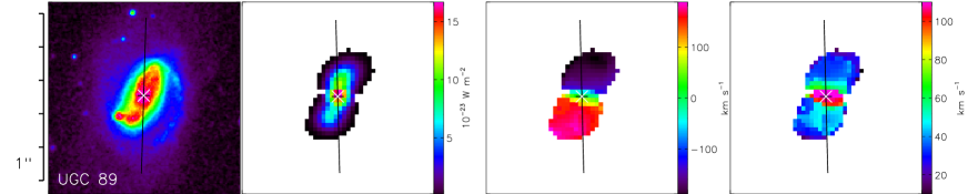
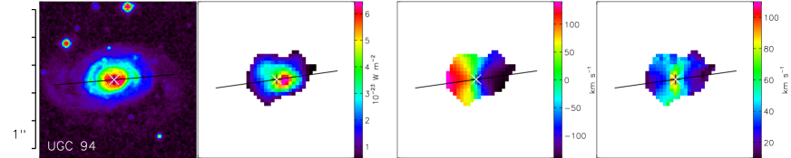
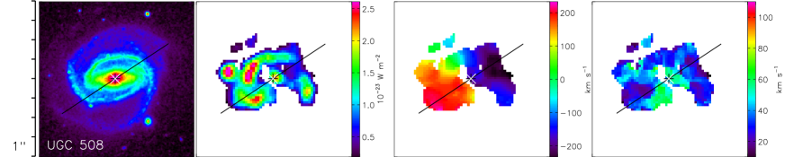
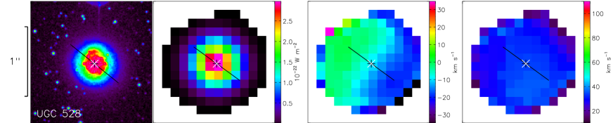
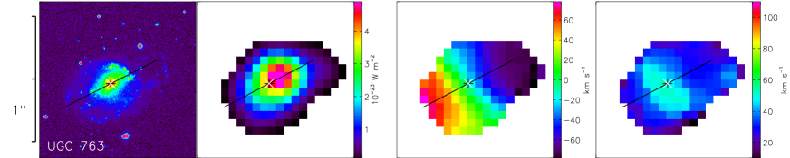
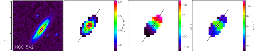
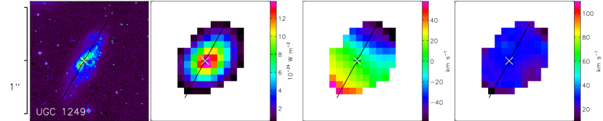
Figure 19: From left to rigth: XDSS image, H$\alpha$ monochromatic image, velocity field, velocity dispersion map. The white & black crosses mark the kinematical center. The black line is the major axis, its length represents the $D_{25}$. These maps are not truncated.

Appendix D Rotation curves

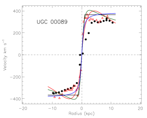
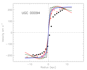
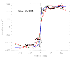
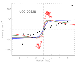
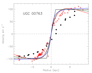
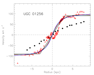
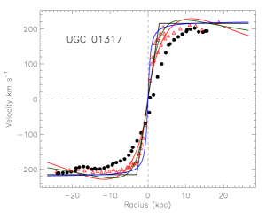
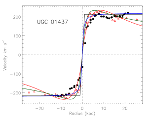
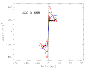
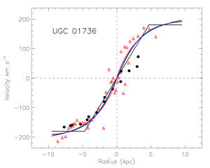
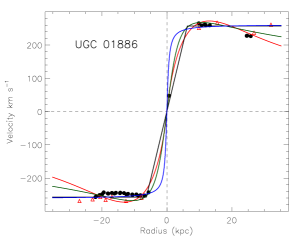
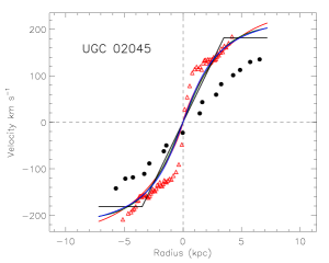
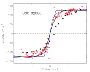
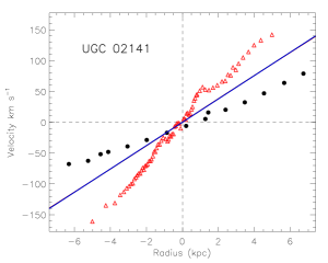
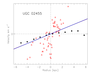
Figure 20: High redshift rotation curves along the major axis (black dots), actual rotation curves at redshift zero (red-open triangles) and high resolution rotation curve models (red line: exponential disk; green line: isothermal sphere; black line: “flat model”; blue line: arc-tangent function).

References

- Abraham et al. (1996) Abraham R. G., van den Bergh S., Glazebrook K., Ellis R. S., Santiago B. X., Surma P., Griffiths R. E., 1996, ApJS, 107, 1
- Amram et al. (2008) Amram P., Balkowski C., de Oliveira C. M., Plana H., Epinat B., 2008, in Wada K., Combes F., eds, Mapping the Galaxy and Nearby Galaxies From Nearby to High Redshift Compact Group of Galaxies. p. 261
- Amram et al. (2007) Amram P., Mendes de Oliveira C., Plana H., Balkowski C., Hernandez O., 2007, A&A, 471, 753
- Amram et al. (2004) Amram P., Mendes de Oliveira C., Plana H., Balkowski C., Hernandez O., Carignan C., Cypriano E. S., Sodré Jr. L., Gach J. L., Boulesteix J., 2004, ApJ, 612, L5
- Begeman (1987) Begeman K. G., 1987, PhD thesis, , Kapteyn Institute, (1987)
- Bertin & Arnouts (1996) Bertin E., Arnouts S., 1996, A&AS, 117, 393
- Blais-Ouellette et al. (1999) Blais-Ouellette S., Carignan C., Amram P., Côté S., 1999, AJ, 118, 2123
- Bosma (1978) Bosma A., 1978, PhD thesis, Groningen Universiteit
- Bournaud & Combes (2002) Bournaud F., Combes F., 2002, A&A, 392, 83
- Bournaud et al. (2008) Bournaud F., Daddi E., Elmegreen B. G., Elmegreen D. M., Nesvadba N., Vanzella E., di Matteo P., Le Tiran L., Lehnert M., Elbaz D., 2008, A&A, 486, 741
- Bournaud & Elmegreen (2009) Bournaud F., Elmegreen B. G., 2009, ApJ, 694, L158
- Bournaud et al. (2007) Bournaud F., Elmegreen B. G., Elmegreen D. M., 2007, ApJ, 670, 237
- Burbidge & Burbidge (1975) Burbidge E. M., Burbidge G. R., 1975, The Masses of Galaxies. Galaxies and the Universe, p. 81
- Catinella et al. (2006) Catinella B., Giovanelli R., Haynes M. P., 2006, ApJ, 640, 751
- Chapman et al. (1992) Chapman S., Pongracic H., Disney M., Nelson A., Turner J., Whitworth A., 1992, Nature, 359, 207
- Chemin et al. (2006) Chemin L., Balkowski C., Cayatte V., Carignan C., Amram P., Garrido O., Hernandez O., Marcelin M., Adami C., Boselli A., Boulesteix J., 2006, MNRAS, 366, 812
- Conselice et al. (2005) Conselice C. J., Blackburne J. A., Papovich C., 2005, ApJ, 620, 564
- Contini et al. (2009) Contini T. et al., 2009, in preparation
- Cresci et al. (2009) Cresci G., Hicks E. K. S., Genzel R. et al., 2009, ApJ, 697, 115
- Daddi et al. (2008) Daddi E., Dannerbauer H., Elbaz D., Dickinson M., Morrison G., Stern D., Ravindranath S., 2008, ApJ, 673, L21
- Daigle et al. (2006) Daigle O., Carignan C., Hernandez O., Chemin L., Amram P., 2006, MNRAS, 368, 1016
- de Vaucouleurs et al. (1992) de Vaucouleurs G., de Vaucouleurs A., Corwin Jr. H. G., Buta R. J., Paturel G., Fouque P., 1992, VizieR Online Data Catalog, 7137, 0
- Dekel et al. (2009) Dekel A., Birnboim Y., Engel G., Freundlich J., Goerdt T., Mumcuoglu M., Neistein E., Pichon C., Teyssier R., Zinger E., 2009, Nature, 457, 451
- Dickinson et al. (2003) Dickinson M., Papovich C., Ferguson H. C., Budavári T., 2003, ApJ, 587, 25
- Elmegreen et al. (2008) Elmegreen B. G., Bournaud F., Elmegreen D. M., 2008, ApJ, 688, 67
- Elmegreen & Elmegreen (2005) Elmegreen B. G., Elmegreen D. M., 2005, ApJ, 627, 632
- Elmegreen et al. (2007) Elmegreen D. M., Elmegreen B. G., Ravindranath S., Coe D. A., 2007, ApJ, 658, 763
- Epinat (2008a) Epinat B., 2008a, PhD thesis, Université de Provence (France)
- Epinat et al. (2008b) Epinat B., Amram P., Marcelin M., 2008b, MNRAS, 390, 466
- Epinat et al. (2008c) Epinat B., Amram P., Marcelin M., Balkowski C., Daigle O., Hernandez O., Chemin L., Carignan C., Gach J.-L., Balard P., 2008c, MNRAS, 388, 500
- Epinat et al. (2009a) Epinat B., Amram P., Marcelin M. et al., 2009a, in preparation
- Epinat et al. (2009b) Epinat B., Contini T., Le Fevre O., Vergani D., Amram P., Garilli B., Queyrel J., Tasca L., Tresse L., 2009b, accepted for publication in A&A, ArXiv e-prints 0903.1216
- Erb et al. (2003) Erb D. K., Shapley A. E., Steidel C. C., Pettini M., Adelberger K. L., Hunt M. P., Moorwood A. F. M., Cuby J.-G., 2003, ApJ, 591, 101
- Erb et al. (2004) Erb D. K., Steidel C. C., Shapley A. E., Pettini M., Adelberger K. L., 2004, ApJ, 612, 122
- Erb et al. (2006) Erb D. K., Steidel C. C., Shapley A. E., Pettini M., Reddy N. A., Adelberger K. L., 2006, ApJ, 647, 128
- Flores et al. (2006) Flores H., Hammer F., Puech M., Amram P., Balkowski C., 2006, A&A, 455, 107