Yield criteria for quasibrittle and frictional materials:
a generalization to surfaces with corners

Abstract

Convexity of a yield function (or phase-transformation function) and its relations to convexity of the corresponding yield surface (or phase-transformation surface) is essential to the invention, definition and comparison with experiments of new yield (or phase-transformation) criteria. This issue was previously addressed only under the hypothesis of smoothness of the surface, but yield surfaces with corners (for instance, the Hill, Tresca or Coulomb-Mohr yield criteria) are known to be of fundamental importance in plasticity theory. The generalization of a proposition relating convexity of the function and the corresponding surface to nonsmooth yield and phase-transformation surfaces is provided in this paper, together with the (necessary to the proof) extension of a theorem on nonsmooth elastic potential functions. While the former of these generalizations is crucial for yield and phase-transformation condition, the latter may find applications for potential energy functions describing phase-transforming materials, or materials with discontinuous locking in tension, or contact of a body with a discrete elastic/frictional support.

Keywords: yield surfaces; phase-transforming materials; phase-transforming surfaces; nonsmoothness of elastic energy; nonlinear elastic contact.

1 Introduction

$\bullet$ Yield or phase-transformation functions

Bigoni and Piccolroaz (2004) have proposed a new yield (or phase-transformation) function within the class of isotropic functions of the stress tensor $\sigma$ defined by

$$F(\mbox{\boldmath$\sigma$})=f(p)+\frac{q}{g(\theta)},$$ (1)

in which, having defined

$$\Phi=\frac{p+c}{p_{c}+c},$$ (2)

the meridian and deviatoric functions take the form

$$f(p)=\left\{\begin{array}[]{ll}-Mp_{c}\sqrt{\left(\Phi-\Phi^{m}\right)\left[2(1-\alpha)\Phi+\alpha\right]},&\Phi\in[0,1],\\[8.53581pt] +\infty,&\Phi\notin[0,1],\end{array}\right.\quad\frac{1}{g(\theta)}=\cos\left[\beta\frac{\pi}{6}-\frac{\cos^{-1}\left(\gamma\cos 3\theta\right)}{3}\right],$$ (3)

respectively, where $p,q$ and $\theta$ are stress invariants.

To preserve convexity of the yield surface, the seven material parameters defining the meridian shape function $f(p)$ and the deviatoric shape function $g(\theta)$ are restricted to range within the following intervals

$$M>0,\quad p_{c}>0,\quad c\geq 0,\quad 0<\alpha<2,\quad m>1,\quad 0\leq\beta\leq 2,\quad 0\leq\gamma\leq 1.$$ (6)

The interest in the above yield function and in the more general class of functions (1) lies in the fact that they can model the behaviour of many materials of engineering importance, such as ceramic (Piccolroaz et al. 2006) and metal (Bier and Hartmann, 2006; Hartmann and Bier, 2008; Heisserer et al. 2008) powders, metals (Hu and Wang (2005); Wierzbicki et al. 2005; Coppola and Folgarait, 2007), high strength alloys (for instance, Inconnel 718) (Bai and Wierzbicki, 2008), shape memory alloys (for instance, NiTi, NiAl, CuZnGa, or CuAlNi) (Raniecki and Mróz, 2008), concrete (Babua et al. 2005), and geomaterials (Dal Maso et al. 2007; Descamps and Tshibangu, 2007; DorMohammadi and Khoei 2008; Maiolino, 2005; Mortara, 2008; Sheldon et al. 2008). Moreover, eqn. (1) can be used as a general expression to set the condition for phase-transformations, for instance, to determine the stress threshold for martensitic or austenitic transformation (Raniecki and Lexcellent, 1998 and Lexcellent et al. 2002).

$\bullet$ Convexity of yield or phase-transformation functions

With reference to the class of functions (1), Bigoni and Piccolroaz (2004) have proved a general proposition providing necessary and sufficient conditions relating convexity of the yield function to convexity of the corresponding yield surface in the Haigh-Westergaard stress space (or principal stresses representation), a crucial property in the development of new expressions for yield or phase-transformation criteria. This proof is based on both the hypotheses of smoothness of the function $g(\theta)$, and validity of the smoothness limiting conditions $g^{\prime}(0)=0$ and $g^{\prime}(\pi/3)=0$, while as noticed by Laydi and Lexcellent (2009, see Appendix A.2 for a detailed discussion), the class of functions (1) –even under the particularizations (3)– may describe deviatoric yield surfaces with corners (Fig. 1), in which case the conditions for convexity provided by Bigoni and Piccolroaz (2004) remain only necessary but not sufficient. Since the convexity proposition is fundamental in developing new yield or phase-transformation criteria, it has immediately attracted a strong attention (Taillard et al. 2007; Laydi and Lexcellent, 2009; Lavernhe-Taillard et al. 2009; Saint-Sulpice et al. 2009; Valoroso and Rosati, 2009) and may definitely be important in analysing yield criteria with corners. Therefore, it becomes imperative to generalize the convexity proposition to nonsmooth deviatoric yield surfaces, which is obtained in the present article (Theorem 4.3, Section 4).

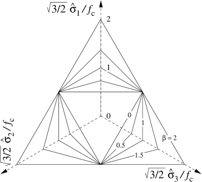
(a) (b)

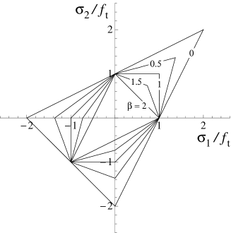
Figure 1: Examples of yield surfaces with corners obtained within the general class of yield function (1), namely $F(\mbox{\boldmath$\sigma$})=-f_{c}/g(\pi/3)+q/g(\theta)$ with the Bigoni and Piccolroaz (2004) deviatoric function, eqn. (3)₂, taking $\gamma=1$. (a) Deviatoric section: $\beta=0,0.5,1,1.5,2$. (b) Yield surface in the biaxial plane $\sigma_{1}/f_{t}$ vs. $\sigma_{2}/f_{t}$, with $\sigma_{3}=0$: $\beta=0,0.5,1,1.5,2$; $f_{t}$ and $f_{c}$ denote tensile and compressive uniaxial yield stress, respectively.

The generalization of the Bigoni and Piccolroaz (2004) proposition requires the generalization to nonregular functions of a theorem given by Hill (1968) regarding convexity of elastic strain potentials. In particular, Hill (1968) has shown that convexity of a smooth scalar isotropic function of a second-order symmetric tensor (a work-conjugate strain measure in his case) is equivalent to the convexity of the corresponding function of the principal values (the principal stretches in his case). The Hill’s theorem is of fundamental importance, since in many cases [for instance for the Ogden (1982) constitutive equations for rubber elasticity and the so-called ‘J₂–deformation theory materials’, Neale (1981)] constitutive equations of finitely-strained elastic materials are formulated with reference to the principal stretches and not with reference to the tensorial quantities, so that this theorem is usually reported in books (see for instance Ogden, 1984). Bigoni and Piccolroaz (2004) have recognized that the Hill’s theorem can be useful also for yield functions in plasticity theory, indeed the theorem has been duplicated (with a slightly different proof, without mentioning Hill’s theorem) in the context of elastoplasticity by Yang (1980). However, until now no generalization of the Hill’s theorem to nonregular functions has ever been given. Such a generalization may be relevant for elastic strain energy functions describing phase-transformation materials, or for elastic potential functions describing contact with discrete elastic asperities, or materials with discontinuous locking in tension (Fig. 2), but it is certainly of great interest for yield functions, which are often nonsmooth [for instance Hill (1950), Tresca and Coulomb-Mohr]. The generalization is provided in Section 3 and is the basis for the subsequent generalization of the Bigoni and Piccolroaz (2004) proposition to yield criteria (or transforming functions) with corners (Section 4).

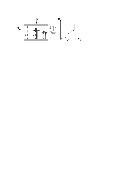
Figure 2: Contact with a nonlinear constraint. For $u<u^{*}$ the behaviour is linear elastic, while at $u=u^{*}$ and $u=u^{\circ}$ stiffness becomes infinite due to contact with frictional asperities obeying a rigid-plastic Coulomb rule. Although the sketched model is intrinsically inelastic, a representation restricted to the loading branch could be described by a continuous, convex and nonsmooth potential, for which Theorem 3.1 applies. In tension, a behaviour similar to that sketched on the right would correspond to a discontinuous locking mechanism of a material.

2 On smoothness of yield (or phase-transformation) functions

The conditions for smoothness of function $F(\mbox{\boldmath$\sigma$})$, eqn. (1), can be obtained by analysing the gradient of $F(\mbox{\boldmath$\sigma$})$,

$$\frac{\partial F}{\partial\mbox{\boldmath$\sigma$}}=-\frac{1}{3}f^{\prime}(p)\mbox{\boldmath$I$}+\sqrt{\frac{3}{2}}\frac{1}{g}\tilde{\mbox{\boldmath$S$}}-\sqrt{\frac{3}{2}}\frac{g^{\prime}}{g^{2}}\tilde{\mbox{\boldmath$S$}}^{\perp},$$ (7)

where $I$ is the identity tensor and

$$\tilde{\mbox{\boldmath$S$}}=\sqrt{\frac{3}{2}}\frac{\mbox{\boldmath$S$}}{q},\quad\tilde{\mbox{\boldmath$S$}}^{\perp}=\sqrt{\frac{2}{3}}q\frac{\partial\theta}{\partial\mbox{\boldmath$\sigma$}}=-\frac{3\sqrt{3}}{\sqrt{2}q^{2}\sin 3\theta}\left[\mbox{\boldmath$S$}^{2}-\frac{2}{9}q^{2}\mbox{\boldmath$I$}-\frac{q}{3}\cos 3\theta\mbox{\boldmath$S$}\right].$$ (8)

Note that:

• $\tilde{\mbox{\boldmath$S$}}$ is discontinuous along the hydrostatic axis, but this discontinuity does not affect convexity of $F(\mbox{\boldmath$\sigma$})$, see Lemma 4.1;

• $\tilde{\mbox{\boldmath$S$}}^{\perp}$ is discontinuous along the hyperplanes defined by $\theta=0$ and $\theta=\pi/3$. This discontinuity can be eliminated for functions $g$ such that $g^{\prime}=0$ at $\theta=0$ and $\theta=\pi/3$, which is the case of many yield functions, for instance, all yield functions described by eqn. (3)₂ when $0\leq\gamma<1$. The analysis of the nonsmooth case, at $\theta=0$ and $\theta=\pi/3$ is the main target of the present article and leads to Theorem 4.1, which is generalized into Theorem 4.2 and finally leads to Theorem 4.3.

We analyse now smoothness of the deviatoric part $q/g(\theta)$ as a function of $S_{1},S_{2}$, where $S_{1},S_{2}$ denote two principal values of the deviatoric stress. Assuming that $g(\theta)$ is continuous and strictly positive in $[0,\pi/3]$, and smooth everywhere in $(0,\pi/3)$, the gradient of $q/g(\theta)$ with respect to the variables $S_{1},S_{2}$ is given by

$$\frac{\partial q/g(\theta)}{\partial S_{i}}=\frac{1}{g(\theta)}\frac{\partial q}{\partial S_{i}}-q\frac{g^{\prime}(\theta)}{g^{2}(\theta)}\frac{\partial\theta}{\partial S_{i}},\qquad i=1,2,$$ (9)

where

$$\frac{\partial q}{\partial S_{i}}=\frac{3}{2q}[2S_{i}-(-1)^{i}m_{i}],\qquad i=1,2,$$ (10)

$$\frac{\partial\theta}{\partial S_{i}}=-\frac{3\sqrt{3}}{2q^{2}}\hat{H}(S_{1},S_{2})m_{i},\qquad i=1,2,$$ (11)

in which the indices are not summed and the vector $m$ has the components: $\{\mbox{\boldmath$m$}\}=\{S_{2},-S_{1}\}$.

The function $\hat{H}(S_{1},S_{2})$ is a piecewise constant function defined by

$$\hat{H}(S_{1},S_{2})=\frac{(S_{1}-S_{2})(2S_{1}+S_{2})(S_{1}+2S_{2})}{\sqrt{(S_{1}-S_{2})^{2}(2S_{1}+S_{2})^{2}(S_{1}+2S_{2})^{2}}}=\mathop{\mathrm{sign}}[(S_{1}-S_{2})(2S_{1}+S_{2})(S_{1}+2S_{2})],$$ (12)

which takes the values $1$ or $-1$ only, Fig. 3.

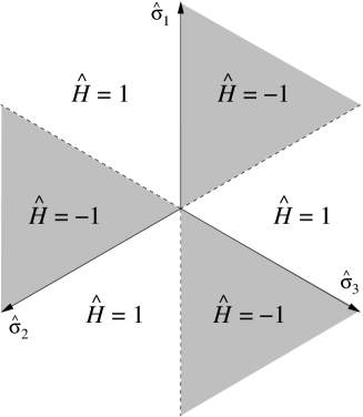
Figure 3: Plot of the function $\hat{H}$, eqn. (12), in the deviatoric plane. Axes $\hat{\sigma}_{1},\hat{\sigma}_{2},\hat{\sigma}_{3}$ are the projections of the principal stress axes onto the deviatoric plane.

We may note from Fig. 3 that the function $\hat{H}(S_{1},S_{2})$ is discontinuous along the projections of the principal stress axes on the deviatoric plane:

$$\text{axis }\hat{\sigma}_{1}:\{S_{1},-S_{1}/2,-S_{1}/2\},\quad\text{if }S_{1}>0\text{ then }\theta=0,\quad\text{if }S_{1}<0\text{ then }\theta=\pi/3,$$

$$\text{axis }\hat{\sigma}_{2}:\{-S_{2}/2,S_{2},-S_{2}/2\},\quad\text{if }S_{2}>0\text{ then }\theta=0,\quad\text{if }S_{2}<0\text{ then }\theta=\pi/3,$$ (13)

$$\text{axis }\hat{\sigma}_{3}:\{-S_{3}/2,-S_{3}/2,S_{3}\},\quad\text{if }S_{3}>0\text{ then }\theta=0,\quad\text{if }S_{3}<0\text{ then }\theta=\pi/3.$$

Accordingly,

the function $q/g(\theta)$ is smooth if and only if $g(\theta)$ is smooth everywhere in $(0,\pi/3)$ and $g^{\prime}(0)=g^{\prime}(\pi/3)=0$, see Fig. 4.

(a)       (b)

Figure 4: Conditions for smoothness of the yield surface deviatoric section. (a) At $\theta=0$: $g^{\prime}(0)=0$. (b) At $\theta=\pi/3$: $g^{\prime}(\pi/3)=0$.

3 Nonsmooth, convex and isotropic functions

With reference to elastic potential of finite-strain constitutive equations, Hill (1968) has proven that convexity of a smooth scalar isotropic function of a second-order symmetric tensor (a work-conjugate strain measure in his case) is equivalent to the convexity of the corresponding function of the principal values (the principal stretches in his case). The Hill’s theorem is of fundamental importance, since in many cases constitutive equations of finitely-strained elastic materials are formulated with reference to the principal stretches and not with reference to the tensorial quantities, see for instance Ogden (1984). Bigoni and Piccolroaz (2004) have evidenced that the Hill’s theorem also applies to yield functions in elastoplasticity theory.

Until now, no generalization of the Hill’s theorem to nonsmooth function has ever been given. As mentioned in the Introduction, such a generalization may be relevant for elastic strain energy functions describing phase-transformation materials (although in those cases usually non-convexity is employed), or for potential functions describing discontinuous locking in tension, or contact with discrete elastic springs (as explained in Fig. 2, where contact of a rigid punch with a linear elastic set of springs having different heights and rigid/frictional devices is envisaged. The loading branch of this model can be described through a piecewise linear and convex strain energy function).

In any case, the generalization of the Hill’s theorem is certainly of great interest for yield functions, which are often nonsmooth, as for instance in the cases of the Hill (1950), Tresca, modified-Tresca, and Coulomb-Mohr yield surfaces. The generalization is provided in this Section.

We begin with a simple lemma.

Lemma 3.1.

Let us consider a scalar isotropic function $\phi$ of tensorial argument $\sigma_{ij}\in\mathsf{Sym}$ and the corresponding function $\tilde{\phi}$ written with reference to the principal values $\sigma_{i}$:

$$\phi(\sigma_{11},\sigma_{22},\sigma_{33},\sigma_{12},\sigma_{13},\sigma_{23})=\tilde{\phi}(\sigma_{1},\sigma_{2},\sigma_{3}),$$

then, due to isotropy, the following equality holds

$$\tilde{\phi}(\sigma_{1},\sigma_{2},\sigma_{3})=\phi(\sigma_{1},\sigma_{2},\sigma_{3},0,0,0),$$ (14)

so that $\tilde{\phi}$ is the restriction of $\phi$ to the subdomain of diagonal tensors.

Proof.

The property (14) is easily proven by the following consideration. The isotropy of $\phi(\mbox{\boldmath$\sigma$})$ implies that the function $\phi(\mbox{\boldmath$\sigma$})$ is equal to a function $\hat{\phi}$ of the invariants of $\sigma$,

$$\phi(\sigma_{11},\sigma_{22},\sigma_{33},\sigma_{12},\sigma_{13},\sigma_{23})=\hat{\phi}(\mathop{\mathrm{tr}}\mbox{\boldmath$\sigma$},\mathop{\mathrm{tr}}\mbox{\boldmath$\sigma$}^{2},\mathop{\mathrm{tr}}\mbox{\boldmath$\sigma$}^{3}),$$

and thus

$$\tilde{\phi}(\sigma_{1},\sigma_{2},\sigma_{3})=\hat{\phi}(\mathop{\mathrm{tr}}\mbox{\boldmath$\sigma$},\mathop{\mathrm{tr}}\mbox{\boldmath$\sigma$}^{2},\mathop{\mathrm{tr}}\mbox{\boldmath$\sigma$}^{3})=\phi(\sigma_{1},\sigma_{2},\sigma_{3},0,0,0).$$

∎

We need now to introduce the notion of subdifferential (or subgradient), which will be used in the sequel for the generalization of the Hill (1968) theorem to nonsmooth functions.

A function $\phi:\,U\subseteq\mathbb{R}^{n}\rightarrow\mathbb{R}$ is convex if and only if the subdifferential

$$\partial\phi(\mbox{\boldmath$X$}_{0})=\left\{\mbox{\boldmath$Q$}\in\mathbb{R}^{n}:\,\phi(\mbox{\boldmath$X$})-\phi(\mbox{\boldmath$X$}_{0})\geq\mbox{\boldmath$Q$}\mbox{\boldmath$\,\cdot\,$}(\mbox{\boldmath$X$}-\mbox{\boldmath$X$}_{0}),\quad\forall\mbox{\boldmath$X$}\in U\right\},$$ (15)

is defined and non empty at every point $\mbox{\boldmath$X$}_{0}$ of its domain $U$.

Note that although the subgradient is a set of vectors, in the sequel we shall denote with the term ‘subgradient’ both the set itself and its elements.

The following lemma, necessary to the proof of Theorem (3.1), is similar to the analogous given by Hill (1968), but now it has been generalized and extended to nonsmooth isotropic functions.

Lemma 3.2.

Given a convex function of the principal stresses, $\tilde{\phi}(\sigma_{1},\sigma_{2},\sigma_{3})$, the algebraic order of components of the subgradient $(Q_{1},Q_{2},Q_{3})$ at $(\sigma_{1},\sigma_{2},\sigma_{3})$ is the same as $(\sigma_{1},\sigma_{2},\sigma_{3})$.

Proof.

From the strict convexity of $\tilde{\phi}$, it follows that

$$\sum_{i=1}^{3}(Q_{i}-Q_{i}^{0})(\sigma_{i}-\sigma_{i}^{0})>0,$$ (16)

$\forall(Q_{1},Q_{2},Q_{3})\in\partial\tilde{\phi}(\sigma_{1},\sigma_{2},\sigma_{3})$ and $\forall(Q_{1}^{0},Q_{2}^{0},Q_{3}^{0})\in\partial\tilde{\phi}(\sigma_{1}^{0},\sigma_{2}^{0},\sigma_{3}^{0})$. Choosing $(\sigma_{2}^{0},\sigma_{1}^{0},\sigma_{3}^{0})=(\sigma_{1},\sigma_{2},\sigma_{3})$ and taking into account isotropy, it follows that

$$(Q_{1}-Q_{2})(\sigma_{1}-\sigma_{2})>0,$$ (17)

and similarly for each of the other pairs. It follows that the vector $(Q_{1},Q_{2},Q_{3})$ is ordered in the same algebraic order as $(\sigma_{1},\sigma_{2},\sigma_{3})$, a property which remains true also assuming convexity ‘$\geq$’ instead of strict convexity ‘$>$’. ∎

Note also that we will make use in the proof of Theorem 3.1 of an auxiliary property of the scalar product between two symmetric tensors, first noticed by Hill (1968):

“if their eigenvalues are given, but their axes are directly arbitrarily, the product attains its greatest value when the major and minor axes are pairwise coincident.”

We refer to Appendix A.1 for a detailed discussion and proof of this auxiliary property.

Theorem 3.1.

Extension of the Hill (1968) theorem to nonregular functions. Convexity of an isotropic (not necessarily smooth) function of a symmetric (stress) tensor $\sigma$ is equivalent to convexity of the corresponding function of the principal (stress) values $\sigma_{i}$ ($i=1,2,3$). In symbols, given:

$$\phi(\mbox{\boldmath$\sigma$})=\tilde{\phi}(\sigma_{1},\sigma_{2},\sigma_{3}),$$ (18)

then $\forall\mbox{\boldmath$\sigma$}\in\mathsf{Sym}$,

$$\exists\mbox{\boldmath$Q$}\in\mathsf{Sym}:\ \phi(\mbox{\boldmath$\sigma$}^{\prime})-\phi(\mbox{\boldmath$\sigma$})\geq\mbox{\boldmath$Q$}\cdot\left(\mbox{\boldmath$\sigma$}^{\prime}-\mbox{\boldmath$\sigma$}\right),\quad\forall\mbox{\boldmath$\sigma$}^{\prime}\in\mathsf{Sym},$$ (19)

$$\Updownarrow$$

$$\exists(Q_{1},Q_{2},Q_{3})\in\mathbb{R}^{3}:\ \tilde{\phi}(\sigma_{1}^{\prime},\sigma_{2}^{\prime},\sigma_{3}^{\prime})-\tilde{\phi}(\sigma_{1},\sigma_{2},\sigma_{3})\geq\sum_{i=1}^{3}Q_{i}\left(\sigma_{i}^{\prime}-\sigma_{i}\right),\quad\forall(\sigma_{1}^{\prime},\sigma_{2}^{\prime},\sigma_{3}^{\prime})\in\mathbb{R}^{3}.$$ (20)

Proof.

The proof that (19) $\Longrightarrow$ (20) follows immediately from the property (14). The converse (20) $\Longrightarrow$ (19) is not trivial and is proven in the following.

We denote by $(\sigma_{1},\sigma_{2},\sigma_{3})$ the principal values of a given $\sigma$ and by $(Q_{1},Q_{2},Q_{3})$ the subgradient of $\tilde{\phi}$ at $(\sigma_{1},\sigma_{2},\sigma_{3})$. We define now $\mbox{\boldmath$Q$}\in\mathsf{Sym}$ to be

$$\mbox{\boldmath$Q$}=Q_{1}\mbox{\boldmath$q$}_{1}\otimes\mbox{\boldmath$q$}_{1}+Q_{2}\mbox{\boldmath$q$}_{2}\otimes\mbox{\boldmath$q$}_{2}+Q_{3}\mbox{\boldmath$q$}_{3}\otimes\mbox{\boldmath$q$}_{3},$$

where $\{\mbox{\boldmath$q$}_{1},\mbox{\boldmath$q$}_{2},\mbox{\boldmath$q$}_{3}\}$ is an orthonormal basis of $\mathbb{R}^{3}$. Then, assuming that $(\sigma_{1}^{\prime},\sigma_{2}^{\prime},\sigma_{3}^{\prime})$ are numbered in the same algebraic order as $(\sigma_{1},\sigma_{2},\sigma_{3})$, and since from the Lemma 3.2 we know that the algebraic order of $(Q_{1},Q_{2},Q_{3})$ is also the same as $(\sigma_{1},\sigma_{2},\sigma_{3})$, the auxiliary property of the scalar product (proven in Appendix A.1), implies that

$$\sum_{i=1}^{3}Q_{i}\left(\sigma_{i}^{\prime}-\sigma_{i}\right)\geq\mbox{\boldmath$Q$}\cdot(\mbox{\boldmath$\sigma$}^{\prime}-\mbox{\boldmath$\sigma$}),\quad\forall\mbox{\boldmath$\sigma$}^{\prime}\in\mathsf{Sym}.$$ (21)

Since, by hypothesis, the following equation holds true

$$\phi(\mbox{\boldmath$\sigma$}^{\prime})-\phi(\mbox{\boldmath$\sigma$})=\tilde{\phi}(\sigma_{1}^{\prime},\sigma_{2}^{\prime},\sigma_{3}^{\prime})-\tilde{\phi}(\sigma_{1},\sigma_{2},\sigma_{3})\geq\sum_{i=1}^{3}Q_{i}\left(\sigma_{i}^{\prime}-\sigma_{i}\right),\quad\forall(\sigma_{1}^{\prime},\sigma_{2}^{\prime},\sigma_{3}^{\prime})\in\mathbb{R}^{3},$$ (22)

eqn. (21) guarantees that $\mbox{\boldmath$Q$}\in\partial\phi(\mbox{\boldmath$\sigma$})$, so that $\phi(\mbox{\boldmath$\sigma$})$ results to be convex. ∎

4 Convexity of yield functions with corners

We begin with proving that the discontinuity of the yield function gradient along the hydrostatic axis [see eqn. (8)] is inconsequential on convexity.

Lemma 4.1.

The convexity of the function $q/g(\theta)$ is unaffected by the fact that $\tilde{\mbox{\boldmath$S$}}$ and $\tilde{\mbox{\boldmath$S$}}^{\perp}$ defined in eqn. (8) are discontinuous along the hydrostatic axis, where $S_{1}=S_{2}=0$.

Proof.

From the definition of convexity, it follows that (van Tiel, 1984)

$\displaystyle q/g(\theta)$ is convex at $(S_{1},S_{2})$ $\Leftrightarrow$ for every line $t$ through $(S_{1},S_{2})$, the restriction to $t$ of $\displaystyle q/g(\theta)$ is convex

Let us consider all deviatoric lines through the point $\{S_{1}=0,S_{2}=0\}$, these can be represented (using parameter $\epsilon$ and slope $k$) as $\{\epsilon,k\,\epsilon\}$. The restriction of $q/g(\theta)$ to these lines is a function $h(\epsilon)$, whose derivative with respect to $\epsilon$ is

$$h^{\prime}(\epsilon)=\left\{\frac{\nabla q}{g}-q\frac{g^{\prime}}{g^{2}}\nabla\theta\right\}\mbox{\boldmath$\,\cdot\,$}\{1,k\},$$ (23)

where $\nabla$ denotes the gradient taken with respect to the variables $\{S_{1},S_{2}\}$, so that, since $\nabla\theta\mbox{\boldmath$\,\cdot\,$}\{1,k\}=0$ and

$$q=|\epsilon|\sqrt{3}\sqrt{1+k+k^{2}},\quad\nabla q=\frac{\sqrt{3}\,\mathop{\mathrm{sign}}{\epsilon}}{\sqrt{1+k+k^{2}}}\{2+k,1+2k\},$$ (24)

we obtain

$$h^{\prime}(\epsilon)=\frac{\sqrt{3}\,\mathop{\mathrm{sign}}{\epsilon}}{g}\sqrt{1+k+k^{2}}.$$ (25)

At a singular point, convexity requires that

$$\lim_{\epsilon\rightarrow 0^{-}}h^{\prime}(\epsilon)<\lim_{\epsilon\rightarrow 0^{+}}h^{\prime}(\epsilon),$$ (26)

which is always satisfied, so that the discontinuities in $\tilde{\mbox{\boldmath$S$}}$ and $\tilde{\mbox{\boldmath$S$}}^{\perp}$ along the hydrostatic axis are inconsequential on convexity. ∎

With reference to the deviatoric part $q/g(\theta)$ of the yield function (1), we give now necessary and sufficient conditions (Theorem 4.1) for equivalence between convexity of yield functions and convexity of yield surface. To this purpose, we first need the following lemma.

Lemma 4.2.

Given a generic isotropic function $\phi$ of the stress that can be expressed as

$$\tilde{\phi}(\sigma_{1},\sigma_{2},\sigma_{3})=\hat{\phi}(S_{1},S_{2}),$$ (27)

where $S_{1}$ and $S_{2}$ are two of the principal components of the deviatoric stress, i.e.

$$S_{1}=\frac{1}{3}\left(2\sigma_{1}-\sigma_{2}-\sigma_{3}\right),\quad S_{2}=\frac{1}{3}\left(-\sigma_{1}+2\sigma_{2}-\sigma_{3}\right),$$ (28)

convexity of $\tilde{\phi}(\sigma_{1},\sigma_{2},\sigma_{3})$ is equivalent to convexity of $\hat{\phi}(S_{1},S_{2})$.

Proof.

This proposition follows immediately from the fact that the relation (28) between $\{S_{1},S_{2}\}$ and $\{\sigma_{1},\sigma_{2},\sigma_{3}\}$ is linear. ∎

The following theorem is the generalization of Lemma 3 by Bigoni and Piccolroaz (2004) to the case of nonsmooth deviatoric sections of the yield surface. Note that the difference between the two versions of the theorem lies on the two conditions $g^{\prime}(0)\leq 0$ and $g^{\prime}(\pi/3)\geq 0$. A consequence of the following theorem is that the convexity conditions by Laydi and Lexcellent (2009) are only sufficient (but not necessary) for convexity of smooth functions (see Appendix A.2).

Theorem 4.1.

Convexity of nonsmooth deviatoric representation $q/g(\theta)$ vs. convexity of the deviatoric section of the yield surface.

Assuming that $g(\theta)$ is continuous and strictly positive in $[0,\pi/3]$ and twice-differentiable everywhere in $(0,\pi/3)$, convexity of

$$\frac{q}{g(\theta)}$$ (29)

as a function of $S_{1},S_{2}$ is equivalent to the convexity of the deviatoric section in the Haigh-Westergaard space:

$$g^{2}+2g^{\prime 2}-gg^{\prime\prime}\geq 0,\quad\forall\theta\in(0,\pi/3)\quad\text{and}\quad g^{\prime}(0)\leq 0,\quad g^{\prime}(\pi/3)\geq 0.$$ (30)

Proof.

Let us define $\Omega$ as the set of all points $\{S_{1},S_{2}\}$ not on the axes $\hat{\sigma}_{1},\hat{\sigma}_{2},\hat{\sigma}_{3}$, see eqns. (13). The theorem is proven first (point 1 below) by showing local convexity at all points of $\Omega$ (regular points) and, second (point 2 below), considering the points of $\partial\Omega$, i.e. the axes $\hat{\sigma}_{1},\hat{\sigma}_{2},\hat{\sigma}_{3}$, where the function has corners (singular points).

• Local convexity in $\Omega$ (for which $0<\theta<\pi/3$).

  The function $q/g(\theta)$ is $C^{2}(\Omega)$, so that we can apply the convexity criterion based on the Hessian.

  The Hessian of the function (29) is

  $$\frac{\partial^{2}q/g(\theta)}{\partial S_{i}\partial S_{j}}=\frac{1}{g^{3}}\left[g^{2}\frac{\partial^{2}q}{\partial S_{i}\partial S_{j}}+q(2g^{\prime}\,{}^{2}-gg^{\prime\prime})\frac{\partial\theta}{\partial S_{i}}\frac{\partial\theta}{\partial S_{j}}-gg^{\prime}\left(\frac{\partial q}{\partial S_{i}}\frac{\partial\theta}{\partial S_{j}}+\frac{\partial q}{\partial S_{j}}\frac{\partial\theta}{\partial S_{i}}+q\frac{\partial^{2}\theta}{\partial S_{i}\partial S_{j}}\right)\right],$$ (31)

  where $i$ and $j$ range between 1 and 2 and all functions $q$ and $\theta$ are to be understood as functions of $S_{1}$ and $S_{2}$ only. The Hessian of $q$ may be easily calculated to be

  $$\frac{\partial^{2}q}{\partial S_{i}\partial S_{j}}=\frac{27}{4q^{3}}m_{i}m_{j},$$

  where indices are not summed and $\{\mbox{\boldmath$m$}\}=\{S_{2},-S_{1}\}$. The Hessian of $\theta$ becomes

  $$\frac{\partial^{2}\theta}{\partial S_{i}\partial S_{j}}=\frac{-1}{3\sin 3\theta}\left(\frac{\cos 3\theta}{\sin^{2}3\theta}\frac{\partial\cos 3\theta}{\partial S_{i}}\frac{\partial\cos 3\theta}{\partial S_{j}}+\frac{\partial^{2}\cos 3\theta}{\partial S_{i}\partial S_{j}}\right),$$

  so that

  $$\frac{\partial q}{\partial S_{i}}\frac{\partial\theta}{\partial S_{j}}+\frac{\partial q}{\partial S_{j}}\frac{\partial\theta}{\partial S_{i}}+q\frac{\partial^{2}\theta}{\partial S_{i}\partial S_{j}}=\frac{-1}{3\sin 3\theta}\left[\frac{\partial^{2}q\cos 3\theta}{\partial S_{i}\partial S_{j}}-\cos 3\theta\frac{\partial^{2}q}{\partial S_{i}\partial S_{j}}+q\frac{\cos 3\theta}{\sin^{2}3\theta}\frac{\partial\cos 3\theta}{\partial S_{i}}\frac{\partial\cos 3\theta}{\partial S_{j}}\right],$$ (32)

  where

  $$\frac{\partial\cos 3\theta}{\partial S_{i}}=\frac{9\sqrt{3}\sin 3\theta}{2q^{2}}\hat{H}(S_{1},S_{2})m_{i},\quad\frac{\partial^{2}q\cos 3\theta}{\partial S_{i}\partial S_{j}}=-27^{2}\frac{J_{3}}{q^{6}}m_{i}m_{j}.$$ (33)

  A substitution of (33) into (32) yields

  $${\frac{\partial q}{\partial S_{i}}\frac{\partial\theta}{\partial S_{j}}+\frac{\partial q}{\partial S_{j}}\frac{\partial\theta}{\partial S_{i}}+q\frac{\partial^{2}\theta}{\partial S_{i}\partial S_{j}}}=0,$$ (34)

  so that we may conclude that the Hessian (31) can be written as

  $$\frac{\partial^{2}q/g(\theta)}{\partial S_{i}\partial S_{j}}=\frac{27}{4}\frac{\left(g^{2}+2g^{\prime}\,{}^{2}-gg^{\prime\prime}\right)}{q^{3}g^{3}}m_{i}\,m_{j},$$ (35)

  from which condition $g^{2}+2g^{\prime}\,{}^{2}-gg^{\prime\prime}\geq 0$ is immediately obtained.

• Local convexity on $\partial\Omega$ (for which $\theta=0$ or $\theta=\pi/3$).

  We consider in the following only the axis $\hat{\sigma}_{1}$, since the proof remains strictly similar for the other axes.

  • Case $\theta=0$.

    A line $t$ through $(1,-1/2)$ has the parametric representation $\{(1+\epsilon,-1/2+k\epsilon)|\epsilon\in\mathbb{R}\}$, where $\epsilon$ is the parameter and $k$ is the slope of the line. Using this representation, the restriction to $t$ of $q/g(\theta)$ is a function $h(\epsilon)$, whose derivative is given by eqn. (23). From the limits

    $$q\to 3/2,\quad\nabla q\to\{-3/2,0\}\quad\text{and}\quad\nabla\theta\to\pm\frac{1+2k}{|1+2k|\sqrt{3}}\{1,2\}\quad\text{as}\quad\epsilon\to 0^{\pm},$$ (36)

    we derive

    $$h^{\prime}_{\pm}(0)=\frac{3}{2g}\mp\frac{\sqrt{3}}{2}|1+2k|\frac{g^{\prime}(0)}{g^{2}(0)}.$$ (37)

    so that the convexity condition for $h(\epsilon)$ at $\epsilon=0$, namely, $h^{\prime}_{-}(0)<h^{\prime}_{+}(0)$ is equivalent to $g^{\prime}(0)<0$.

  • Case $\theta=\pi/3$.

    A line $t$ through $(-1,1/2)$ has the representation $\{(-1+\epsilon,1/2+k\epsilon)|\epsilon\in\mathbb{R}\}$, where $k$ is the slope of the line. Using this representation, the restriction to $t$ of $q/g(\theta)$ is a function $h(\epsilon)$, whose derivative is given by eqn. (23). From the limits

    $$q\to 3/2,\quad\nabla q\to\{-3/2,0\}\quad\text{and}\quad\nabla\theta\to\mp\frac{1+2k}{|1+2k|\sqrt{3}}\{1,2\}\quad\text{as}\quad\epsilon\to 0^{\pm},$$ (38)

    we derive

    $$h^{\prime}_{\pm}(0)=-\frac{3}{2g}\pm\frac{\sqrt{3}}{2}|1+2k|\frac{g^{\prime}(0)}{g^{2}(0)},$$ (39)

    so that the convexity condition for $h(\epsilon)$ at $\epsilon=0$, $h^{\prime}_{-}(0)<h^{\prime}_{+}(0)$ is equivalent to $g^{\prime}(\pi/3)>0$.

Since $q/g(\theta)$ is locally convex in the sets $\Omega$ and $\partial\Omega$, the proof is concluded by noting that $\Omega\cup\partial\Omega$ represents the whole deviatoric plane, so that $q/g(\theta)$ is globally convex.

∎

There are yield surfaces, for instance that proposed by Hill (1950), see Fig. 5 (a), presenting corners for values of $\theta$ internal to the interval $(0,\pi/3)$. In particular, assuming a piecewise smooth function $g(\theta)$, the Hill (1950) criterion can be formulated within the general class of yield functions (1), namely, introducing the yield stress in uniaxial compression $-f_{c}$, by $F(\mbox{\boldmath$\sigma$})=-f_{c}+q/g(\theta)$, where

$$\frac{1}{g(\theta)}=\left\{\begin{array}[]{ll}\displaystyle\cos\left[-\frac{1}{3}\cos^{-1}(\cos 3\theta)\right],&\displaystyle 0\leq\theta\leq\pi/6,\\[14.22636pt] \displaystyle\cos\left[\frac{\pi}{3}-\frac{1}{3}\cos^{-1}(\cos 3\theta)\right],&\displaystyle\pi/6<\theta\leq\pi/3.\end{array}\right.$$ (40)

Another example of a deviatoric section with corners in $\theta=0$, $\theta=\pi/3$, and $\theta=\theta_{1}=7\pi/30$ is given by $F(\mbox{\boldmath$\sigma$})=-f_{c}/g(\pi/3)+q/g(\theta)$, with

$$g(\theta)=\left\{\begin{array}[]{ll}\displaystyle\frac{\cos\left[\pi/12-1/3\cos^{-1}(\cos 3\theta_{1})\right]}{\cos\left[\pi/12-1/3\cos^{-1}(\cos 3\theta)\right]},&\displaystyle 0\leq\theta\leq\theta_{1},\\[14.22636pt] \displaystyle\frac{\cos\left[\pi/4-1/3\cos^{-1}(\cos 3\theta_{1})\right]}{\cos\left[\pi/4-1/3\cos^{-1}(\cos 3\theta)\right]},&\displaystyle\theta_{1}<\theta\leq\pi/3,\end{array}\right.$$ (41)

which is plotted in Fig. 5 (b).

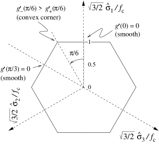
(a)       (b)

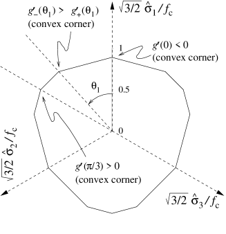
Figure 5: Yield surface deviatoric sections presenting corners for values of $\theta$ internal to the interval $(0,\pi/3)$: (a) Yield criterion proposed by Hill (1950), described by eqn. (40). (b) Yield criterion described by eqn. (41).

It is clear from the above examples that employing the function $g(\theta)$ defined by eqn. (3)₂, with different values of parameter $\beta$ on a finite number of subintervals of $\theta\in[0,\pi/3]$, it is possible to represent all possible nonsmooth deviatoric sections of a yield surface. This statement justifies the interest in the following theorem, covering the situations in which the yield surface presents corners for values of $\theta$ internal to $(0,\pi/3)$.

Theorem 4.2.

Convexity of piecewise-smooth deviatoric representation $g(\theta)$ vs. convexity of the deviatoric section of the yield surface.

Assuming that $g(\theta)$ is continuous and strictly positive in $[0,\pi/3]$ and twice-differentiable almost everywhere in $(0,\pi/3)$, and denoting by $\theta_{i}\in(0,\pi/3)$ the singular points of $g(\theta)$, convexity of

$$\frac{q}{g(\theta)}$$ (42)

as a function of $S_{1},S_{2}$ is equivalent to the convexity of the deviatoric section in the Haigh-Westergaard space:

$$g^{2}+2g^{\prime 2}-gg^{\prime\prime}\geq 0,\quad\forall\theta\in(0,\pi/3)-\{\theta_{i}\}\quad\text{and}\quad g^{\prime}(0)\leq 0,\quad g^{\prime}(\pi/3)\geq 0,$$ (43)

and

$$g^{\prime}_{-}(\theta_{i})>g^{\prime}_{+}(\theta_{i}),\quad\forall\theta_{i}.$$ (44)

Proof.

Conditions (43) have been already proven in Theorem 4.1 and do not need further explanation. We therefore restrict our attention to the singular points $\theta_{i}$, to derive condition (44).

We consider a generic point in the first $\pi/3$-sector of the deviatoric plane (taken clockwise from axis $\hat{\sigma}_{1}$; the proof can be easily extended to the other sectors), $2q/3\{\cos\theta,-\cos(\pi/3-\theta)\}$, and the parametric representation (with the parameter $\epsilon$) of all lines of slope $k$ through this point (Fig. 6)

$$\left\{\frac{2}{3}q\cos\theta+\epsilon,-\frac{2}{3}q\cos\left(\frac{\pi}{3}-\theta\right)+k\epsilon\right\}.$$ (45)

The derivative of the restriction $h$ of $q/g(\theta)$ to this line is again given by eqn. (23), with all the functions calculated at points (45). Taking the limit values at $\epsilon=0$,

$$\nabla q=\left\{\frac{3}{2}\cos\theta-\frac{\sqrt{3}}{2}\sin\theta,-\sqrt{3}\sin\theta\right\},\quad\nabla\theta=\frac{\sqrt{3}}{q}\hat{H}\left\{\cos\left(\frac{\pi}{3}-\theta\right),\cos\theta\right\},$$ (46)

and noting that $\hat{H}=-1$ in the $\pi/3$-sector under consideration (see Fig. 3), we obtain

$$\lim_{\epsilon\rightarrow 0^{\pm}}h^{\prime}(\epsilon)=\frac{\sqrt{3}}{2\,g(\theta)}\left[\sqrt{3}\cos\theta-(1+2k)\sin\theta\right]-\frac{\sqrt{3}}{2}\frac{g^{\prime}_{(*)}(\theta)}{g^{2}(\theta)}\hat{H}\left[(1+2k)\cos\theta+\sqrt{3}\sin\theta\right],$$ (47)

where

$$(*)=\left\{\begin{array}[]{lll}\pm&\mbox{for}&\displaystyle-\infty<k<-\frac{\cos\left(\pi/3-\theta\right)}{\cos\theta},\\[14.22636pt] \mp&\mbox{for}&\displaystyle-\frac{\cos\left(\pi/3-\theta\right)}{\cos\theta}<k<+\infty.\end{array}\right.$$ (48)

Using eqn. (47) into condition $h^{\prime}_{-}(0)<h^{\prime}_{+}(0)$ yields in both cases inequality (44).

∎

Figure 6: Bundle of lines $\{\cos\theta+\epsilon,-\cos(\pi/3-\theta)+k\epsilon\}$ in the deviatoric plane. Note that $k$ represents the slope of the lines in the nonorthogonal reference system $\hat{\sigma}_{1},\hat{\sigma}_{2}$.

We are now in a position to state the generalization of the Proposition 1 given by Bigoni and Piccolroaz (2004) to yield surfaces with corners.

Theorem 4.3.

Convexity of piecewise-smooth yield function vs. convexity of the yield surface.

Convexity of the yield function (1) is equivalent to convexity of the meridian and deviatoric sections of the corresponding yield surface in the Haigh-Westergaard representation. In symbols:

$${\rm convexity~{}of~{}}F(\mbox{\boldmath$\sigma$})=f(p)+\frac{q}{g(\theta)}\Longleftrightarrow\left\{\begin{array}[]{ll}f^{\prime\prime}\geq 0,\\[14.22636pt] g^{2}+2g^{\prime 2}-gg^{\prime\prime}\geq 0,\quad\forall\theta\in(0,\pi/3)-\{\theta_{i}\}\\[14.22636pt] g^{\prime}(0)\leq 0,\quad g^{\prime}(\pi/3)\geq 0,\\[14.22636pt] g^{\prime}_{-}(\theta_{i})>g^{\prime}_{+}(\theta_{i}),\quad\forall\theta_{i}.\end{array}\right.$$ (49)

where $g(\theta)$ is a continuous and strictly positive function in $[0,\pi/3]$, twice-differentiable almost everywhere in $(0,\pi/3)$, and $\theta_{i}$ denotes the singular points of $g(\theta)$.

Proof.

The proof follows directly from Lemma 4.2 and Theorems 3.1 and 4.2. ∎

5 Conclusions

Yield surfaces used in elastoplasticity theory often have corners. For these nonsmooth functions, we have given in this paper a general theorem providing necessary and sufficient conditions for the equivalence between the convexity of the deviatoric yield function and its representation as a surface in the Haigh-Westergaard stress space. This theorem is useful for the definition of new yield function or transformation function for phase-transforming materials. We have also provided a generalization to nonsmoothness of a theorem relating convexity of a scalar isotropic function of tensorial variable to the convexity of the corresponding functions of the tensor principal values. This can find applications in the formulation of nonsmooth-convex elastic potential energy functions.

Appendix A APPENDIX

A.1 Proof of the auxiliary property of the scalar product of two symmetric tensors

We provide the proof of the auxiliary property of the scalar product of two symmetric tensors, which is often used (among others, by Ogden, 1984). The property has been noticed by Hill (1968), who did not provide a complete proof (which is only sketched in a footnote), perhaps because of a lack of space. We were not able to find a proof of the property anywhere.

Theorem A.1.

Let $\mbox{\boldmath$A$},\mbox{\boldmath$B$}$ be two symmetric tensors. Then, denoting by $\alpha_{1},\alpha_{2},\alpha_{3}$ and $\beta_{1},\beta_{2},\beta_{3}$ the eigenvalues of $A$ and $B$, respectively,

$$\mbox{\boldmath$A$}\cdot\mbox{\boldmath$B$}\leq\alpha_{1}\beta_{1}+\alpha_{2}\beta_{2}+\alpha_{3}\beta_{3},$$ (A.1)

given that the eigenvalues of the two tensors are numbered in the same algebraic order.

Proof.

Given the eigenvalues of the two tensors, we keep the eigenvectors $\mbox{\boldmath$a$}_{1},\mbox{\boldmath$a$}_{2},\mbox{\boldmath$a$}_{3}$ of $A$ fixed and seek for the maximum of $\mbox{\boldmath$A$}\cdot\mbox{\boldmath$B$}$ as the eigenvectors $\mbox{\boldmath$b$}_{1},\mbox{\boldmath$b$}_{2},\mbox{\boldmath$b$}_{3}$ of $B$ rotate with respect to $\mbox{\boldmath$a$}_{1},\mbox{\boldmath$a$}_{2},\mbox{\boldmath$a$}_{3}$. Therefore, the problem can be formulated in terms of the following optimization problem

$$\max_{\mbox{\boldmath$b$}_{1},\mbox{\boldmath$b$}_{2},\mbox{\boldmath$b$}_{3}}\mbox{\boldmath$A$}\cdot\mbox{\boldmath$B$},$$ (A.2)

with the constraint that $(\mbox{\boldmath$b$}_{1},\mbox{\boldmath$b$}_{2},\mbox{\boldmath$b$}_{3})$ be an orthonormal basis,

$$\mbox{\boldmath$b$}_{M}\cdot\mbox{\boldmath$b$}_{N}=\delta_{MN},$$ (A.3)

where $\delta_{MN}$ is the Kronecker symbol.

This optimization problem can be solved using Lagrangean multipliers, so that we maximize the function

$$\begin{array}[]{ll}\mbox{\boldmath$A$}\cdot\mbox{\boldmath$B$}=&\alpha_{1}\beta_{1}(\mbox{\boldmath$a$}_{1}\cdot\mbox{\boldmath$b$}_{1})^{2}+\alpha_{1}\beta_{2}(\mbox{\boldmath$a$}_{1}\cdot\mbox{\boldmath$b$}_{2})^{2}+\alpha_{1}\beta_{3}(\mbox{\boldmath$a$}_{1}\cdot\mbox{\boldmath$b$}_{3})^{2}\\[8.53581pt] &+\alpha_{2}\beta_{1}(\mbox{\boldmath$a$}_{2}\cdot\mbox{\boldmath$b$}_{1})^{2}+\alpha_{2}\beta_{2}(\mbox{\boldmath$a$}_{2}\cdot\mbox{\boldmath$b$}_{2})^{2}+\alpha_{2}\beta_{3}(\mbox{\boldmath$a$}_{2}\cdot\mbox{\boldmath$b$}_{3})^{2}\\[8.53581pt] &+\alpha_{3}\beta_{1}(\mbox{\boldmath$a$}_{3}\cdot\mbox{\boldmath$b$}_{1})^{2}+\alpha_{3}\beta_{2}(\mbox{\boldmath$a$}_{3}\cdot\mbox{\boldmath$b$}_{2})^{2}+\alpha_{3}\beta_{3}(\mbox{\boldmath$a$}_{3}\cdot\mbox{\boldmath$b$}_{3})^{2}\\[8.53581pt] &+\Lambda_{1}(\mbox{\boldmath$b$}_{1}\cdot\mbox{\boldmath$b$}_{1}-1)+\Lambda_{2}(\mbox{\boldmath$b$}_{2}\cdot\mbox{\boldmath$b$}_{2}-1)+\Lambda_{3}(\mbox{\boldmath$b$}_{3}\cdot\mbox{\boldmath$b$}_{3}-1)\\[8.53581pt] &+\Lambda_{4}(\mbox{\boldmath$b$}_{1}\cdot\mbox{\boldmath$b$}_{2})+\Lambda_{5}(\mbox{\boldmath$b$}_{2}\cdot\mbox{\boldmath$b$}_{3})+\Lambda_{6}(\mbox{\boldmath$b$}_{3}\cdot\mbox{\boldmath$b$}_{1}),\end{array}$$ (A.4)

as a function of $\mbox{\boldmath$b$}_{1},\mbox{\boldmath$b$}_{2},\mbox{\boldmath$b$}_{3}$ and the Lagrangean multipliers $\Lambda_{i}$ ($i=1,...,6$), thus obtaining

$$\begin{array}[]{l}\displaystyle\frac{\partial\mbox{\boldmath$A$}\cdot\mbox{\boldmath$B$}}{\partial\mbox{\boldmath$b$}_{1}}=2\beta_{1}\mbox{\boldmath$A$}\mbox{\boldmath$b$}_{1}+2\Lambda_{1}\mbox{\boldmath$b$}_{1}+\Lambda_{4}\mbox{\boldmath$b$}_{2}+\Lambda_{6}\mbox{\boldmath$b$}_{3}=0,\\[8.53581pt] \displaystyle\frac{\partial\mbox{\boldmath$A$}\cdot\mbox{\boldmath$B$}}{\partial\mbox{\boldmath$b$}_{2}}=2\beta_{2}\mbox{\boldmath$A$}\mbox{\boldmath$b$}_{2}+2\Lambda_{2}\mbox{\boldmath$b$}_{2}+\Lambda_{4}\mbox{\boldmath$b$}_{1}+\Lambda_{5}\mbox{\boldmath$b$}_{3}=0,\\[8.53581pt] \displaystyle\frac{\partial\mbox{\boldmath$A$}\cdot\mbox{\boldmath$B$}}{\partial\mbox{\boldmath$b$}_{3}}=2\beta_{3}\mbox{\boldmath$A$}\mbox{\boldmath$b$}_{3}+2\Lambda_{3}\mbox{\boldmath$b$}_{3}+\Lambda_{5}\mbox{\boldmath$b$}_{2}+\Lambda_{6}\mbox{\boldmath$b$}_{1}=0,\end{array}$$ (A.5)

together with the constraints (A.3).

In the case of distinct eigenvalues $\beta_{1},\beta_{2},\beta_{3}$, the system (A.5) is satisified if and only if

$$\mbox{\boldmath$b$}_{M}\cdot\mbox{\boldmath$A$}\mbox{\boldmath$b$}_{N}=0,\quad\text{for}\quad M\neq N,$$ (A.6)

and thus if and only if $\mbox{\boldmath$b$}_{1},\mbox{\boldmath$b$}_{2},\mbox{\boldmath$b$}_{3}$ are eigenvectors of $A$. This proves that the extreme values of $\mbox{\boldmath$A$}\cdot\mbox{\boldmath$B$}$ are attained when the two tensors are coaxial. The maximum is then selected from six possibilities.

In the case $\beta_{1}=\beta_{2}\neq\beta_{3}$, the same line of thought used above allows us to conclude that the extreme values of $\mbox{\boldmath$A$}\cdot\mbox{\boldmath$B$}$ are attained when $\mbox{\boldmath$b$}_{3}$ is an eigenvector of $A$, in which case the two tensors $A$ and $B$ are coaxial and, choosing $\mbox{\boldmath$b$}_{3}\equiv\mbox{\boldmath$a$}_{3}$, $\mbox{\boldmath$A$}\cdot\mbox{\boldmath$B$}=(\alpha_{1}+\alpha_{2})\beta_{1}+\alpha_{3}\beta_{3}$.

The case $\beta_{1}=\beta_{2}=\beta_{3}$ is trivial. The two tensors $A$ and $B$ are coaxial and the scalar product is $\mbox{\boldmath$A$}\cdot\mbox{\boldmath$B$}=(\alpha_{1}+\alpha_{2}+\alpha_{3})\beta_{1}$. ∎

A.2 The convexity condition given by Laydi and Lexcellent (2009)

Laydi and Lexcellent (2009) have shown, with the example reported in Fig. 7, that the convexity conditions given by Bigoni and Piccolroaz (2004) does not cover yield surfaces with corners. In fact, by selecting within the class (1) the following function

$$F(\mbox{\boldmath$\sigma$})=-f_{t}+q/g(\theta),\quad g^{-1}(\theta)=2-\cos^{2}\theta,$$ (A.7)

the Bigoni and Piccolroaz (2004) conditions are satisfied, but, although $g^{\prime}(0)=0$, the yield surface has concave corners at $\theta=\pi/3$, $g^{\prime}(\pi/3)<0$ [instead of $g^{\prime}(\pi/3)>0$, corresponding to convex corners], see Fig. 7.

(a) (b)

Figure 7: The example by Laydi and Lexcellent (2009) showing the possibility of describing corners within the class of functions (1) with the choice (A.7). Since $g^{\prime}(\pi/3)<0$, hypotheses of Theorem 4.1 are violated and indeed the deviatoric section of the yield surface has reentrant corners at $\theta=\pi/3$. (a) Deviatoric section. (b) Yield surface in the biaxial plane $\sigma_{1}/f_{t}$ vs. $\sigma_{2}/f_{t}$, with $\sigma_{3}=0$.

Laydi and Lexcellent (2009) incorrectly argued that the Bigoni and Piccolroaz (2004) proposition on convexity had flaws, while the problem lies only in the fact that the deviatoric section of the yield surface described by eqns. (A.7) has corners, a case which is not covered by the Bigoni and Piccolroaz (2004) proposition and has been addressed in the present paper.

Laydi and Lexcellent (2009) also provided sufficient conditions for convexity of the deviatoric section of a smooth yield surface. These conditions in our notation read

$$\left\{\begin{array}[]{l}\displaystyle-\cos\theta(gg^{\prime})+\sin\theta g^{2}\geq 0,\\[14.22636pt] \displaystyle\cos\theta(gg^{\prime})+\sin\theta(2g^{\prime 2}-gg^{\prime\prime})\geq 0,\end{array}\right.$$ (A.8)

for all $\theta\in[0,\pi/3]$.

However, these conditions are neither necessary, nor sufficient for deviatoric sections with corners, while the correct, necessary and sufficient conditions are those specified by Theorem 4.1. To fully justify this statement, we provide the two counter-examples below.

Counter-example 1: Conditions (A.8) are not necessary for convexity of yield functions, even with smooth deviatoric section.

This is made clear by the following counter-example (taken from eqn. (3)₂ with $\beta=0.5$ and $\gamma=0.99$):

$$F(\mbox{\boldmath$\sigma$})=-\frac{f_{c}}{g(\pi/3)}+\frac{q}{g(\theta)},\quad\frac{1}{g(\theta)}=\cos{\left[0.5\,\frac{\pi}{6}-\frac{\cos^{-1}\left(0.99\cos{3\theta}\right)}{3}\right]}.$$ (A.9)

The deviatoric shape function (A.9)₂ corresponds to a smooth and convex deviatoric section, see Fig. 8, but it is easy to show that it does not satisfy the condition (A.8)₂.

(a) (b)

Figure 8: An example of convex and smooth yield surface, corresponding to eqns. (A.9), not satisfying the Laydi and Lexcellent (2009) conditions (A.8). (a) Deviatoric section. (b) Yield surface in the biaxial plane $\sigma_{1}/f_{t}$ vs. $\sigma_{2}/f_{t}$, with $\sigma_{3}=0$.

Counter-example 2: Conditions (A.8) are not sufficient for convexity of deviatoric sections with corners.

This is made clear by the following counter-example:

$$F(\mbox{\boldmath$\sigma$})=-\frac{f_{c}}{g(\pi/3)}+\frac{q}{g(\theta)},\quad g(\theta)=\theta^{2}-0.8\,\theta^{4}-\theta\sin\theta+1.$$ (A.10)

The deviatoric shape function (A.10)₂ corresponds to a non-convex deviatoric section, see Fig. 9, but it is easy to show that it does satisfy both conditions (A.8).

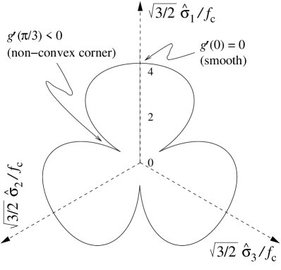
(a) (b)

Figure 9: An example of non-convex yield surface, corresponding to eqns. (A.10), satisfying the Laydi and Lexcellent (2009) conditions (A.8). (a) Deviatoric section. (b) Yield surface in the biaxial plane $\sigma_{1}/f_{t}$ vs. $\sigma_{2}/f_{t}$, with $\sigma_{3}=0$.

References

- [1] Babua, R.R., Benipal, G.S. and Singh, A.K. (2005) Constitutive modelling of concrete: an overview. Asian J. Civil Eng. (Building and Housing) 6, 211-246.
- [2] Bai, Y. and Wierzbicki, T. (2008) A new model of metal plasticity and fracture with pressure and Lode dependence. Int. J. Plasticity 24, 1071-1096.
- [3] Bigoni, D. and Piccolroaz, A. (2004) Yield criteria for quasibrittle and frictional materials. Int. J. Solids Struct. 41, 2855-2878.
- [4] Coppola, T and Folgarait, P. (2007) The influence of stress invariants on ductile fracture strain in steels. (in Italian) Proc. XXXVI AIAS Congress, Sept. 4-8, 2007.
- [5] Dal Maso, G., Demyanov, A. and DeSimone, A. (2007) Quasistatic Evolution Problems for Pressure-sensitive Plastic Materials. Milan J. Math. 75, 117-134.
- [6] Descamps, F. and Tshibangu, J.P. (2007) Modelling the Limiting Envelopes of Rocks in the Octahedral Plane. Oil & Gas Science and Technology - Rev. IFP, 62, 683-694.
- [7] DorMohammadi, H. and Khoei, A.R. (2008) A three-invariant cap model with isotropic?kinematic hardening rule and associated plasticity for granular materials. Int. J. Solids Struct. 45, 631-656.
- [8] Hartmann, S. and Bier, W. (2008) High-order time integration applied to metal powder plasticity. Int. J. Plasticity 24, 17-54.
- [9] Heisserer, U., Hartmann, S., Düster, A., Bier, W., Yosibash, Z. and Rank, E. (2008) p-FEM for finite deformation powder compaction. Comput. Method. Appl. M. 197, 727-740.
- [10] Hill, R. (1950) Inhomogeneous Deformation of a Plastic Lamina in a Compression Test. Phil. Mag. 41, 733-744.
- [11] Hill, R. (1968) On constitutive inequalities for simple materials-I. J. Mech. Phys. Solids 16, 229-242.
- [12] Hill, R. (1970) Constitutive inequalities for isotropic elastic solids under finite strain. Proc. R. Soc. Lond. 314, 457-472.
- [13] Hu, W. and Wang, Z.R. (2005) Multiple-factor dependence of the yielding behavior to isotropic ductile materials. Comput. Mat. Sci. 32, 31-46.
- [14] Laydi, M.R and Lexcellent, C. (2009) Yield criteria for shape memory materials: convexity conditions and surface transport. Math. Mech. Solids doi:10.1177/1081286508095324.
- [15] Lavernhe-Taillard, K., Calloch, S., Arbab-Chirani, S. and Lexcellent, C. (2009) Multiaxial Shape Memory Effect and Superelasticity. Strain 45, 77-84.
- [16] Neale, K.W. (1981) Phenomenological constitutive laws in finite plasticity. SM Archives 6, 79-128.
- [17] Ogden, R.W. (1982) Elastic deformations of rubberlike solids. In Mechanics of Solids, The Rodney Hill 60th Anniversary Volume (Eds. H.G. Hopkins and M.J. Sewell), Pergamon Press, pp. 499-537.
- [18] Ogden, R.W. (1984) Non-linear elastic deformations. Chichester, Ellis Horwood.
- [19] Raniecki, B. and Mróz, Z. (2008) Yield ormartensitic phase transformation conditions and dissipation functions for isotropic, pressure-insensitive alloys exhibiting SD effect. Acta Mech. 195, 81-102.
- [20] Saint-Sulpice, L., Arbab Chirani, S. and Calloch, S. (2009) A 3D super-elastic model for shape memory alloys taking into account progressive strain under cyclic loadings. Mech. Materials 41, 12-26.
- [21] Sheldon, H.A., Barnicoat, A.C. and Ord, A. (2006) Numerical modelling of faulting and fluid flow in porous rocks: An approach based on critical state soil mechanics. J. Struct. Geol. 28, 1468-1482.
- [22] Taillard, K., Arbab Chirani, S. Calloch, S. and Lexcellent, C. (2008) Equivalent transformation strain and its relation with martensite volume fraction for isotropic and anisotropic shape memory alloys. Mech. Materials 40, 151-170.
- [23] van Tiel, J. (1984) Convex Analysis. Wiley & Sons, Chichester.
- [24] Valoroso, N. and Rosati, L. (2009) Consistent derivation of the constitutive algorithm for plane stress isotropic plasticity. Part II: Computational issues. Int. J. Solids Struct. 46, 92-124.
- [25] Yang, W.H. (1980) A useful theorem for constructing convex yield functions. ASME J. Appl. Mech. 47, 301-303.
- [26] Wierzbicki, T., Bao, Y., Lee, Y-W., Bai, Y. (2005) Calibration and evaluation of seven fracture models. Int. J. Mech. Sci. 47, 719-743.