The normal field instability under side-wall effects: comparison of experiments and computations

Abstract

We consider a single spike of ferrofluid, arising in a small cylindrical container, when a vertically oriented magnetic field is applied. The height of the spike as well as the surface topography is measured experimentally by two different technologies and calculated numerically using the finite element method. As a consequence of the finite size of the container, the numerics uncovers an imperfect bifurcation to a single spike solution, which is forward. This is in contrast to the standard transcritical bifurcation to hexagons, common for rotational symmetric systems with broken up-down symmetry. The numerical findings are corroborated in the experiments. The small hysteresis observed is explained in terms of a hysteretic wetting of the side wall.

1 Introduction

Rotational symmetric systems with broken up-down symmetry become first unstable due to a transcritical bifurcation to hexagons, which is hysteretic  [cross1993]. Examples are non-Boussinesq Rayleigh-Bènard convection [busse1967] and chemical reactions of the Turing type [turing1952]. The same is true, when a layer of magnetic fluid is exposed to a normal magnetic field. Above a certain critical induction $B_{c}$, a hexagonal pattern of liquid spikes appears on the surface of the fluid. This striking phenomenon was first reported by cowley1967 and described in terms of a linear stability analysis. This observation $40$ years ago triggered numerous efforts to describe also the nonlinear aspects of the phenomenon theoretically. gailitis1977, later friedrichs2001 and friedrichs2002 and most recently bohlius2006b used the principle of free energy minimisation to predict the pattern ordering, wavelength and final amplitude of the peaks on an infinitely extended surface. The numerical computations by boudouvis1987phd and boudouvis1987 specify quantitatively the hysteresis in spike height in unbounded ferrofluid pools. matthies2005 calculate also the dynamics of an infinite periodic lattice of peaks.

The experiments, however, are performed with limited amounts of fluid. A finite layer depth in the vertical dimension has been incorporated into the theory by friedrichs2001. According to lange2000, the infinitely deep limit is well approximated if the depth exceeds at least the wavelength of the pattern. However, in the horizontal dimension the finite container size has not been considered. Therefore, experimental realizations approximated this limit of an infinitely extended layer by several different approaches. abou2001 used a very large aspect ratio, whereas gollwitzer2007 employed an inclined container edge. richter2005 used a magnetic ramp to minimize the influence of the border for the Rosensweig instability, whereas embs2007 independently applied it to the Faraday instability in ferrofluid.

The question arises, what happens if the container size is intentionally reduced until only a single spike is left. In this case, all symmetries are kept, nonetheless the character of the bifurcation may change. Indeed, in experiments before the seminal work of bacri1984, it was difficult to uncover a hysteresis due to the small container size.

Although there have been numerous experiments in small containers merely because they are simple and cheap, a systematic study of the influence of the constrained geometry on the bifurcation is missing. One reason is, that model descriptions which deal with the finite container size are rare. So far, we know only the work by friedrichs2000 where the free surface is modeled by a four parameter function to fit the measurements by mahr1998. In this case, a highly susceptible fluid still showed a hysteretic transition.

In the present article, we demonstrate, that a transcritical bifurcation to hexagons, as found by gollwitzer2007, e.g., becomes an imperfect supercritical bifurcation to a single spike if the container size is reduced sufficiently. This is the outcome of a numerical model which is able to calculate the stable and unstable solutions for given container size and fluid parameters. It also takes into account the side-wall effects, namely the wetting and the fringing field. We compare the numerical results with our measurements of the surface topography. For the first time, we apply two different techniques which are capable of recording the amplitude [megalios2005] and also the full topography of the fluid surface [richter2001], to the same experiment.

In the following two sections, we give an overview over the experimental methods. Subsequently, we describe the numerical computations. Finally, we compare all three results.

2 Measurements of the material properties

Quantity		Value $\pm$	Error
Surface tension	$\sigma$	$30.57\ \pm$	$0.1\,\mathrm{mN\,m^{-1}}$
Density	$\rho$	$1236\ \pm$	$1\,\mathrm{kg\,m^{-3}}$
Contact angle with the container wall	$\theta_{c}$	$10\pm 0.3$ °
Viscosity	$\eta$	$120\ \pm$	$5\,\mathrm{mPa\,s}$
Saturation magnetization	$M_{S}$	$28.7\ \pm$	$0.1\,\mathrm{kA\,m^{-1}}$
Initial susceptibility	$\chi_{0}$	$1.2023\ \pm$	$0.005$

Table 1: Material properties of the ferrofluid APG 512a (Lot F083094CX) from Ferrotec Co.

We used the ferrofluid APG 512a (Lot F083094CX) from Ferrotec for all experiments. It is based on an ester with a very low vapor pressure, suitable for vacuum pumps. It has an excellent long-term stability. Over one year, the critical induction has not changed by more than $3\,\%$. In contrast to less stable magnetic liquids, the formation of agglomerates in the tips of the Rosensweig spikes was not observed. After applying magnetic fields for an hour, the field was switched off. Neither the visual inspection nor the X-ray images unveiled any agglomerates at the site of the spikes.

The Rosensweig instability is a counterplay between gravitational and surface terms on the one hand and magnetic forces on the other hand [cowley1967]. Therefore, a set of basic material properties of the fluid is necessary for a comparison with the theory, namely the surface tension $\sigma$, the density $\rho$ and the magnetization curve $M(H)$. These quantities are summarized in table 1.

The surface tension has been measured using a commercial ring tensiometer (LAUDA TE1). This device wets a ring made from platinum wire, pulls it off the fluid surface and determines the maximum force acting on the ring, from which the surface tension can be computed following dunouy1919. According to an analyis by harkins1930, the error for this method is smaller than $0.25\,\%$, given that the density of the fluid and the geometry of the ring are known with sufficient accuracy.

The density $\rho$ has been measured using a commercial vibrating-tube densimeter (DMA 4100 by Anton Paar). This device enables us to determine the density with an error of $0.01\,\%$.

The contact angle $\theta_{c}$ was determined with the contact angle system OCA 20 (Dataphysics) by optical means. Three measurements were performed at the inner side wall of the container, which was tilted by $90\,$°. The difference between advancing and receding angle could not be measured in this way.

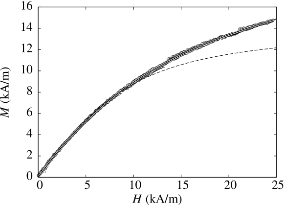
Figure 1: The magnetization curve of the ferrofluid. The circles denote the experimental values, the solid line is a fit with the model by ivanov2001. The dashed line is a fit with the Langevin function, that is valid only up to $H\lessapprox 10\,\mathrm{kA/m}$.

The magnetization curve $M(H)$ of the ferrofluid has the biggest influence on the surface pattern. It has been meticulously measured using a fluxmetric magnetometer consisting of a Helmholtz pair of sensing coils with $6800$ windings and a commercial integrator (Lakeshore Fluxmeter 480). The sample has been held in a spherical cavity with a diameter of $12.4\,\mathrm{mm}$. This spherical shape ensures a homogeneous magnetic field inside the sample and an exact homogeneous demagnetization factor of $1/3$, which makes it possible to get accurate results over the whole range of $H$. Figure 1 shows the magnetization curve of our ferrofluid. The solid and the dashed line provide two analytic approximations to $M(H)$. The dashed line is a fit with the Langevin approximation for monodisperse colloidal suspensions and provides the constitutive equation [rosensweig1985]

$$\left|\underline{M}\right|=p\left[\coth\left(\tau\left|\underline{H}\right|\right)-\frac{1}{\tau\left|\underline{H}\right|}\right].$$ (1)

Only the data points within a range of $H\in[0\dots 10\,\mathrm{kA/m}]$ have been taken into account for the estimation of the adjustable parameters $p=14.6\,\mathrm{kA/m}$ and $\tau=0.24\,\mathrm{m/kA}$. A satisfying fit of the whole curve with this equation is not possible, because real ferrofluids consist of magnetic particles with a broad size distribution [popplewell1995b]. We therefore make use of a model for dense polydisperse magnetic fluids put forward by ivanov2001. The solid line in figure 1 displays the best fit with that model. The saturation magnetization given in table 1 is extrapolated from there. This extrapolation indicates together with the manufacturer information $M_{S}\approx 26\,$kA/m$\pm 10\,\%$, that this model is very well fitted to our dense ferrofluid ivanov2007cf..

3 Measurements of the surface pattern

We fill a cylindrical container, machined from aluminum, with the ferrofluid and expose it to a magnetic induction ranging from $B=7.6\,\mathrm{mT}$ to $B=37.7\,\mathrm{mT}$. The depth of the container amounts to $20\,\mathrm{mm}$ and the diameter is $29.7\,\mathrm{mm}$. This diameter is chosen by trial such that only one single spike emerges in the centre of the vessel for all magnetic inductions we apply. From the weight of the filled container and the density, we calculate the amount of ferrofluid filled into the container to $V_{0}=6.387\,\mathrm{ml}$, which is equivalent to a filling height of $D=9.22\,\mathrm{mm}$. Two complementary experimental methods were used to determine the height of the emerging spike in the centre of the vessel: the X-ray method by richter2001 and the laser method by megalios2005, which are described in the following.

3.1 X-ray method

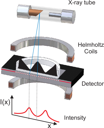
Figure 2: The experimental setup for the X-ray method by richter2001

.

The X-ray apparatus comprises a stable X-ray point source, that emits radiation vertically from above through the fluid layer. The container is placed midway between a water cooled Helmholtz pair of coils, which generate a DC magnetic field of up to $40\,\mathrm{mT}$. Directly below the container an X-ray camera with $512\times 512$ pixels is located, which measures the transmitted intensity at every pixel in one plane underneath the fluid [richter2001]. This setup is depicted in figure 2. The transmitted intensity of the X-rays is directly related to the height of the fluid above every corresponding pixel. To calibrate this relation, we use a wedge of known size, fill it with ferrofluid and place it in the empty container. In this calibration image, we therefore know the height of the fluid. Figure 3 shows the calibration data from the wedge. These are then fitted with an overlay of three exponential functions

$$I(h)=I_{0}\cdot\sum\limits_{i=1}^{3}\alpha_{i}\exp(-\beta_{i}h)$$ (2)

as a practical approximation, denoted by the solid line in figure 3. Further details can be found in gollwitzer2007.

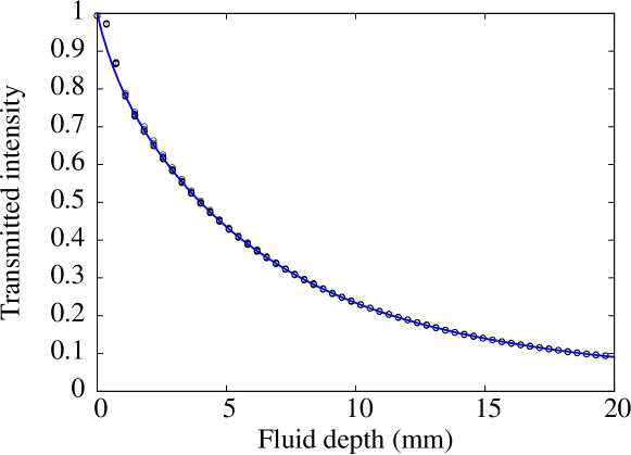
Figure 3: The transmitted intensity as a function of the fluid depth. The solid line is a fit with equation (2).

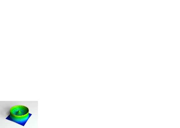
Figure 4: Three-dimensional reconstruction of the surface of the single spike at an induction of $B=22.69\,\mathrm{mT}$. A related movie can be accessed here.

After applying the inverse of (2) to an arbitrary image from the detector, we finally end up with a complete three-dimensional surface topography of the filled container. A reconstruction for one specific field is displayed in figure 4. A survey of the surface topography for different fields is provided by the related movie.

3.2 Laser method

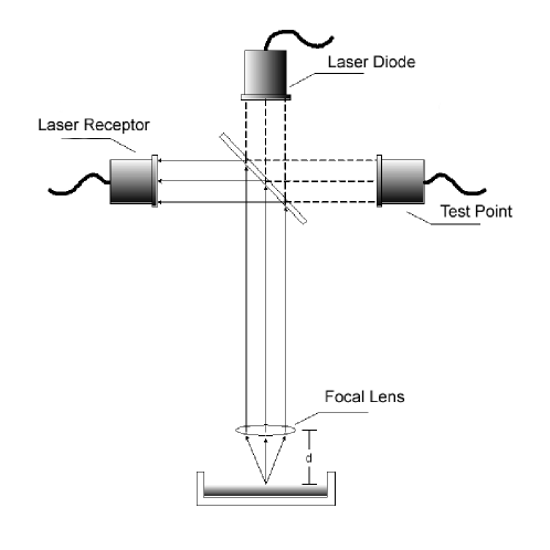
Figure 5: The experimental setup of the laser method by megalios2005. The solid lines denote the path of the light reflected on the surface. The path sketched by the dashed lines is used to verify that the laser operates.

The laser method developed by megalios2005 enables precise, relative measurements of the extrema of the surface topography. Figure 5 depicts the principle of operation. The container with the ferrofluid is situated in a long solenoid, which generates a vertical magnetic field. The solenoid is $33\,\mathrm{cm}$ long with an internal diameter of $13\,\mathrm{cm}$ and an external diameter of $14\,\mathrm{cm}$. It has $1124$ windings and produces up to $21\,\mathrm{mT}$ at its centre, with a variation of less than $1\,\%$ at the experimental region.

A laser beam is directed at the fluid surface through a semitransparent mirror, which splits the beam into two parts. One part is deflected sideways onto a test point and serves as an indicator, whether the laser operates correctly (the dashed path in figure 5). The other beam is focused on the fluid surface and the reflected light is deflected by the semitransparent mirror onto a photodiode detector (the solid path in figure 5).

The position of the focal spot can be adjusted by means of a micrometre screw. The maximum of the reflected intensity is reached, when the direction of the beam coincides with the normal vector of the surface at the focus spot and the distance of the lens from the surface is equal to the focal length. In normal operation, the beam is oriented vertically - thus the intensity of the signal reaches its maximum when the focus spot hits an extreme point of the surface, namely the top of a spike or the minimum in the centre of the meniscus. By tracing the maximum intensity of the reflected beam and recording the position of the laser optics, we get the position of the spike with micrometre resolution relative to some reference point. Also the absolute height of the spike above the bottom of the container can be determined by setting the reference point at the top of the container edge.

4 Governing equations and computational analysis

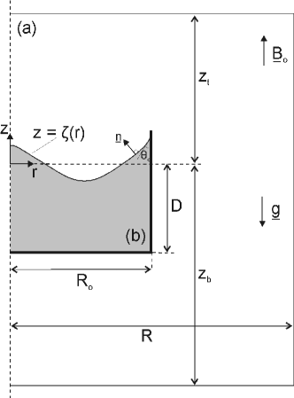
Figure 6: A small axisymmetric ferrofluid pool in the magnetic field.

A scheme of a small cylindrical ferrofluid pool in a vertical magnetic field is shown in figure 6. The surrounding air and the embedded ferrofluid are denoted by (a) and (b), respectively. The applied field can be produced either by a pair of Helmholtz coils or a solenoid of suitable dimensions. It is uniform i. e., of constant strength and vertical orientation, in a region far away from the pool. The field uniformity, however, is disturbed in the neighborhood of the pool, due to the demagnetizing field of the pool itself. Therefore, the applied magnetic field could be taken uniform only away from the pool. In the following, the magnetic field distribution and the free surface deformation are taken as axially symmetric about the $r=0$ axis (cf. figure 6).

The field distribution in regions (a) and (b) is governed by the equations of magnetostatics. The Gauss law for the magnetization reads

$$\nabla\cdot\underline{B}=0,$$ (3)

where $\underline{B}$ is the magnetic induction. Since the magnetic field $\underline{H}$ is irrotational it can be derived from a magnetostatic potential $\underline{H}\equiv\nabla u$ both inside and outside the ferrofluid and, provided that the materials are isotropic, it is parallel to $\underline{B}$ and so is the magnetization

$$\underline{B}=\mu\underline{H}=\mu_{0}(\underline{H}+\underline{M}).$$ (4)

The magnetic permeability $\mu$ is constant in non-magnetic media, namely $\mu_{\text{a}}=\mu_{0}=4\pi\times 10^{-7}\mathrm{H/m}$; inside the ferrofluid, it depends on the field. Two different constitutive equations are used to account for the field dependence on the magnetization. The first one comes from Langevin’s theory for monodisperse colloidal suspensions (equation 1). The second one comes from a polydisperse model by ivanov2001 that is based on the assumption of a gamma distribution of particle diameters.

Writing equation (3) in terms of the magnetostatic potential, $u$, and taking into account the equation (4) yields

$$\nabla^{2}u_{\text{a}}=0,\quad\nabla\cdot(\mu\nabla u_{\text{b}})=0$$ (5a,b)

inside the non-magnetic phase (a) and inside the magnetic phase (b), respectively.

Equlibrium is governed by force balance along the ferrofluid free surface which is stated by the magnetically augmented Young-Laplace equation of capillarity

$$-g\Delta\rho\zeta+\frac{1}{2}\mu_{0}\int\limits_{0}^{H_{\text{bs}}}M(H^{\prime})\mathrm{d}H^{\prime}+2\aleph\sigma=K,\text{at }z=\zeta(r),\quad 0\leq r\leq R_{0}$$ (6)

where $g$ is the gravitational acceleration, $\rho$ is the density, $\sigma$ is the surface tension and $\zeta$ is the vertical displacement of the free surface parametrized by the radial coordinate $r$, i.e., $\zeta=\zeta(r)$. The upper limit $H_{\text{bs}}$ of the integral in the magnetization term is the field strength in the ferrofluid, evaluated at the free surface, i.e. at $z=\zeta(r).$

The reference pressure $K$ is constant at the free surface. The unit normal to the free surface $\underline{n}$ and the local mean curvature of the free surface $2\aleph$ are

$$\underline{n}=\frac{-\zeta_{r}\underline{e}_{r}+\underline{e}_{z}}{\sqrt{1+\zeta_{r}^{2}}},\quad 2\aleph=\frac{1}{r}\frac{\mathrm{d}}{\mathrm{d}r}\left(\frac{r\zeta_{r}}{\sqrt{1+\zeta_{r}^{2}}}\right),$$ (7a,b)

where $\underline{e}_{r}$ and $\underline{e}_{z}$ are mutually orthogonal unit vectors along the $r$- and $z$-axis, respectively, and $\zeta_{r}\equiv\mathrm{d}\zeta/\mathrm{d}r$.

The reference pressure $K$ in equation (6) is determined by the constraint, that the ferrofluid volume is of fixed amount

$$2\pi\int\limits_{0}^{R_{0}}\zeta r\mathrm{d}r=C=\text{const},$$ (8)

i.e. we assume an incompressible liquid. The coordinate system, i.e. the location of the $z=0$ line, is chosen such that $C=0$.

The set of the governing equations (5a,b), (6) and (8), needs to be solved for the magnetostatic potential $u_{a}(r,z)$ and $u_{b}(r,z)$, the free surface shape $\zeta(r)$ and the reference pressure $K$, taking into account the following boundary conditions (see also figure 6):

$$\frac{\partial u_{\text{a}}}{\partial r}=\frac{\partial u_{\text{b}}}{\partial r}=0,\quad\zeta_{r}=0\text{ at }r=0$$ (9)

$$u_{\text{a}}=u_{\text{b}},\quad\mu\underline{n}\cdot\nabla u_{\text{b}}=\mu_{0}\underline{n}\cdot\nabla u_{\text{a}}\quad\text{ at }z=\zeta(r)\text{ and }0\leq r\leq R_{0}$$ (10)

$$u_{\text{a}}=u_{\text{b}},\quad\mu\frac{\partial u_{\text{b}}}{\partial r}=\mu_{0}\frac{\partial u_{\text{a}}}{\partial r}\quad\text{ at }r=R_{0}\text{ and }-D\leq z\leq\zeta(R_{0})$$ (10)

$$u_{\text{a}}=u_{\text{b}},\quad\mu\frac{\partial u_{\text{b}}}{\partial z}=\mu_{0}\frac{\partial u_{\text{a}}}{\partial z}\quad\text{ at }z=-D,0\leq r\leq R_{0}$$ (10)

$$u_{\text{a}}=0\text{ at }z=-z_{\text{b}}$$ (11)

$$\frac{\partial u_{\text{a}}}{\partial z}=\frac{B_{0}}{\mu_{0}}\text{ at }z=z_{t},\quad\frac{\partial u_{\text{a}}}{\partial r}=0\text{ at }r=R$$ (12)

$$\zeta_{r}=\cot\theta_{c}\text{ at }r=R_{0}.$$ (13)

The subscripts $r$ and $z$ denote differentiation with respect to $r$ and $z$, respectively. Equations (9) are the conditions that the shape of the free surface and the magnetostatic potential are axially symmetric. Equations (10) are statements of the continuity of the potential and of the normal component of the magnetic induction across interfaces between two media with different magnetic permeabilities. A datum for the potential is fixed by (11). Equations (12) are the conditions that the magnetic field be uniform far away from the pool. A contact angle $\theta_{c}$ is prescribed by equation (13) and reflects the wetting properties of the magnetic liquid in contact with the solid wall of the container.

The governing equations give rise to a nonlinear, free boundary problem, owing to the presence of the free surface, the location of which enters the equations nonlinearly and is unknown a priori. An additional nonlinearity comes from the constitutive equation for the magnetization of the fluid. Such a problem is only amenable to computer-aided solution methods. The choice is the combination of Galerkin’s method of weighted residuals and finite element basis functions [kistler1983].

Figure 7: Sample of the discretized domain

Here we will only outline the application of the method. Details can be found in previous works by boudouvis1988 and papathanasiou1998. The domain is tessellated into nine-node quadrilateral elements between vertical spines and transverse curves whose intersections with each spine are located at distances that are proportional to the displacement of the interface along that spine. The tessellation creates a mesh of nodes and at each node a finite element basis function is assigned that is unity at that node and zero at all other nodes. As the basis functions, we choose a quadratic polynomials of the independent variables $r$ and $z$. A sample of the computational mesh is shown in Figure 7. The dependent variables $u_{\text{a}}(r,z),u_{\text{b}}(r,z)$ and $\zeta(r)$ are approximated in terms of a truncated set of the finite element basis functions. The governing equations are reduced with Galerkin’s method to a set of nonlinear algebraic equations for the values of the unknowns $u_{\text{a}},u_{\text{b}}$ and $\zeta$ at the nodes and for the value of $K$.

At fixed values of the physical parameters, the nonlinear algebraic equation set is solved by Newton iteration. The parameter of interest here is the applied magnetic induction $B_{0}$, which appears in the boundary conditions (cf. equation 12a). Solution families, i.e., solutions at sequences of different values of $B_{0}$ are systematically traced with first-order continuation. The computational results reported are obtained with a mesh of 24000 nodes. The sensitivity of the spike height to further mesh refinement is practically negligible; namely, less than 0.2 % when doubling the mesh density. Three to five Newton steps are needed for the convergence at each value of the continuation parameter.

5 Comparison of experimental and numerical results

We record the surface profile for $200$ different magnetic inductions $B_{0}\in\left[7.6\,\mathrm{mT}\dots 37.7\,\mathrm{mT}\right]$ with the X-ray method described above. Unevitably, the magnetic induction in the neighborhood of the container is distorted and emphasized in comparison to the induction for empty coils. The given values $B_{0}$ denote the spatially averaged magnetic induction below the container at a vertical distance of $23.8\,\mathrm{mm}$ from the bottom of the fluid layer. This corresponds to the boundary of the computational domain in the calculations. The height and position of the extreme point of the surface topography in the centre has been determined by fitting a paraboloid to a small circular region of the surface with a diameter of $1.5\,\mathrm{mm}$. Figure 8 shows the resulting central height $\hat{h}(B_{0})$. The red solid line marks the data for increasing induction. The magnetic fluid first rises at the edge of the container, thus the level of fluid in the centre of the vessel drops. The central height then corresponds to the minimum level in the centre. At a magnetic induction of around $16\,\mathrm{mT}$, a single spike emerges in the centre that continues to rise for increasing induction. The central height then corresponds to the height of this spike. A small hysteresis is found when decreasing the field again. See the blue line in figure 8.

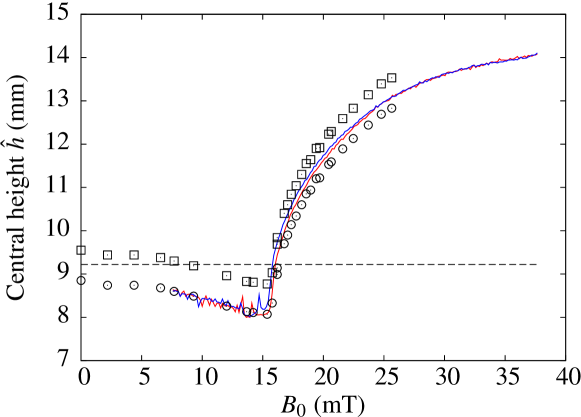
Figure 8: Height of the single spike or the minimum in the centre, respectively. The numbers given are the total absolute height of the fluid above the bottom of the container. For clarity, the individual 200 data points for one sweep are connected by a solid line. The red (blue) line denotes the values from the X-ray measurement for increasing (decreasing) field, respectively. The open squares show the result of the laser measurement. The open circles denote the laser data shifted on top of the X-ray data. The dashed line represents the filling level of the fluid according to the weight, neglecting the effects of the meniscus.

Using the laser method, we performed measurements of the spike height for $29$ different magnetic inductions from $0$ to $25.65\,\mathrm{mT}$, which are also plotted in figure 8. By focusing the laser beam on top of the container edge, a reference point was taken to get absolute values for the central height $\hat{h}$ above the bottom of the container, denoted by the open squares. They differ from the X-ray measurement by a shift of $0.7\,\mathrm{mm}$. However, if the reference point is adjusted by this shift, we find a nice coincidence of the data points from both methods, as shown by the open circles in figure 8.

The inaccuracy of the reference point of the laser method can well be explained from the fact, that the laser beam cannot be focused precisely onto the top edge of the container. The vessel is machined from aluminum with a quite rough surface and diffuses the incident laser beam, which leads to the observed shift. This has been experimentally verified by comparing the height measurements of the bare aluminium and a ferrofluid surface at the same level. The difference in the reading is large enough to explain the shift between the laser data and the X-ray data. On the other hand, the accuracy of the reference point of the X-ray measurement depends on the positioning of the calibration wedge. The resolution of this position is limited by the lateral resolution of the detector, which leads to an estimate of the absolute error of $0.2\,\mathrm{mm}$. Due to the roughness of the aluminium vessel, the X-ray data seem to be more precise than the laser data concerning the absolute height in the present experiment. Relatively, both yield practically the same result.

Further deviations may stem from the different ambient temperature at which the data were taken. Whereas in Bayreuth, the lab temperature was stabilized at $21\,\pm 1$ °C, the temperature in Athens was $30\,$°C. This leads to a reduced magnetisation and may be the origin of a reduced spike height for higher fields (cf. figure 8).

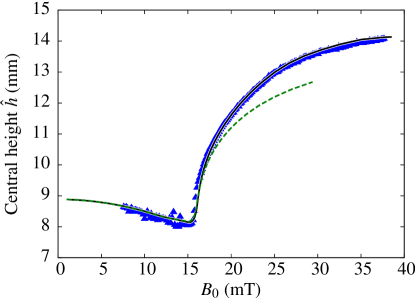
(a)

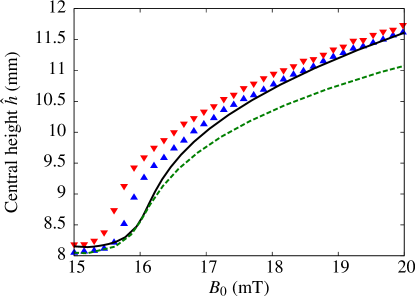
(b)

Figure 9: The central height $\hat{h}$ from the computations (lines) and from the X-ray experiment (triangles). Blue upward (red downward) triangles denote the values for increasing (decreasing) induction, respectively. The dashed green line is based on Langevin’s law for the magnetisation, while the black solid line employs ivanov2001 model. (a) Full range (b) Zoom

After successfully comparing the results of the two measurement techniques, we now present the numerical predictions. The results of the computational analysis are depicted in figure 9 together with the X-ray data. The value corresponding to the central height $\hat{h}$ of the measurements is the height at the axis of symmetry $\left.h\right|_{r=0}=\left.\zeta\right|_{r=0}+D$, where $D$ denotes the filling level. Two computational equilibrium paths are shown for two different models for the magnetziation $M(H)$. The green dashed line displays the numerical result using Langevin’s equation (1), while the black line makes use of the model by ivanov2001. For magnetic inductions up to $17\,\mathrm{mT}$ there is no noticable difference between both results. This is explained by the coincidence of both magnetization laws up to an internal field of $H\approx 10\,\mathrm{kA/m}$, as shown in figure 1. For higher fields, however, Langevin’s law is no longer valid. This leads to a rather big deviation between both theoretical curves. Regardless of the underlying magnetisation curve, the numerical solutions show a continuous behaviour of $\hat{h}$ in the full range of $B_{0}$. In particular, no turning points are traced on the curve. This is mentioned, since a pair of turning points, if existed, should imply a hysteresis in surface deformation observed when increasing and then decreasing $B_{0}$. Thus, from the theoretical calculations we do not expect any hysteresis. We stress this fact, because in the case of an infinitely extended container, a hysteresis is both expected theoretically [e.g.]friedrichs2001cf. and found in the experiment and numerical calculations [e.g.]gollwitzer2007. Moreover, we tested the influence of the contact angle. A computation for $\theta_{c}=20\,$°does not deviate more than $60\,\upmu\mathrm{m}$ from the above calculation over the full range of $B$. Thus, the spike height does only weakly depend on the contact angle.

Next, we compare the measurements with the numerical results. In the full range, the experimental data coincide very well with the more advanced computations taking into account the magnetization law by ivanov2001. The difference is within only $1\,\%$ of the absolute height, except near the threshold, where it amounts to $6\,\%$. This is natural for a sigmoidal function, where close to the steep increase the error can become arbitrarily large, when there are unertainties of the control parameter. The difference between the thresholds in theory and experiment amounts to at most $3\,\%$ as can be seen from Figure 9 (b). It shows an enlarged view of $\hat{h}$ in the immediate vicinity of the threshold. In opposite to the numerical results, we observe in the experiment a small hysteresis between the data for increasing $B_{0}$, as marked by upwards triangles, and the one for decreasing $B_{0}$, denoted by downward triangles. The hysteresis is in the range of $\Delta B_{0}=0.2\,$mT. The origin for this hysteresis is a priori not clear.

Note, that gollwitzer2007, e.g., measure a hysteresis of $\Delta B^{\mathrm{\infty}}=0.17\,$mT for the same ferrofluid as in our case in a container with a diameter of $\approx 10\times\lambda_{c}$. Remarkably, this value is in the same range as the one observed above. If the hysteresis in our experiment would be of the same nature, it should be much smaller due to the imperfection caused by the container edge [cross1993]. Therefore we suspect another mechanism. One candidate is a hysteretical wetting of the cylindrical wall. The difference between the advancing and the receding contact angle can be as large as $10\,$° for a surface that has not been specially prepared [degennes1985, dussan1979]. Moving the contact line always costs energy. This may explain the small hysteresis of the spike height for increasing and decreasing induction. In our experiment, this effect is important, because the interfacial area between the fluid and the vertical wall is comparable to the free surface of the fluid.

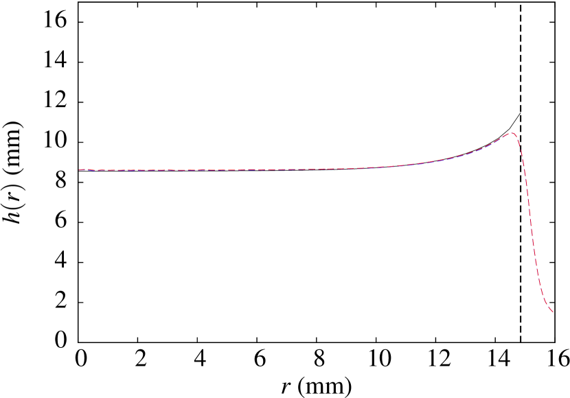
(a)

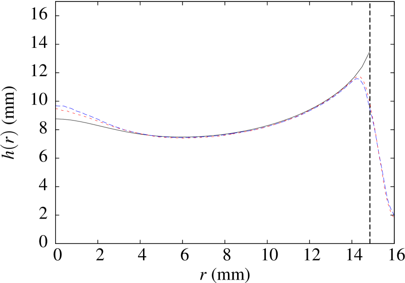
(b)

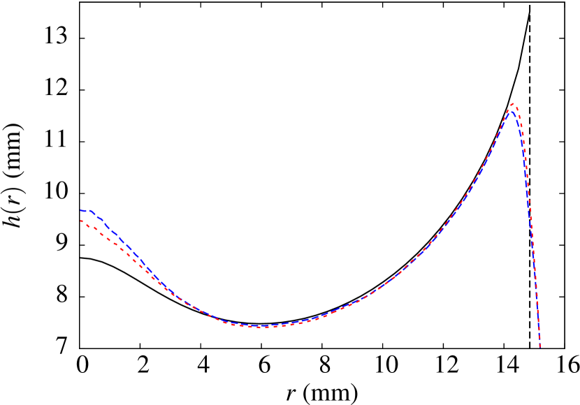
(c)

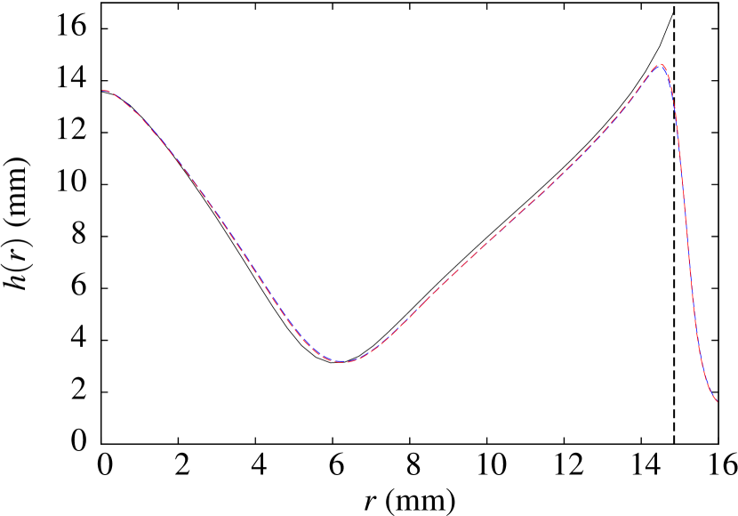
(d)

Figure 10: The ferrofluid free surface shapes at various magnetic field strengths. The solid lines show the numerically computed profiles, while the red (blue) dashed line gives radial interpolation of the experimental data for increasing (decreasing) magnetic induction. The vertical dashed line shows the side wall of the container. (a) $B=7.39\,\mathrm{mT}$, (b) $B=16.17\,\mathrm{mT}$, (c) Zoom of (b), (d) $B=29.70\,\mathrm{mT}$

The availability of the complete surface topography from the X-ray method allows us not only to compare the central height, but also the shape of the spike or meniscus, respectively. Examples for the free surface shapes at selected values of the magnetic induction are shown in figure 10. The experimental data have been averaged angularly around the centre of the observed spike, which is not exactly in the centre of the container in the experiment. This off-centre distance is rather small ($0.05\,\mathrm{mm}$), however it must be taken into account, otherwise the averaging would disturb the shape of the spike.

Similiarly to the comparison of the height alone, there are only slight differences between the computations and the experimentally observed shape. Most notably, we discern a drop at the edge of the container. The reason for this difference is two-fold: first, the angular average does not work well near the container border, because the centre of the spike is off-axis, as explained before. Second, the X-ray method has problems to accurately detect the height near the border, where the container wall shadows the X-rays. Further, for magnetic inductions near the threshold (cf. figure 10 (b) and (c)), the height of the tip differs by $\approx 1\,\mathrm{mm}$. The reason is probably a slight shift of the critical induction (cf. figure 9), where the height is very sensitive to small changes of the induction $B$.

The hysteresis, already observed from the central height alone, manifests itself by a difference of the surface profiles for increasing and decreasing induction. Far away from the threshold, both profiles match nearly perfectly (figure 10 (a) and (d)), while there is a clear difference near the threshold (figure 10 (b) and (c)). The tip of the spike is considerably smaller for an increasing magnetic induction, while the level of the fluid near the container edge is higher. This corroborates a hysteretical wetting to be responsible for the hysteresis.

Apart from these differences, the deviation between the computed and measured profiles is around $1\,\%$.

6 Discussion and Conclusion

For a rotational symmetric system with broken up-down symmetry we have reduced the container size until only a single entity remains. In the case of the Rosensweig instability this is a single spike of ferrofluid. Whereas for our fluid, the extended system exhibits a transcritical bifurcation to hexagons, here an imperfect bifurcation sets in, and the axisymmetric free surface deformation evolves supercritically and monotonically. This is at least the outcome of the monolithic finite element approach, which takes into account the side-wall effects, namely the wetting and the fringing field, as well as the polydispersity of the fluid. We find a convincing agreement between theory and two independent measurement techniques, the errors being within $3\,\%$ without any adjustable parameter. The nonetheless observed hysteresis is due to the wetting.

Our findings immediately raise the issue of what is “in between”, regarding the structure of the solution space – that is surface deformation versus applied field and other key parameters – as the size of the pool grows laterally. This will be tackled in a forthcoming publication by spyropoulos2006.

A transition from a transcritical backward to an imperfect forward bifurcation under spatial constraints has also been reported by peter2005shc. Their spatial stripe forcing simultaneously breaks the rotational and translational symmetry. In our case it is sufficient to break the translational symmetry.

To conclude, we have quantitatively compared numerics and experiments of the Rosensweig instability in a system of finite size. This is a specific example, how external constraints may change a perfect transcritical bifurcation to an imperfect supercritical one.

References

References

- [1] \harvarditemAbou et al.2001abou2001 Abou B, Wesfreid J E \harvardand Roux S 2001 J. Fluid. Mech. 416, 217–237.
- [2] \harvarditemBacri \harvardand Salin1984bacri1984 Bacri J C \harvardand Salin D 1984 J. Phys. Lett. (France) 45, L559–L564.
- [3] \harvarditemBohlius et al.2006bohlius2006b Bohlius S, Pleiner H \harvardand Brand H 2006 J. Phys.: Condens. Matter. 18, 2671–2684.
- [4] \harvarditemBoudouvis1987boudouvis1987phd Boudouvis A G 1987 Mechanisms of Surface Instabilities and Pattern Formation in Ferromagnetic Liquids PhD thesis University of Minnesota Minneapolis, MN, USA.
- [5] \harvarditemBoudouvis et al.1988boudouvis1988 Boudouvis A G, Puchalla J L \harvardand Scriven L E 1988 Chem. Eng. Comm. 67(1), 129–144.
- [6] \harvarditemBoudouvis et al.1987boudouvis1987 Boudouvis A G, Puchalla J L, Scriven L E \harvardand Rosensweig R E 1987 J. Magn. Magn. Mater. 65, 307–310.
- [7] \harvarditemBusse1962busse1967 Busse F H 1962 J. Fluid Mech. 30, 625–649.
- [8] \harvarditemCowley \harvardand Rosensweig1967cowley1967 Cowley M D \harvardand Rosensweig R E 1967 J. Fluid Mech. 30, 671–688.
- [9] \harvarditemCross \harvardand Hohenberg1993cross1993 Cross M C \harvardand Hohenberg P C 1993 Rev. Mod. Phys. 65(3), 851–1112.
- [10] \harvarditemde Gennes1985degennes1985 de Gennes P G 1985 Rev. Mod. Phys. 57, 827–863.
- [11] \harvarditemdu Noüy1919dunouy1919 du Noüy P L 1919 The Journal of General Physiology 1(5), 521–524.
- [12] \harvarditemDussan1979dussan1979 Dussan E B 1979 Ann. Rev. Fluid Mech. 11, 371–400.
- [13] \harvarditemEmbs et al.2007embs2007 Embs J P, Wagner C, Knorr K \harvardand Lücke M 2007 Europhys. Lett. 78, 44003.
- [14] \harvarditemFriedrichs2002friedrichs2002 Friedrichs R 2002 Phys. Rev. E 66, 066215–1–7.
- [15] \harvarditemFriedrichs \harvardand Engel2000friedrichs2000 Friedrichs R \harvardand Engel A 2000 The European Physical Journal B-Condensed Matter 18(2), 329–335.
- [16] \harvarditemFriedrichs \harvardand Engel2001friedrichs2001 Friedrichs R \harvardand Engel A 2001 Phys. Rev. E 64, 021406–1–10.
- [17] \harvarditemGailitis1977gailitis1977 Gailitis A 1977 J. Fluid Mech. 82(3), 401–413.
- [18] \harvarditemGollwitzer et al.2007gollwitzer2007 Gollwitzer C, Matthies G, Richter R, Rehberg I \harvardand Tobiska L 2007 J. Fluid Mech. 571, 455–474.
- [19] \harvarditemHarkins \harvardand Jordan1930harkins1930 Harkins W D \harvardand Jordan H F 1930 J. Amer. Chem. Soc. 52, 1747–1750.
- [20] \harvarditemIvanov et al.2007ivanov2007 Ivanov A O, Kantorovich S S, Reznikov E N, Holm C, Pshenichnikov A F, Lebedev A V, Chremos A \harvardand Camp P J 2007 Phys. Rev. E 75(6), 061405.
- [21] \harvarditemIvanov \harvardand Kuznetsova2001ivanov2001 Ivanov A O \harvardand Kuznetsova O B 2001 Phys. Rev. E 64(4), 041405.
- [22] \harvarditemKistler \harvardand Scriven1983kistler1983 Kistler S F \harvardand Scriven L E 1983 in J Pearson \harvardand S Richardson, eds, ‘Computational Analysis of Polymer Processing’ Applied Science Publishers Ltd. pp. 243–299.
- [23] \harvarditemLange et al.2000lange2000 Lange A, Reimann B \harvardand Richter R 2000 Phys. Rev. E 61(5), 5528–5539.
- [24] \harvarditemMahr \harvardand Rehberg1998mahr1998 Mahr T \harvardand Rehberg I 1998 Physica D: Nonlinear Phenomena 111, 335–346.
- [25] \harvarditemMatthies \harvardand Tobiska2005matthies2005 Matthies G \harvardand Tobiska L 2005 J. Magn. Magn. Mater. 289, 346–349.
- [26] \harvarditemMegalios et al.2005megalios2005 Megalios E, Kapsalis N, Paschalidis J, Papathanasiou A G \harvardand Boudouvis A G 2005 Journal of Colloid and Interface Science 288, 505–512.
- [27] \harvarditemPapathanasiou \harvardand Boudouvis1998papathanasiou1998 Papathanasiou A G \harvardand Boudouvis A G 1998 Comput. Mech. 21(4), 403–408.
- [28] \harvarditemPeter et al.2005peter2005shc Peter R, Hilt M, Ziebert F, Bammert J, Erlenkämper C, Lorscheid N, Weitenberg C, Winter A, Hammele M \harvardand Zimmermann W 2005 Phys. Rev. E 71(4), 046212.
- [29] \harvarditemPopplewell \harvardand Sakhnini1995popplewell1995b Popplewell J \harvardand Sakhnini L 1995 Journal of Magnetism and Magnetic Materials 149, 72–78.
- [30] \harvarditemRichter \harvardand Barashenkov2005richter2005 Richter R \harvardand Barashenkov I 2005 Phys. Rev. Lett. 94, 184503.
- [31] \harvarditemRichter \harvardand Bläsing2001richter2001 Richter R \harvardand Bläsing J 2001 Rev. Sci. Instrum. 72, 1729–1733.
- [32] \harvarditemRosensweig1985rosensweig1985 Rosensweig R E 1985 Ferrohydrodynamics Cambridge University Press Cambridge, New York, Melbourne.
- [33] \harvarditemSpyropoulos et al.2009spyropoulos2006 Spyropoulos A N, Papathanasiou A G \harvardand Boudouvis A G 2009 ‘Mechanisms of pattern selection in magnetic liquid pools of finite diameter: Realistic computations and experiments’ preprint.
- [34] \harvarditemTuring1952turing1952 Turing A 1952 Philos. Trans. R. Soc. London, Ser. B 237(641), 37–72.
- [35]