Exact rate calculations by trajectory parallelization and twisting

Abstract

A sampling procedure to compute exactly the rate of activated processes arising in systems at equilibrium or nonequilibrium steady state is presented. The procedure is a generalization of the method in [A. Warmflash, P. Bhimalapuram, and A. R. Dinner, J. Chem. Phys. 127, 154112 (2007); A. Dickson, A. Warmflash, and A. R. Dinner, J. Chem. Phys. 130, 074104 (2009)] in which one performs simulations restricted into cells by using a reinjection rule at the boundaries of the cells which is consistent with the exact probability fluxes through these boundaries. Our generalization uses results from transition path theory which indicate how to twist the dynamics to calculate reaction rates.

Introduction.

The main objective of this work is to revisit and extend in scope the nonequilibrium sampling procedure to compute steady state probability distributions proposed in Refs. warmflashJCP07, ; dicksonJCP09, . Specifically, we show how this procedure can be modified to calculate exactly certain dynamical quantities such as the rate of reactions occurring in arbitrary equilibrium or nonequilibrium systems at statistical steady state. This is done by exploiting results of transition path theory (TPT) tpt2 ; tpt_erice ; tpt_ex which indicate how to twist the dynamics of a given system to calculate the reaction rate between a given reactant and product state. The method proposed in this note can be seen as a generalization to arbitrary nonequilibrium processes at statistical steady state of the milestoning procedure with Voronoi tessellation proposed in Ref. miles6, by building upon the original works in Refs. miles1, ; miles2, ; miles3, . This generalization makes the procedure more expensive computationally, but it permits to relax completely the assumptions made in milestoning – these assumptions were discussed in detail in Ref. miles5, . Our method can also be viewed as a generalization of the transition interface sampling (TIS) tis2 ; pptis ; tis3 and forward flux sampling (FFS) ffs ; valerianiFFS methods in which arbitrary sets of interfaces can be used that do not have to be placed in monotone succession.

The remainder of this note is organized as follows. First we revisit from an original perspective the nonequilibrium sampling procedure of Refs. warmflashJCP07, ; dicksonJCP09, . Next, we show how this procedure can be modified to calculate reaction rates exactly using TPT. We then compare our procedure with the Markovian milestoning method proposed in Ref. miles6, and with TIS tis2 ; pptis ; tis3 and FFS ffs ; valerianiFFS . Finally we illustrate our procedure on a simple example. In terms of notations and assumptions, we will denote by ${\boldsymbol{z}}$ the location of the system in its state-space $\Omega\subset\mathbb{R}^{d}$ (e.g. it could be the positions and velocities of all the atoms in a molecular system, in which case ${\boldsymbol{z}}=({\boldsymbol{x}},{\boldsymbol{v}})$ and $d=6n$ if $n$ is the number of atoms). The specifics of the dynamics of the system are not important except that we assume that (i) its evolution is Markovian and (ii) it is ergodic with respect to a probability density function which we denote by $\varrho({\boldsymbol{z}})$. Notice that we do not require detailed balance, i.e. $\varrho({\boldsymbol{z}})$ is associated with a nonequilibrium statistical steady state in general.

Restricted sampling with flux matching.

The methods in Refs. warmflashJCP07, ; dicksonJCP09, ; miles6, are based on a factorization of the dynamics in which one artificially constrains the system to evolve in a set of cells partitioning state-space in a way that (i) does not bias the dynamics inside the cells and (ii) is consistent with the exact probability fluxes in and out of these cells. In other words, the procedure guarantees that a true unconstrained trajectory of the system can be reconstructed exactly by patching together in some appropriate way the pieces computed in the cells. These pieces can be calculated in parallel in each cell, hence the name trajectory parallelization. The method in Ref. miles6, is restricted to equilibrium systems and exploits the time-reversibility of the dynamics. The method in Refs. warmflashJCP07, ; dicksonJCP09, is more costly but it works also for nonequilibrium systems. To explain how the latter method works, we first recall how to construct the cells using the Voronoi tessellation associated with a given set of generating points or centers miles6 ; fts . Denoting these centers by ${\boldsymbol{z}}_{\alpha}\in\Omega\subset\mathbb{R}^{d}$, with $\alpha=1,\ldots,\Lambda$, the Voronoi cell $B_{\alpha}$ associated to ${\boldsymbol{z}}_{\alpha}$ contains all the points that are closer to ${\boldsymbol{z}}_{\alpha}$ than to any other center, i.e. (see Fig. 1 for an illustration)

$$B_{\alpha}=\{{\boldsymbol{z}}\in\Omega\;:\;\|{\boldsymbol{z}}-{\boldsymbol{z}}_{\alpha}\|<\|{\boldsymbol{z}}-{\boldsymbol{z}}_{\beta}\|\;\text{for all}\;\beta\neq\alpha\},$$ (1)

where $\|\cdot\|$ is some appropriate norm (e.g. the Euclidean norm in which case $\|{\boldsymbol{z}}\|^{2}=\sum_{i=1}^{d}z_{i}^{2}$).

Figure 1: Representation of a portion of the Voronoi tessellation in two-dimension, where point ${\boldsymbol{z}}_{\alpha}$ is the generator of cell $B_{\alpha}$ and point ${\boldsymbol{z}}_{\beta}$ the generator of cell $B_{\beta}$. Pieces of restricted trajectory inside $B_{\alpha}$ are shown in black and inside $B_{\beta}$ in grey. Each time the trajectory in one cell attempts to exit the cell, the exit point position (depicted as an open circle) is stored, and used to reinitialize the trajectory into the neighboring cell.

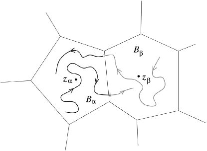
If we were to generate an infinitely long trajectory of the system, ${\boldsymbol{z}}(t)$ with $t>0$, this trajectory would keep going in and out of the cells $B_{\alpha}$ by crossing the edges between these cells. Out of this trajectory we could therefore generate an ensemble of exit-entry points, i.e. those points on the edges of the cells at which the trajectory goes from a cell $B_{\alpha}$ into a neighboring cell $B_{\beta}$. By the Markovian assumption, these points are all we need to generate an exact sample of trajectories inside each of the cells $B_{\alpha}$ simply by starting trajectories at the points leading into that cell and running these trajectories forward in time until they exit the cell. The procedure in Refs. warmflashJCP07, ; dicksonJCP09, is a way to generate these pieces of trajectories inside the cells without having to compute the entry points beforehand from a long unbiased trajectory but rather by generating them on-the-fly. To understand how this is done, imagine that we associate an independent copy, or replica, of the system to each cell $B_{\alpha}$. Let us denote the instantaneous position of these replicas by ${\boldsymbol{z}}_{\alpha}(t)\in B_{\alpha}$, $\alpha=1,\ldots,\Lambda$. Even if we start ${\boldsymbol{z}}_{\alpha}(t)$ inside $B_{\alpha}$, sooner or later this trajectory will try to exit $B_{\alpha}$ and go to another cell. When this happens, we store the exit point on the boundary, put the trajectory on hold and wait until a trajectory in one of the neighboring cells makes an attempt to exit this cell by crossing the boundary with $B_{\alpha}$. We then take this crossing point and use it to reinitialize the trajectory in $B_{\alpha}$. This is illustrated in Fig. 1. At the beginning of the simulation we do not have enough re-entry points, so many of the replicas may be on hold. But as the simulation goes on, we can build databanks of re-entry points from any $B_{\beta}$ into any $B_{\alpha}$ (assuming that these two cells have a common boundary – otherwise the databank is trivially empty), which contain the last $X$ points by which the trajectory tried to escape from cell $B_{\beta}$ and enter cell $B_{\alpha}$. This way, each time a trajectory tries to exit a cell $B_{\alpha}$, we can immediately pick a re-entry point into that cell from the appropriate databank and continue the trajectory from that point without having to put it on hold.

The only remaining issue we need to take care of in order to make complete the procedure outlined above is how to pick the re-entry point into $B_{\alpha}$ among the databanks on the various edges leading into $B_{\alpha}$. By construction, the re-entry points in the databanks on each edge are unbiased samples of re-entry points conditional on the trajectory entering by that edge. But there are several edges by which the trajectory can enter a given cell, and to introduce no bias we need to pick the edges with the proper probability of re-entrance by that edge. To see how this can be done, imagine that, as we run the simulation in each cell $B_{\alpha}$, we compute an estimate of the effective rate of exit out that cell and into $B_{\beta}$ via

$$\nu_{\alpha,\beta}=\frac{N_{\alpha,\beta}}{T_{\alpha}}$$ (2)

where $N_{\alpha,\beta}$ is the total number of times the trajectory hit the boundary between $B_{\alpha}$ and $B_{\beta}$ (which is also the number of times the trajectory in cell $B_{\alpha}$ had to be re-injected into that cell from a re-entry point) and $T_{\alpha}$ is the total simulation time in cell $B_{\alpha}$ (i.e. the total time the trajectory in cell $B_{\alpha}$ was running). If we then denote by $\pi_{\alpha}$ the probability to find the unbiased trajectory inside cell $B_{\alpha}$ at statistical steady state, i.e.

$$\pi_{\alpha}=\int_{B_{\alpha}}\varrho({\boldsymbol{z}})d{\boldsymbol{z}},$$ (3)

we see that $\pi_{\alpha}$ and $\nu_{\alpha,\beta}$ are related as

$$\sum_{\begin{subarray}{c}\beta=1\\ \beta\not=\alpha\end{subarray}}^{\Lambda}\pi_{\beta}\nu_{\beta,\alpha}=\sum_{\begin{subarray}{c}\beta=1\\ \beta\not=\alpha\end{subarray}}^{\Lambda}\pi_{\alpha}\nu_{\alpha,\beta},\qquad\sum_{\alpha=1}^{\Lambda}\pi_{\alpha}=1.$$ (4)

The first equation in (4) simply expresses that, at statistical steady state, the total probability flux into $B_{\alpha}$ (which is the term at the left hand-side of the first equation in (4)) must be equal to the total flux out of $B_{\alpha}$ (which is the term at the right hand-side of the first equation in (4)). The second equation in (4) is simply a normalization condition for the probability which follows from $\sum_{\alpha}\pi_{\alpha}=\sum_{\alpha}\int_{B_{\alpha}}\varrho({\boldsymbol{z}})d{\boldsymbol{z}}=\int_{\Omega}\varrho({\boldsymbol{z}})d{\boldsymbol{z}}=1$. We stress that (4) does not require detailed balance (i.e. $\pi_{\beta}\nu_{\beta,\alpha}\not=\pi_{\alpha}\nu_{\alpha,\beta}$, possibly) and so it holds even for nonequilibrium processes provided only that they are at statistical steady state. Having calculated $\nu_{\alpha,\beta}$ from (2) and $\pi_{\alpha}$ from (4), we then have an estimate for the probability flux from $B_{\beta}$ into $B_{\alpha}$: $\pi_{\beta}\nu_{\beta,\alpha}$. Consistently, the probability that the trajectory enters cell $B_{\alpha}$ by coming from $B_{\beta}$ is simply:

$$\mathbb{P}_{\partial B_{\beta}\cap\partial B_{\alpha}}=\frac{\pi_{\beta}\nu_{\beta,\alpha}}{\sum_{\beta^{\prime}\neq\alpha}\pi_{\beta^{\prime}}\nu_{\beta^{\prime},\alpha}},\quad(\beta\neq\alpha),$$ (5)

if $B_{\alpha}$ and $B_{\beta}$ have a common edge and $\mathbb{P}_{\partial B_{\beta}\cap\partial B_{\alpha}}=0$ otherwise. This expression gives us the desired probability to pick the edge $\partial B_{\beta}\cap\partial B_{\alpha}$ for re-entry into $B_{\alpha}$.

Summarizing, the algorithm to perform simulations restricted inside the cells for systems at nonequilibrium steady state is as follows:

• Denoting by ${\boldsymbol{z}}_{\alpha}(t)\in B_{\alpha}$ the current state of the replica in cell $B_{\alpha}$, let ${\boldsymbol{z}}_{\alpha}^{\star}$ be the state of the system produced from ${\boldsymbol{z}}_{\alpha}(t)$ after one timestep $\mathit{\Delta}t$ by a standard (i.e. unrestricted) integrator for the system (e.g. velocity-Verlet if the system is a molecular dynamics (MD) system). If ${\boldsymbol{z}}^{\star}_{\alpha}\in B_{\alpha}$, set

  $${\boldsymbol{z}}_{\alpha}(t+\mathit{\Delta}t)={\boldsymbol{z}}^{\star}_{\alpha}.$$ (6)

  Otherwise, if ${\boldsymbol{z}}^{\star}_{\alpha}\in B_{\beta}$ with $\beta\neq\alpha$:

  • Store the point ${\boldsymbol{z}}_{\alpha}^{\star}$ in a databank of entry points from $B_{\alpha}$ into $B_{\beta}$. In other words, assuming that the databank contains already $m$ points ${\boldsymbol{z}}_{\alpha,\beta}^{k}$ with $k=1,2,\ldots,m$, set ${\boldsymbol{z}}_{\alpha,\beta}^{m+1}={\boldsymbol{z}}_{\alpha}^{\star}$.

  • Update $\nu_{\alpha,\beta}$ via (2), $\pi_{\alpha}$ via (4) and $\mathbb{P}_{\partial B_{\beta}\cap\partial B_{\alpha}}$ via (5).

  • Select an edge $\partial B_{\beta^{\prime}}\cap\partial B_{\alpha}$ of $B_{\alpha}$ with probability proportional to $\mathbb{P}_{\partial B_{\beta^{\prime}}\cap\partial B_{\alpha}}$.

  • Pick a point ${\boldsymbol{z}}_{\beta^{\prime},\alpha}^{k}$ with uniform probability from the databank of re-entry points on edge $\partial B_{\beta^{\prime}}\cap\partial B_{\alpha}$, and set

    $${\boldsymbol{z}}_{\alpha}(t+\mathit{\Delta}t)={\boldsymbol{z}}_{\beta^{\prime},\alpha}^{k}$$ (7)

• Go to step (1) and iterate to collect statistics.

In essence, the algorithm above is the same as the one proposed in Ref. warmflashJCP07, ; dicksonJCP09, , though the two differ in the details. For instance, we use a single set of cells instead of two (in Refs. warmflashJCP07, ; dicksonJCP09, two staggered sets were used to ensure stability, but we observed no such stability problems with the procedure above). Besides a set of trajectories, one of the output of the procedure is to give the probability $\pi_{\alpha}$ to find the system in cell $B_{\alpha}$ at statistical steady state (see (3)). Indeed the computation of $\pi_{\alpha}$ was the main objective in Refs. warmflashJCP07, ; dicksonJCP09, . Below we will show how to extract more from the procedure, in particular reaction rate information, by appropriate modifications. Before getting there, however, let us make a few remarks about the algorithm above. In step (iv) we have assumed that the list of entry points from $B_{\beta^{\prime}}$ into $B_{\alpha}$ is not empty and, as already mentioned above, this may not be true at the beginning of the simulation (there might have been no collision with that edge up to that time). In that case we have to put the simulations in some of cells on hold at the beginning until we get proper re-entry points and start building databanks on the edges. Note that, at any given time, these databanks could each contain the last re-entry point only, though in that case we may run out of points again and have to put replicas on hold. Thus it is safer to always keep as many points in the databanks as memory allows. However, the databanks do not have to be enlarged indefinitely – at worst we trade memory for CPUs since, the smaller the databanks, the higher the probability that one replica will have to be put on hold for some time. Also note that the quantities used to evaluate the probability in Eq. (5) have to be computed on-the-fly, and need information from all the cells. This, again, may lead to problems at the beginning of the simulations, when the statistics for $N_{\alpha,\beta}$ is not accurate enough. To overcome this problem we set $\pi_{\alpha}=cst$ $\forall\alpha=1,\ldots,N$ at the beginning when statistics is insufficient to solve Eq. (4). Using more educated guesses is possible too. Also, it is worth noting that $\nu_{\alpha,\beta}$ and $\pi_{\alpha}$ can be monitored on-the-fly to assess their convergence as a function of the length of the simulation, and the actual simulations of the replicas in each cell can be performed in parallel; only the re-entry events require communication. Finally, we should stress that the procedure above relies on the ability to count the successive points at which a trajectory crosses the edges of the cells. This may lead to difficulties if the dynamics is governed by a stochastic differential equation, in which case these crossing points may form a fractal set. It leads to no difficulty, however, if some components of the trajectory are smooth and the cells are defined accordingly. We will come back to this issue later in the illustrative example section.

Rate calculation.

Let us now come to the question of how to compute the reaction rate between a reactant and product state, which we identify as two disjoint sets in the system’s state-space denoted as $A\subset\Omega$ and $B\subset\Omega$ respectively. As mentioned earlier, this calculation will be done by twisting the dynamics in some appropriate way that is dictated by the results of TPT. We begin by introducing the relevant objects that we will consider. If we assume again that we have at our disposal an infinitely long trajectory, ${\boldsymbol{z}}(t)$ with $t>0$, this trajectory will go back and forth between $A$ and $B$ as time goes on, and we can split this trajectory into two pieces, depending on whether it visited last $A$ or $B$. This construction is illustrated in Fig. 2, where the trajectory is shown in red if it visited $A$ last and in black if it visited $B$ last: if the trajectory visited $A$ last at time $t$, we will say that it is assigned to $A$ at time $t$, if it visited $B$ last at time $t$, we will say that it is assigned to $B$ at time $t$.

Figure 2: Schematic representation of a piece of ergodic trajectory visiting the two sets $A$ and $B$. The pieces of this trajectory for which the last visited set was $A$ are depicted in red, and those for which the last visited set was $B$ are depicted in black.

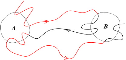
Based on this assignment, we can introduce the following quantities. If $N^{T}_{A,B}$ denotes the total number of times the trajectory went from being assigned to $A$ to being assigned to $B$ during the time interval $[0,T]$ (i.e. the number of times it switched from red to black in Fig. 2), we set

$$\nu_{R}=\lim_{T\to\infty}\frac{N^{T}_{A,B}}{T}.$$ (8)

This quantity gives the average frequency at which the trajectory goes from $A$ to $B$ which, because the system is at steady state, is also the same as the average frequency at which the trajectory goes from $B$ to $A$ since $N^{T}_{A,B}=N^{T}_{B,A}$ asymptotically. The rate in (8) is referred to as the rate of the reactive trajectories in TPT, hence the subscript $R$. The rate of reactive trajectories $\nu_{R}$ should not be confused with the two reaction rates from $A$ to $B$ and $B$ to $A$ defined respectively as

$$k_{A,B}=\lim_{T\to\infty}\frac{N^{T}_{A,B}}{T_{A}},\quad k_{B,A}=\lim_{T\to\infty}\frac{N^{T}_{A,B}}{T_{B}},$$ (9)

where $T_{A}$ and $T_{B}$ are, respectively, the total times during which the trajectory was assigned to $A$ or $B$ in the interval $[0,T]$ (i.e. the total times the trajectory is red or black in Fig. 2). If $A$ and $B$ are metastable (i.e. if the trajectory commits to each of these sets and looses memory of its past before going back to the other set), $k_{A,B}$ and $k_{B,A}$ are the rates that enter the phenomenological mass-action law describing how the populations in $A$ and $B$ evolve in time. Notice that $\nu_{R}$ is related to $k_{A,B}$ and $k_{B,A}$ as

$$k_{A,B}=\frac{\nu_{R}}{\rho_{A}},\qquad k_{B,A}=\frac{\nu_{R}}{\rho_{B}},$$ (10)

where $\rho_{A}$ is the fraction of time the trajectory is assigned to $A$ and $\rho_{B}$ the fraction of time it is assigned to $B$:

$$\rho_{A}=\lim_{T\to\infty}\frac{T_{A}}{T},\qquad\rho_{B}=\lim_{T\to\infty}\frac{T_{B}}{T}.$$ (11)

By definition $\rho_{A}\leq 1$, $\rho_{B}\leq 1$ and $\rho_{A}+\rho_{B}=1$. The quantities $\nu_{R}$, $k_{A,B}$, $k_{B,A}$, $\rho_{A}$ and $\rho_{B}$ are the ones we will show how to compute exactly. To see how this can be done, it is useful to give first the TPT expressions for these quantities. These expressions involve the backward committor function, $q_{-}({\boldsymbol{z}})$, which gives the probability that a trajectory observed at point ${\boldsymbol{z}}$ is coming from $A$ last rather than from $B$ (i.e. that it is assigned to $A$ rather than $B$ using the jargon introduced above). By definition $q_{-}({\boldsymbol{z}})=1$ if ${\boldsymbol{z}}\in A$, $q_{-}({\boldsymbol{z}})=0$ if ${\boldsymbol{z}}\in B$, and $0\leq q_{-}({\boldsymbol{z}})\leq 1$ otherwise. The backward committor function is useful because by the Markovian assumption it follows that, at statistical steady state, the probability density to observe a trajectory at point ${\boldsymbol{z}}\in\Omega$ at any given time $t$ and that this trajectory is assigned to $A$ at that time is simply $\varrho_{A}({\boldsymbol{z}})=\varrho({\boldsymbol{z}})\,q_{-}({\boldsymbol{z}})$. Similarly the probability density to observe a trajectory at point ${\boldsymbol{z}}\in\Omega$ at time $t$ and that this trajectory is assigned to $B$ at that time is $\varrho_{B}({\boldsymbol{z}})=1-\varrho_{A}({\boldsymbol{z}})=\varrho({\boldsymbol{z}})\,(1-q_{-}({\boldsymbol{z}}))$. Since $\rho_{A}=\int_{\Omega}\varrho_{A}({\boldsymbol{z}})d{\boldsymbol{z}}$ and $\rho_{B}=\int_{\Omega}\varrho_{B}({\boldsymbol{z}})d{\boldsymbol{z}}$ by definition, this implies that

$$\rho_{A}=\int_{\Omega}\varrho({\boldsymbol{z}})\,q_{-}({\boldsymbol{z}})\,d{\boldsymbol{z}}\leq 1,\qquad\rho_{B}=1-\rho_{A}.$$ (12)

Similarly, it is easy to see that $\nu_{R}$ is the total probability flux associated with $\varrho_{A}({\boldsymbol{z}})=\varrho({\boldsymbol{z}})\,q_{-}({\boldsymbol{z}})$ going through any dividing surface between $A$ and $B$ (like e.g. the boundary of $B$). The explicit form of this flux depends on the specifics of the dynamics and it is given in Ref. tpt_erice, : let us omit to repeat this formula here since it will not be important in what follows.

Figure 3: Schematic illustration of a piece of trajectory crossing the cells $B_{\alpha}$ with $\alpha=1,\ldots,5$, where cell $B_{1}$ is identified with the reactant state $A$ and cell $B_{5}$ with the product state $B$. The circles represent the entry points which would be used to perform sampling restricted in the cells. If only the red points are used as re-entry points, then the restricted sampling selects the pieces of this trajectory when it is assigned to $A$ (these pieces are depicted in red).

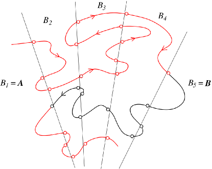
In practice, we do not know explicitly $q_{-}({\boldsymbol{z}})$ (nor even $\varrho({\boldsymbol{z}})$ in most nonequilibrium systems) but we can still make use of the observations above to modify the sampling procedure explained before. Suppose that we define the reactant state $A$ as being the union of a group of cells $B_{\alpha}$ and the product state $B$ as the union of another group. Clearly, what we would then like to do is modify the sampling procedure in such a way that only the re-entry points associated with the trajectory when it is assigned to $A$ are put in the databanks (see the illustration in Fig. 3) and keep track of the associated probability fluxes through the boundary of the cells. Indeed, using these re-entry points and these fluxes only, we would then simulate in the cells pieces of trajectories that are statistically indistinguishable from the unbiased trajectory when it is assigned to $A$. We could then compute the total probability in the cells to get an estimate of $\rho_{A}$ (and hence $\rho_{B}=1-\rho_{A}$) as well as the total flux into $B$ to get $\nu_{R}$. We claim that there is a simple procedure to do these operations in practice. The key observation is that trajectories assigned to $A$ can be propagated like regular trajectories while they are outside of $A$ and $B$ – the only constraint imposed on them is via a boundary condition in their past: they need to have come from $A$ rather than $B$ last. But we know what this boundary condition entails, at least in a statistical sense: indeed the probability density $\varrho_{A}({\boldsymbol{z}})$ that a trajectory be at ${\boldsymbol{z}}$ and be assigned to $A$ is equal to the statistical steady state probability density $\varrho({\boldsymbol{z}})$ for ${\boldsymbol{z}}\in A$ while it is equal to 0 for ${\boldsymbol{z}}\in B$. We also know that the probability flux out of $A$ is the statistical steady state one and the probability flux out of $B$ is identically zero.

We can easily impose these boundary conditions in practice by modifying our sampling procedure as follows. Suppose that we have performed a sampling as before and computed the steady state (unbiased) $\pi_{\alpha}$ and $\nu_{\alpha,\beta}$. We can then run another independent sampling where we only consider the cells outside of $A$ and $B$. In these cells, we run trajectories as before (though, as we will see, using re-entry points that are different from the ones calculated before), store their exit points from the cells to build databanks of re-entry points in other cells, and compute

$$\nu^{A}_{\alpha,\beta}=\frac{N^{A}_{\alpha,\beta}}{T^{A}_{\alpha}}$$ (13)

where $N^{A}_{\alpha,\beta}$ is the total number of times the trajectories hit the boundary between $B_{\alpha}$ and $B_{\beta}$ and $T^{A}_{\alpha}$ is the total simulation time in cell $B_{\alpha}$. Note that $\nu^{A}_{\alpha,\beta}$ is only defined by (13) if $\alpha$ is the index of a cell $B_{\alpha}$ not inside $A$ and $B$ (the index $\beta$, on the other hand, runs over all the cells, including those forming $A$ and $B$). Consistent with the bias we need to impose to focus on trajectories assigned to $A$, we supplement this by $\nu_{\alpha,\beta}^{A}=\nu_{\alpha,\beta}$ if $\alpha$ is the index of a cell $B_{\alpha}$ used to define $A$ (since the effective rate of exit out of $A$ must be the unbiased statistical steady one) and by $\nu_{\alpha,\beta}^{A}=0$ if $\alpha$ is the index of a cell $B_{\alpha}$ used to define $B$ (since the effective rate of exit out of $B$ must be zero). We also set $\pi^{A}_{\alpha}=\pi_{\alpha}$ if $\alpha$ is the index of a cell $B_{\alpha}$ used to define $A$, $\pi^{A}_{\alpha}=0$ if $\alpha$ is the index of a cell $B_{\alpha}$ used to define $B$, and in all the other cells we compute $\pi^{A}_{\alpha}$ via

$$\sum_{\begin{subarray}{c}\beta=1\\ \beta\not=\alpha\end{subarray}}^{\Lambda}\pi^{A}_{\beta}\nu^{A}_{\beta,\alpha}=\sum_{\begin{subarray}{c}\beta=1\\ \beta\not=\alpha\end{subarray}}^{\Lambda}\pi^{A}_{\alpha}\nu^{A}_{\alpha,\beta}$$ (14)

where the index $\alpha$ runs over all the cells outside of $A$ and $B$ and we use as boundary conditions the values for $\nu_{\beta,\alpha}^{A}$ and $\pi^{A}_{\beta}$ set before when the index $\beta$ is that of a cell used to define $A$ or $B$. Finally, we compute the probability of re-entry on the edges of a cell $B_{\alpha}$ not inside $A$ and $B$ as

$$\mathbb{P}^{A}_{\partial B_{\beta}\cap\partial B_{\alpha}}=\frac{\pi^{A}_{\beta}\nu^{A}_{\beta,\alpha}}{\sum_{\beta^{\prime}\neq\alpha}\pi^{A}_{\beta^{\prime}}\nu^{A}_{\beta^{\prime},\alpha}},\quad(\beta\neq\alpha).$$ (15)

This procedure automatically guarantees that we focus on the trajectories assigned to $A$ and makes all the quantities above – the set of trajectories, the databanks, $\nu^{A}_{\alpha,\beta}$ and $\pi^{A}_{\alpha}$ – different from their unbiased statistical steady state counterparts. By construction we then have $\pi^{A}_{\alpha}=\int_{B_{\alpha}}\varrho_{A}({\boldsymbol{z}})d{\boldsymbol{z}}$ which, from (12), means that

$$\rho_{A}=\sum_{\alpha=1}^{\Lambda}\pi_{\alpha}^{A}\leq 1,\qquad\rho_{B}=1-\rho_{A}.$$ (16)

Similarly we can compute $\nu_{R}$ from the total flux into $B$:

$$\nu_{R}=\sum_{\begin{subarray}{c}\text{$\alpha$ such that}\\ \text{$B_{\alpha}$ not in $B$}\end{subarray}}\ \ \sum_{\begin{subarray}{c}\text{$\beta$ such that}\\ \text{$B_{\beta}$ in $B$}\end{subarray}}\pi^{A}_{\alpha}\nu_{\alpha,\beta}^{A}.$$ (17)

Finally, we can get $k_{A,B}$ and $k_{B,A}$ from (10) and be done.

Comparison with TIS, FFS, and Markovian milestoning with Voronoi tessellations.

Before illustrating our procedure to compute the reaction rate on a simple example, let us compare it to existing methods. First, let us point out that it is very similar in spirit to both TIS tis2 ; pptis ; tis3 and FFSffs ; valerianiFFS . Like TIS and FFS, our method is based on selecting only those trajectories which come from the reactant state $A$. The difference is in the way this selection is achieved. In particular, unlike in TIS and FFS, we do not require that the interfaces be ordered monotonously, i.e. we do not need that a trajectory coming from $A$ crosses all the preceding interfaces before reaching the next one. This offers more flexibility in the way the interfaces can be chosen. Here we did so using the edges of cells in a Voronoi tessellation because it is convenient, but the formalism above is clearly independent of that choice and can be applied to any type of interfaces.

Regarding the relation with the Markovian milestoning procedure with Voronoi tessellation miles6 , the main advantage of the method proposed in this note to compute the rate is that it is exact and hence avoids completely the assumptions underlying milestoning miles5 . On the other hand, the new procedure is also more costly since it requires not only to build databanks of re-entry points but also to do the sampling twice – once to get the unbiased statistical steady states quantities, and once more to get the reaction rate by twisting the dynamics. For systems at equilibrium, one may therefore prefer to use the Markovian milestoning procedure with Voronoi tessellation miles6 which is cheaper. For nonequilibrium systems, this procedure is inapplicable (since it relies on the time-reversibility of the dynamics), but as a compromise, one could use the nonequilibrium sampling strategy for the unbiased system to compute the relevant quantities in Markovian milestoning and thereby avoid to make the second twisted sampling to compute the rate. Indeed, the formalism developed in Ref. miles6, to approximate the dynamics by a continuous-time Markov chain does not rely on the dynamics being at equilibrium. For completeness let us briefly recall the main objects in Markovian milestoning and indicate how to compute them in the present context. If, following Ref. miles6, , we define the milestones as the common boundaries between any two adjacent Voronoi cells and denote these milestones by $S_{i}$ with $i=1,2,\dots,N$, the key quantity to approximate the transitions between the milestones by a continuous-time Markov chain is the rate matrix whose off-diagonal elements can be estimated as

$$q_{ij}=\begin{cases}N_{ij}/R_{i}\quad&\text{if $R_{i}\neq 0$}\\ \quad 0\quad&\text{if $R_{i}=0$}.\end{cases}$$ (18)

where

$$N_{ij}=\sum_{\alpha=1}^{\Lambda}\pi_{\alpha}\frac{N_{ij}^{\alpha}}{T_{\alpha}},\qquad R_{i}=\sum_{\alpha=1}^{\Lambda}\pi_{\alpha}\frac{R_{i}^{\alpha}}{T_{\alpha}}.$$ (19)

Here $T_{\alpha}$ is the total simulation time in cell $B_{\alpha}$ (as before), whereas $N_{ij}^{\alpha}$ is the total number of times the trajectory went from milestone $S_{i}$ to milestone $S_{j}$ and $R_{i}^{\alpha}$ is the total amount of time the trajectory is assigned to milestone $S_{i}$ in cell $B_{\alpha}$, i.e. the total amount of time this trajectory is such that $S_{i}$ was the edge of cell $B_{\alpha}$ it hit last. We refer the reader to Ref. miles6, for more details.

Figure 4: Contourplot of the Mueller potential with the 36 points (shown as grey dots) generating the Voronoi tessellation shown as grey lines. The reactant $A$ and product $B$ states are identified with cell $B_{1}$ and $B_{36}$, respectively.

Illustrative example.

We end this note by illustrating our sampling procedure on the example of a system evolving by Langevin dynamics on a two-dimensional potential, i.e. ${\boldsymbol{z}}(t)=({\boldsymbol{x}}(t),{\boldsymbol{v}}(t))$, ${\boldsymbol{x}},{\boldsymbol{v}}\in\mathbb{R}^{2}$ and

$$\begin{cases}\dot{\boldsymbol{x}}(t)={\boldsymbol{v}}(t),\\ \dot{\boldsymbol{v}}(t)=-\nabla V({\boldsymbol{x}}(t))-\gamma{\boldsymbol{v}}(t)+\sqrt{2\beta^{-1}\gamma}\,{\boldsymbol{\eta}}(t).\end{cases}$$ (20)

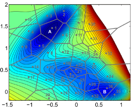
Here $V({\boldsymbol{x}})$ is the Mueller potential mueller whose contourplot is shown in Fig. 4, $\beta=1/(k_{B}T)$ is the inverse temperature and ${\boldsymbol{\eta}}(t)$ is a Gaussian white-noise with mean zero and covariance $\langle\eta_{i}(t)\eta_{j}(t^{\prime})\rangle=\delta_{ij}\delta(t-t^{\prime})$. $\gamma$ is the friction coefficient and, for simplicity, we have set the mass tensor to the identity. Below we took $\gamma=100$ and $\beta^{-1}=20$ (which is about $20\%$ the value of the energy barrier between the minimum at the top left corner of the Mueller potential and the saddle point at (-0.8,0.6)). This example is obviously very simple and serves no other purpose than being a benchmark: the application of our sampling procedure to more interesting examples will be reported elsewhere. To avoid confusions, before presenting our results for (20) let us note that this system is an equilibrium one, with equilibrium density $\varrho({\boldsymbol{x}},{\boldsymbol{v}})=Z^{-1}\exp(-\beta H({\boldsymbol{x}},{\boldsymbol{v}}))$ where $H({\boldsymbol{x}},{\boldsymbol{v}})=\frac{1}{2}|{\boldsymbol{v}}|^{2}+V({\boldsymbol{x}})$ is the Hamiltonian and $Z=\int_{\mathbb{R}^{2}\times\mathbb{R}^{2}}\exp(-\beta H({\boldsymbol{x}},{\boldsymbol{v}}))d{\boldsymbol{x}}d{\boldsymbol{v}}$ the partition function. We are, however, primarily interested in computing the reaction rates between the reactant state $A$ and the product state $B$ shown in Fig. 4, which we will achieve by twisting the dynamics as explained before to focus on trajectories assigned to $A$. In so doing, we automatically put the system out of equilibrium since $A$ becomes a source and $B$ a sink (and $\varrho_{A}({\boldsymbol{x}},{\boldsymbol{v}})\not=\varrho({\boldsymbol{x}},{\boldsymbol{v}})$). This is why we need the nonequilibrium formalism developed above to compute reaction rates even in the case of an equilibrium system such as (20).

Shown in Fig. 4 are the 36 cells that we used in our calculations. These cells were defined as

$$B_{\alpha}=\{({\boldsymbol{x}},{\boldsymbol{v}})\in\mathbb{R}^{2}\times\mathbb{R}^{2}\;:\;|{\boldsymbol{x}}- {\boldsymbol{x}}_{\alpha}|<|{\boldsymbol{x}}-{\boldsymbol{x}}_{\beta}|$$ (21)

$$\text{for all}\;\beta\neq\alpha\},$$

where $|\cdot|$ denotes the Euclidean norm and ${\boldsymbol{x}}_{\alpha}$ with $\alpha=1,\ldots,36$ are points chosen randomly in the region where the energy is below a certain threshold value. We identified the reactant and product states with two single cells in the neighborhood of the two deep minima in the potential landscape: $A=B_{1}$ and $B=B_{36}$ (see Fig 4). Note that we intentionally took many cells and disposed them in a way that may not be optimal for the reaction to check that our procedure is robust against such choices. Note also that by defining the cells primarily in position space as we do in (21) we guarantee that we can count successive crossing of their boundaries. This would not be the case if the boundaries of the cells were bent in velocity space, because of the noise term in (20) that acts on the velocities.

Both steps of the sampling procedure (the one to compute the unbiased equilibrium quantities and the other with the twisted dynamics) were performed as described above by running simulations for $10^{8}$ steps in each cell using the second order integrator of Ref. langevin, with a timestep $\mathit{\Delta t}=10^{-4}$. In the first step of the procedure we took $\pi_{\alpha}$ equal in each cell as initial condition; in the second step, we took $\pi_{\alpha}^{A}=\pi_{\alpha}$ as initial condition. We compared the results of our procedure with those obtained by generating a long ($10^{10}$ steps) unbiased trajectory by brute force simulation and computing $\nu_{R}$, $k_{A,B}$ and $k_{B,A}$ from finite $T$ approximations of the limits in (8) and (9).

	$\nu_{R}$	$k_{A,B}$	$k_{B,A}$
Twisted dynamics	$5.9\,10^{-3}$	$7.4\,10^{-3}$	$3.1\,10^{-3}$
Direct simulation	$5.8\,10^{-3}$	$7.1\,10^{-3}$	$3.2\,10^{-3}$

Table 1: Rate of reactive trajectories and reaction rates between the sets $A$ and $B$ in the Mueller potential (see Fig. 4) obtained by the procedure presented here and by direct calculation using a long unbiased trajectory.

Figure 5: Probability $\pi_{\alpha}$ to be in the cells (semi-log scale) obtained via sampling restricted in the Voronoi cells (black dots) and by a brute force unbiased trajectory (triangles). The agreement is excellent. Also shown as circles are the steady state nonequilibrium probabilities $\pi^{A}_{\alpha}$ of the twisted dynamics. Note that by construction $\pi^{A}_{36}=0$ (since $B_{36}=B$) and we did not plot this point.

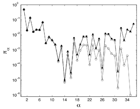
The main outputs of our procedure are the rate of reactive trajectories $\nu_{R}$ and the reaction rates $k_{A,B}$ and $k_{B,A}$ which are reported in Table 1. These are within statistical errors of the corresponding quantities estimated by brute force simulation. Our procedure also produces the equilibrium probabilities $\pi_{\alpha}$: as shown in Fig. 5 these are within statistical errors of the corresponding values obtained by the brute force simulation. Also shown in Fig. 5 are the probabilities $\pi_{\alpha}^{A}$ computed by twisting the dynamics. As expected, the closer to $B$, the smaller $\pi_{\alpha}^{A}$ is compared to $\pi_{\alpha}$.

References

- (1) A. Warmflash, P. Bhimalapuram, and A. R. Dinner, J. Chem. Phys. 127, 154112 (2007).
- (2) A. Dickson, A. Warmflash, and A. R. Dinner, J. Chem. Phys. 130, 074104 (2009).
- (3) W. E and E. Vanden-Eijnden, J. Stat. Phys. 123, 503 (2006).
- (4) E. Vanden-Eijnden, Transition path theory, in Computer Simulations in Condensed Matter: From Materials to Chemical Biology - Vol. 1, edited by M. Ferrario, G. Ciccotti, and K. Binder, pages 439–478, Berlin, 2006, Springer.
- (5) P. Metzner, C. Schütte, and E. Vanden-Eijnden, J. Chem. Phys. 125, 084110 (2006).
- (6) E. Vanden-Eijnden and M. Venturoli, J. Chem. Phys. (2009), Accepted for publication.
- (7) A. K. Faradjian and R. Elber, J. Chem. Phys. 120, 10880 (2004).
- (8) A. M. A. West, R. Elber, and D. Shalloway, J. Chem. Phys. 126, 145104 (2007).
- (9) R. Elber, Biophys. J. 92, L85 (2007).
- (10) E. Vanden-Eijnden, M. Venturoli, G. Ciccotti, and R. Elber, J. Chem. Phys. 129, 174102 (2008).
- (11) D. Moroni, T. S. van Erp, and P. G. Bolhuis, Physica A 340, 395 (2004).
- (12) D. Moroni, P. G. Bolhuis, and T. S. van Erp, J. Chem. Phys. 120, 4055 (2004).
- (13) T. S. van Erp and P. G. Bolhuis, J. Comput. Phys. 205, 157 (2005).
- (14) R. J. Allen, D. Frenkel, and P. R. ten Wolde, J. Chem. Phys. 124, 024102 (2006).
- (15) C. Valeriani, R. J. Allen, M. J. Morelli, D. Frenkel, and P. R. ten Wolde, J. Chem. Phys. 127, 114109 (2007).
- (16) E. Vanden-Eijnden and M. Venturoli, J. Chem. Phys. (2009), Accepted for publication.
- (17) K. Mueller, Angew. Chem. 19, 1 (1980).
- (18) E. Vanden-Eijnden and G. Ciccotti, Chem. Phys. Lett. 429, 310 (2006).