Determination of Low Energy Constants and testing Chiral Perturbation Theory at Next to Next to Leading Order

Abstract:

We present the results of a search for relations between observables that are independent of the Chiral Pertubation Theory (ChPT) Next-to-Next-to-Leading Order (NNLO) Low-Energy Constants (LECs). We have found some relations between observables in $\pi\pi$, $\pi K$ scattering and $K_{l4}$ decay which have been evaluated numerically using the old fit (fit 10 in [1]) of the NLO LECs.

1 Introduction

As pointed out in many talks in this conference one of the major problems of ChPT is the determination of the LECs. This is an issue that has to be solved if we want a complete predictive theory and to check its convergence. Furthermore, since the LECs encode the dynamics of the underlying theory QCD, they can in principle provide us with more information on it as well.

On the other hand, chiral symmetry imposes no constraints on the values of the coupling constants, thus we need to perform a fit for their determination. This is a rather difficult task for different reasons.

First of all, going to higher order in the chiral expansion the number of independent operators allowed by the symmetries in the Lagrangians, and therefore the number of coupling constants to estimate, increases. E.g., in $SU(3)$ ChPT up to NNLO, the following LECs appear: $2$ in $\mathcal{L}_{2}$ $(F_{0},B_{0})$, $10+2$ in $\mathcal{L}_{4}$ $(L_{i}s,H_{i}s)$ and $90+4$ in $\mathcal{L}_{6}$ $(C_{i})$s.

Moreover these constants are strongly correlated. As a matter of fact since at order $p^{6}$ typically many $L_{i}$s contribute to particular processes, their determination entangles different processes. As a result, an estimate of an order $p^{6}$ LEC used in one process where an $L_{i}$ is determined sneaks in the determination of the other $L_{i}$s and possibly of the $C_{i}$s in the other processes. The solution, a full comprehensive analysis of all processes at the same time, is a major undertaking which has not been done [2].

Finally, so far we don’t have enough data to perform a complete fit of all the constants, even if in this regard other kinds of results, such as dispersive and lattice calculations, are helpful.

The solution which has been mainly used so far is to perform the fit of the $L_{i}$s relying on estimates of the values of the $C_{i}$s by simple resonance saturation, see the discussion in [1, 3], but now we have at our disposal a lot of processes calculated up to NNLO (see [2] for a review) and new measurements of the obsevables involved, thus it is time to collect all this knowledge and perform a new global fit.

As said above, one of the main problems to overcome when performing the fit is the large number of unknown constants appearing at NNLO. For this purpose we have looked for relations between observables that do not involve the $C_{i}$.

If $O$ is an observable, then ChPT allows us to write it is as a sum of terms of increasing importance in the chiral expansion:

$$O = O^{(2)}+O^{(4)}+O^{(6)}\,.$$ (1)

The $p^{6}$ part can be split as

$$O^{(6)} = O_{C_{i}{\rm(tree\,level)}}+O_{L_{i}\rm{(one\,loop)}}+O_{F_{0}\rm{(two\,loops)}}.$$ (2)

We found relations between observables such that the first contribution, the only one where the $C_{i}$ dependence shows up, cancels out. Using these relations we can stop worrying about the $C_{i}$s and perform the fit of the $L_{i}$s at NNLO. Moreover we can check how large the loop contributions are and thus test ChPT convergence.

So far we considered the following processes and quantities: $\pi\pi$ and $\pi K$ scattering, $K_{l4}$ $(K\rightarrow\pi\pi e\nu)$, scalar form factors $(F_{S}^{\pi/K}(t))$, meson masses, meson decay constants ($F_{\pi/K}$), vector form factors $(F^{\pi/K}_{V})$ and $\eta\rightarrow\pi\pi\pi$. We found many relations, but not all of them are equally useful for the fit purpose: some of them involve not yet well known observables and some others are long and complicated expressions. Hence in the following we only quote the most relevant ones. All results presented are preliminary. We discuss now the relations and then a first numerical check of some of them.

2 Relations between Observables

2.1 $\pi\pi$ scattering

The $\pi\pi$ scattering amplitude can be written as a function $A(s,t,u)$ which is symmetric in the last two arguments:

$$A(\pi^{a}\pi^{b}\rightarrow\pi^{c}\pi^{d})=\delta^{a,b}\delta^{c,d}A(s,t,u)+\delta^{c,d}\delta^{b,d}A(t,u,s)+\delta^{a,d}\delta^{b,c}A(u,t,s)\,,$$ (3)

where $s,t,u$ are the usual Mandelstam variables. The isospin amplitudes $T^{I}(s,t)$ $(I=0,1,2)$ are

$$T^{0}(s,t) = 3A(s,t,u)+A(t,u,s)+A(u,s,t)\,,$$

$$T^{1}(s,t) = A(s,t,u)-A(u,s,t)\,,\quad\quad T^{2}(s,t)=A(t,u,s)+A(u,s,t)\,,$$ (4)

and are expanded in partial waves

$$T^{I}(s,t) = 32\pi\sum_{\ell=0}^{+\infty}(2\ell+1)P_{\ell}(\cos{\theta})t_{\ell}^{I}(s),$$ (5)

where $t$ and $u$ have been written as $t=-\frac{1}{2}(s-4m^{2}_{\pi})(1-\cos{\theta})$, $u=-\frac{1}{2}(s-4m^{2}_{\pi})(1+\cos{\theta})$. Near threshold the $t^{I}_{\ell}$ are further expanded in terms of the threshold parameters

$$t_{\ell}^{I}(s)=q^{2\ell}(a_{\ell}^{I}+b_{\ell}^{I}q^{2}+\mathcal{O}(q^{4}))\quad q^{2}=\frac{1}{4}(s-4m^{2}_{\pi}),$$ (6)

where $a_{\ell}^{I},b_{\ell}^{I}\dots$ are the scattering lengths, slopes,$\dots$. We studied only those observables where a dependence on the $C_{i}$s shows up. Using $s+t+u=4m_{\pi}^{2}$ we can write the amplitude to order $p^{6}$ as

$$A(s,t,u)=b_{1}+b_{2}s+b_{3}s^{2}+b_{4}(t-u)^{2}+b_{5}s^{3}+b_{6}s(t-u)^{2}+\textrm{non polynomial part}$$ (7)

The tree level Feynman diagrams give polynomial contributions to $A(s,t,u)$ which must be expressible in terms of $b_{1},\dots,b_{6}$. As a consequence, we obtain the following five relations among the scattering lengths:

$$\left[3b^{1}_{1}+25a^{2}_{2}\right]_{C_{i}} = 10\left[a^{0}_{2}\right]_{C_{i}},$$ (8)

$$\left[5b^{2}_{0}-2b^{0}_{0}\right]_{C_{i}}+9\left[2b^{1}_{1}-3a^{1}_{1}\right]_{C_{i}} = 3\left[5a^{2}_{0}-2a^{0}_{0}\right]_{C_{i}},$$ (9)

$$\left[-5b^{2}_{2}+2b^{0}_{2}\right]_{C_{i}} = 21\left[a^{1}_{3}\right]_{C_{i}},$$ (10)

$$20\left[b^{2}_{2}-b^{0}_{2}-a^{2}_{2}+a^{0}_{2}\right]_{C_{i}} = \left[3a^{1}_{1}+b^{2}_{0}\right]_{C_{i}},$$ (11)

$$-10\left[b^{2}_{0}-18b^{0}_{2}+18a^{0}_{2}\right]_{C_{i}} = \left[2b^{0}_{0}+18a^{1}_{1}\right]_{C_{i}},$$ (12)

where the symbol $\left[\dots\right]_{C_{i}}$ indicates that these relations are valid for the parts depending on the $C_{i}$s only. In fact, since these relations hold for every contribution to the polynomial part, they are valid at NLO too and both for $n_{f}=2$, $3$. Therefore they do not get contributions from the $L_{i}$s at NLO, but only at NNLO thanks to the non polynomial part of Eq. (7).

2.2 $\pi K$ scattering

The $\pi K$ scattering amplitude has amplitudes $T^{I}(s,t,u)$ in the isospin channels $I=1/2,3/2$. As for $\pi\pi$ scattering, it is possible to define scattering lengths $a_{\ell}^{I}$, $b_{\ell}^{I}$. So we introduce the partial wave expansion of the isospin amplitudes

$$T^{I}(s,t,u) = 16\pi\sum_{\ell=0}^{+\infty}(2\ell+1)P_{\ell}(\cos{\theta})t_{\ell}^{I}(s),$$ (13)

and we expand the $t_{\ell}^{I}(s)$ near threshold:

$$t_{\ell}^{I}(s) = \frac{1}{2}\sqrt{s}q_{\pi K}^{2\ell}\left(a_{\ell}^{I}+b^{I}_{\ell}q^{2}_{\pi K}+\mathcal{O}(q^{4}_{\pi K})\right),\qquad q_{\pi K}^{2}=\frac{s}{4}\left(1-\frac{(m_{K}+m_{\pi})^{2}}{s}\right)\left(1-\frac{(m_{K}-m_{\pi})^{2}}{s}\right)\,,$$

and $t=-2q^{2}_{\pi K}(1-\cos{\theta}),\quad u=-s-t+2m^{2}_{K}+2m^{2}_{\pi}$. Again we studied only those observables where a dependence on the $C_{i}$s shows up.

It is also customary to introduce the crossing symmetric and antisymmetric amplitudes $T^{\pm}(s,t,u)$ which can be expanded around $t=0$, $s=u$ using $\nu=(s-u)/(4m_{K})$ (subthreshold expansion):

$$T^{+}(s,t,u) = \sum_{i,j=0}^{\infty}c_{ij}^{+}t^{i}\nu^{2j},\qquad T^{-}(s,t,u)=\sum_{i,j=0}^{\infty}c_{ij}^{-}t^{i}\nu^{2j+1}.$$ (14)

In $c_{01}^{-}$ and $c_{20}^{-}$ the same combination $-C_{1}+2C_{3}+2C_{4}$ appears [4], thus

$$16m^{4}_{K}\left[c_{01}^{-}\right]_{C_{i}}=3\left[c_{20}^{-}\right]_{C_{i}}\,.$$ (15)

Eq. (15) leads to two relations between the scattering lengths which hold only in the $p^{6}$ case; there is a dependence on $L_{3}$ and $L_{5}$ from the NLO contribution.

2.3 $\pi\pi$ and $\pi K$ scattering

Considering the $\pi\pi$ and $\pi K$ system together we get five more relations due to the identities

$$\left[b_{5}\right]_{C_{i}} = \left[c^{+}_{30}\right]_{C_{i}}+\frac{3}{4m_{K}}\left[c^{-}_{20}\right]_{C_{i}}\,,\qquad\left[b_{6}\right]_{C_{i}}=\frac{1}{4m_{K}}\left[c^{-}_{20}\right]_{C_{i}}+\frac{1}{16m_{K}}\left[c^{+}_{11}\right]_{C_{i}},$$ (16)

where $c^{-}_{ij}$ ($c^{+}_{ij}$) are expressed in units of $m^{2i+2j+1}_{\pi}$($m^{2i+2j}_{\pi}$). These relations and those in the previous subsection are rather long in terms of the threshold parameters.

2.4 $K_{e4}$

The decay $K^{+}(p)\to\pi^{+}(p_{1})\pi^{-}(p_{2})e^{+}(p_{\ell})\nu(p_{\nu})$ is given by the amplitude [5]

$$T=\frac{G_{F}}{\sqrt{2}}V^{\star}_{us}\bar{u}(p_{\nu})\gamma_{\mu}(1-\gamma_{5})v(p_{\ell})(V^{\mu}-A^{\mu})$$ (17)

where $V^{\mu}$ and $A^{\mu}$ are parametrized in terms of four form factors: $F$, $G$, $H$ and $R$ (but the $R$-form factor is negligible in decays with an electron in the final state). Using partial wave expansion and neglecting $d$ wave terms one obtains [6]:

$$F_{s} = f_{s}+f^{\prime}_{s}q^{2}+f^{\prime\prime}_{s}q^{4}+f^{\prime}_{e}s_{e}/4m^{2}_{\pi}+\dots\quad(S\textrm{ wave})\,,$$ (18)

and similar expressions for the other partial waves and form factors. Here $s_{\pi}(s_{e})$ is the invariant mass of dipion (dilepton) system, and $q^{2}=s_{\pi}/(4m^{2}_{\pi})-1$. We found one relation involving $F_{s}$:

$$\left[f^{\prime\prime}_{s}\right]_{C_{i}}F^{4}_{\pi}\frac{\sqrt{2}F_{\pi}}{m_{K}}=64m^{4}_{\pi}\left[c^{+}_{30}\right]_{C_{i}}\frac{F^{6}_{\pi}}{m^{6}_{\pi}}$$ (19)

This translates into a relation between $\pi\pi$, $\pi K$ scattering lengths and $f^{\prime\prime}_{s}$.

2.5 Scalar Form Factors and Masses

The scalar form factors for the pions and the kaons are defined as

$$F_{ij}^{M_{1}M_{2}}(t)=\langle M_{2}(p)|\bar{q}_{i}q_{j}|M_{1}(q)\rangle,$$ (20)

where $t=p-q$, $i,j=u,d,s$ are flavour indices and $M_{i}$ denotes a meson state with the indicated momentum. Due to isospin symmetry not all of them are independent, therefore we consider only

$$F_{S}^{\pi} = 2F^{\pi^{0}\pi^{0}}_{uu}\,\qquad\quad F_{Ss}^{\pi}=F^{\pi^{0}\pi^{0}}_{ss}\,,\qquad F_{Ss}^{K}=F_{ss}^{K^{0}K^{0}},$$

$$F_{S}^{K} = F^{K}_{Su}+F^{K}_{Sd}=F^{K^{0}K^{0}}_{uu}+F^{K^{0}K^{0}}_{dd}\,,\qquad F_{S}^{\pi K}=F_{su}^{K^{+}\pi^{0}}.$$ (21)

There are two relations between $F_{S}(t=0)$ and the ChPT expansion of the masses $M^{2}_{\pi},\,M^{2}_{K}$:

$$2B_{0}\left[M^{2}_{\pi}\right]_{C_{i}} = \frac{1}{3}\left\{(2m^{2}_{K}-m^{2}_{\pi})\left[F^{\pi}_{Ss}(0)\right]_{C_{i}}+m^{2}_{\pi}\left[F^{\pi}_{S}(0)\right]_{C_{i}}\right\}$$

$$2B_{0}\left[M^{2}_{K}\right]_{C_{i}} = \frac{1}{3}\left\{(2m^{2}_{K}-m^{2}_{\pi})\left[F^{K}_{Ss}(0)\right]_{C_{i}}+m^{2}_{\pi}\left[F^{K}_{S}(0)\right]_{C_{i}}\right\}.$$ (22)

One could arrive to the same conclusion using the Feynman-Hellmann Theorem (see e.g. [7] or [8]) which implies for $q=u,d,s$ and $M=\pi,K$

$$F^{M}_{Sq}(t=0) = \langle M|\bar{u}u|M\rangle=\frac{\partial m^{2}_{M}}{\partial m_{q}}\,.$$ (23)

On the other hand the ChPT expansion leads to

$$\left[M^{2}_{\pi}\right]_{C_{i}}=\sum_{i}C_{i}(m_{q})^{3}=f(m_{u},m_{d},m_{s}),$$ (24)

that is an homogeneous function of order three. Thanks to the Euler Theorem, $\left[M^{2}_{\pi}\right]_{C_{i}}$ can be written in terms of its derivatives $(f(\mathbf{x})=\frac{1}{3}\sum^{n}_{i=1}\frac{\partial f}{\partial x_{i}}x_{i}\quad\mathbf{x}\in\mathbb{R}^{n})$. These are exactly the relations in Eq. (2.5). Something similar holds for the $p^{4}$ expression but with a factor $1/2$ instead of $1/3$.

2.6 Other Relations

Here we present just a general overview of the other relations found:

• Decay constants, Masses and Scalar Form Factors : two more relations

• Vector Form Factors: no new non trivial relation

• $\eta\rightarrow 3\pi$: no relations

• Considering all together Scalar Form Factors, Masses, Decay Constants, $\pi\pi$ scattering and $\pi K$ scattering : one extra (difficult) relation, essentially the equivalent of the relation in [9].

• Another relation between $K_{\ell 4}$ form factors ($F_{p}$, $G_{s}$, $G^{\prime}_{s}$, $G^{\prime\prime}_{s}$), $\pi K$ and $\pi\pi$ coefficients, and scalar form factors.

3 Numerical Analysis

In this section we present first results of a numerical analysis of the relations appearing in Eqs. (15) and (19). For both of them we evaluated numerically the relevant quantities (i.e. $T^{\pm}$ for $\pi K$ scattering and $F_{s}$ for $K_{\ell 4}$) setting for the $L_{i}$s the values of fit 10 and the $C_{i}$s$=0$. Then we performed a fit to the expressions in Eqs. (14) and (18) respectively. This is the part of the quantities that does not come from the $C_{i}$ and which needs to be subtracted from the experimental results to test the relations. The experimental part is evaluated from the dispersive results for $\pi K$ scattering [10] and experiment for $K_{\ell 4}$ [11, 12]. We found that the relations are not well satisfied. The reason for these discrepancies is still under investigation.

3.1 $\pi K$ scattering

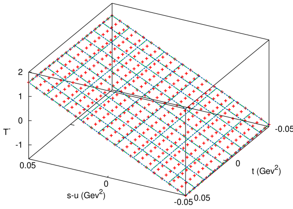
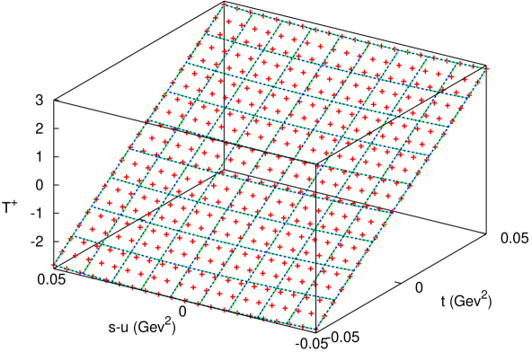
The fit of the subthreshold expansion (14) to the ChPT NNLO result is shown in Figs. 2 and 2 (notice there are three surfaces in each plot) and the resulting to be subtracted threshold parameters are shown in Tabs. 2 and 2.

Figure 1: $T^{+}$ as a function of $t$ and $s-u$. Red points are numerics generated with $L_{i}$s$=$fit10 and $C_{i}$s$=0$. Fitting is with $\sum_{i}\sum_{j}c^{+}_{ij}t^{i}\nu^{2j+1}$. Blue surface: $i+2j\leq 5$. Green surface: $i+2j\leq 4$

Figure 2: $T^{-}$ as a function of $t$ and $s-u$. Red points are numerics generated with $L_{i}$s$=$fit10 and $C_{i}$s$=0$. Fitting is with $\sum_{i}\sum_{j}c^{+}_{ij}t^{i}\nu^{2j+1}$. Blue surface: $i+2j\leq 5$. Green surface: $i+2j\leq 4$

Subthreshold parameters ($C_{i}$s$=0$, $L_{i}$s$=$fit10)
$10c^{+}_{00}$	$-0.709$	$c^{+}_{10}$	$1.101$
$10^{2}c^{+}_{20}$	$-0.485$	$c^{+}_{01}$	$3.467$
$10^{2}c^{+}_{30}$	$0.186$	$c^{+}_{11}$	$-0.131$
$10^{3}c^{+}_{40}$	$0.250$	$10^{2}c^{+}_{21}$	$0.824$

Table 1: Values of $c^{+}_{ij}$ (in unit of $m^{2(i+j)}_{\pi}$) from fit with $i+2j\leq 5$ (see Figure 2)

Subthreshold parameters ( $C_{i}$s$=0$, $L_{i}$s$=$fit10)
$c^{-}_{00}$	$8.398$	$10c^{-}_{10}$	$0.959$
$10^{2}c^{-}_{20}$	$0.791$	$c^{-}_{01}$	$0.426$
$10^{4}c^{-}_{30}$	$-1.04$	$10^{2}c^{-}_{11}$	$-6.04$

Table 2: Values of $c^{-}_{ij}$ (in units of $m^{2i+2j+1}_{\pi}$) from fit with $i+2j\leq 5$ (see Figure 2 ).

Using the results of Tab. 2 we get for the to be subtracted part of the relation (15):

$$\frac{F^{6}_{\pi}}{m^{3}_{\pi}}(1.582)\iff\frac{F^{6}_{\pi}}{m^{3}_{\pi}}(1.278)\,.$$ (25)

The dispersive analysis [10] gives the experimental results for both sides of (15)

$$\frac{F^{6}_{\pi}}{m^{3}_{\pi}}(1.70\pm 0.02)\iff\frac{F^{6}_{\pi}}{m^{3}_{\pi}}(1.9\pm 0.18)$$ (26)

The difference (26)$-$(25) is what should satisfy (15):

$$0.12\pm 0.02\stackrel{{\scriptstyle\textstyle?}}{{=}}0.6\pm 0.18$$ (27)

As you see in (27) the right and the left hand side are not in agreement. Probably it is the same discrepancy found between ChPT [4], $c^{-}_{20}=0.013$, and dispersive results [10] $c^{-}_{20}=0.0085\pm 0.0001$ noticed before [4]. This is related to the conflicting $C_{i}$ determinations in [13].

3.2 $K_{l4}$

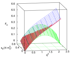
We now do the same analysis for $F_{s}$. As shown in Figure 3 we performed two fits with different degree polynomials. The higher degree fits better the dependence on $s_{\ell}$ even thought in the region probed experimentally in [11] $(\frac{s_{\ell}}{4m^{2}_{\pi}}\leq 0.4\textrm{ and }q^{2}\leq 1)$ the lower degree polynomial fits well. $f_{s}$ and $f_{e}$ turns out to be in agreement between the two fits. We quote here the results for the blue fit. The uncertainties are a measure on how much the two fits differ:

Figure 3: $F_{s}$ as a function of $\frac{s_{\ell}}{4m_{\pi}}$ and $q^{2}$. Red point are numerics generated with $L_{i}=$fit10 and $C_{i}=0$. Green surface: fit with $f_{s}(1+\frac{f^{\prime}_{s}}{f_{s}}q^{2}+\frac{f^{\prime\prime}_{s}}{f_{s}}q^{4}+\frac{f_{e}}{f_{s}}\frac{s_{e}}{4m^{2}_{\pi}})$. Blue surface: fit with $f_{s}(1+\frac{f^{\prime}_{s}}{f_{s}}q^{2}+\frac{f^{\prime\prime}_{s}}{f_{s}}q^{4}+\frac{f^{\prime\prime\prime}_{s}}{f_{s}}q^{6}+\frac{f_{e}}{f_{s}}\frac{s_{e}}{4m^{2}_{\pi}})$

$$f_{s}=5.924\pm 0.002\quad\frac{f^{\prime}_{s}}{f_{s}}=0.075\pm 0.005\quad\frac{f^{\prime\prime}_{s}}{f_{s}}=-0.03\pm 0.009\quad\frac{f^{\prime}_{e}}{f_{s}}=0.038\pm 0.002$$ (28)

Using the value (28) for $f^{\prime\prime}_{s}$, Tab. 2 for $c^{+}_{31}$ we get for the to be subtracted part for the relation (19)

$$-0.049\pm 0.002\iff 0.0521\pm 0.0006\,.$$ (29)

The experimental results of [11] (value for $f_{s}=5.77$ from [12]) and  [10] give the experimental part:

$$-0.14\pm 0.04\iff 0.09\pm 0.02\,.$$ (30)

The difference (30)$-$(29) is:

$$-0.08\pm 0.04\stackrel{{\scriptstyle\textstyle?}}{{=}}0.04\pm 0.02\,.$$ (31)

Again a discrepancy shows up: now the two sides of the relation (19) have opposite sign.

4 Conclusions

We have presented here the first results of search for relations at NNLO in ChPT that are independent of the order $p^{6}$ LECs. We found several previously unknown relations and have presented preliminary numerical results for two of them.

References

• [1] G. Amorós, J. Bijnens and P. Talavera, Nucl. Phys.  B 602 (2001) 87 [hep-ph/0101127].
• [2] J. Bijnens, Prog. Part. Nucl. Phys.  58 (2007) 521 [hep-ph/0604043]; J. Bijnens, talk at this conference.
• [3] G. Amorós, J. Bijnens and P. Talavera, Nucl. Phys.  B 585 (2000) 293 [Erratum-ibid.  B 598 (2001) 665] [hep-ph/0003258].
• [4] J. Bijnens, P. Dhonte and P. Talavera, JHEP 0405 (2004) 036 [hep-ph/0404150].
• [5] J. Bijnens, G. Colangelo, G. Ecker and J. Gasser, hep-ph/9411311.
• [6] G. Amorós and J. Bijnens, J. Phys. G 25 (1999) 1607 [hep-ph/9902463].
• [7] J. Gasser and H. Leutwyler, Nucl. Phys.  B 250 (1985) 517.
• [8] J. Bijnens and P. Dhonte, JHEP 0310 (2003) 061 [hep-ph/0307044].
• [9] J. Bijnens and P. Talavera, Nucl. Phys.  B 669 (2003) 341 [hep-ph/0303103].
• [10] P. Buettiker, S. Descotes-Genon and B. Moussallam, Eur. Phys. J.  C 33 (2004) 409 [hep-ph/0310283].
• [11] J. R. Batley et al. [NA48/2 Collaboration], Eur. Phys. J.  C 54 (2008) 411.
• [12] S. Pislak et al. [BNL-E865 Collaboration], Phys. Rev. Lett.  87 (2001) 221801 [hep-ex/0106071].
• [13] K. Kampf and B. Moussallam, Eur. Phys. J.  C 47 (2006) 723 [hep-ph/0604125].