Parametric analysis of RNA folding
Abstract
We extend recent methods for parametric sequence alignment to the parameter space for scoring RNA folds. This involves the construction of an RNA polytope. A vertex of this polytope corresponds to RNA secondary structures with common branching. We use this polytope and its normal fan to study the effect of varying three parameters in the free energy model that are not determined experimentally. Our results indicate that variation of these specific parameters does not have a dramatic effect on the structures predicted by the free energy model. We additionally map a collection of known RNA secondary structures to the RNA polytope.
Keywords: RNA secondary structure; plane tree; free energy; thermodynamic model; parametric analysis
1 Introduction
Determining the structure of RNA molecules remains a fundamental scientific challenge, since current methods cannot always identify the “correct” fold from the large number of possible configurations. A common method for predicting the secondary structure of a single RNA molecule, termed the thermodynamic model, involves free energy minimization [21, 32, 34]. Extensions to this approach, such as suboptimal structure prediction and partition function calculations, still depend on the parameters from the thermodynamic model to score possible secondary structures. The free energy of a secondary structure is calculated by scoring substructures according to a set of parameters—most of which are determined experimentally (see [16] for a review). A dynamic programming algorithm, used in software packages like mfold [20, 33], computes the minimal free energy as well as the optimal secondary structure(s) [19].
In this work, we address variation in the parameter space for scoring secondary structures, focusing on three parameters from the multi-branch loop energy function that are not based on measurement. Specifically, we address the following questions. What is the geometry of the parameter space for scoring RNA folds and how does this geometry relate back to the biology? How sensitive is the thermodynamic model to variation of the ad-hoc multi-branch loop parameters? We answer these questions using geometric combinatorics. We find that variation of the multi-branch loop parameters has a smaller effect than the change in the parameter space coming from improved measurement. Moreover, regardless of the choice of multi-branch loop parameters used in the current version of the thermodynamic model, the minimal energy structures have a low degree of branching.
Our results are achieved by applying techniques from geometric combinatorics to give a parametric analysis of RNA folding. We construct an RNA polytope whose vertices correspond to sets of secondary structures with common branching. Its normal fan subdivides the parameter space so that the parameters lying in the same cone give the same minimal free energy structures. These approaches have been used recently in parametric sequence alignment [7, 8, 22] and for more general hidden Markov models [4, 23]. There is also earlier polyhedral work on parametric sequence alignment [13, 30] and related work on secondary structure comparison [29] and sequence/structure alignment [18]. We additionally make comparisons with biological structures, and this work supports our theoretical results.
2 Background
2.1 Plane trees and RNA folding
We use a simplified model of RNA folding in which a secondary structure is represented by a rooted plane tree . Single-stranded RNA sequences fold into molecular structures. One step in this folding process is the formation of Watson-Crick and also G-U base pairs. The set of (nested) base pairs determines the secondary structure of an RNA sequence. As illustrated in Figure 1, a secondary structure has two basic types of substructures—runs of stacked base pairs which are called helices and the single-stranded regions known as loops. Every component of a secondary structure is given an associated free energy score by the thermodynamic model. To a first approximation, the score of a loop is determined its degree—the number of base pairs contained in the loop. There are different energy functions for the external loop, hairpin loops, which have degree , bulge/internal loops with degree , and multi-branch loops with degree greater than . Suppose is multi-branch loop, then the free energy of is
| (1) |
where is the number of single-stranded bases in , is the number of helices in , is the sum of the single-base stacking energies in , and are the parameters for offset, free base, and helix penalties, respectively [34]. In this work, our analysis is primarily focused on the three parameters and from this function since they are not experimentally determined. Our results are obtained by considering rooted plane trees as a simplified model of RNA folding.
Plane trees have been used to enumerate possible RNA secondary structures [24] and also to compare them [17, 25] for some time now. The interaction between combinatorics and RNA folding has continued to develop over the last 20 years, including using trees as more abstract representations of RNA folding, for instance in [11] and related work as well as in [2, 3, 14]. A rooted plane tree (also called plane tree or ordered tree [5, 27]) is a tree with a specified root vertex and such that the subtrees of any given vertex are ordered. This ordering comes from the linear arrangement of the RNA sequence. Plane trees with edges are one of the many combinatorial objects counted by the Catalan numbers
| (2) |
To obtain , we assign the root vertex to the exterior loop of and the non-root vertices of correspond to the remaining loops in . Two vertices in share an edge when their loops in are connected by helices. As an example, we give a secondary structure in Figure 1A together with its associated plane tree in Figure 1B. Technically, a secondary structure must be free of pseudoknots in order to construct . While pseudoknots do occur in secondary structures, the thermodynamic model cannot predict them and moreover one can create a nested, pseudoknot-free structure from a given fold in several ways—some of which are in [26] and our approach is described the Materials and Methods section.
A)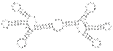 B)
B) 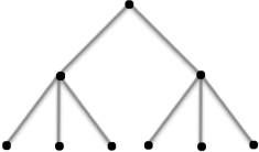
Given a plane tree with edges, we write for the degree of the root vertex and for , is the number of non-root vertices with children. Thus, gives the number of non-root vertices in with degree , and this is the number of loops in with branches. To assign an energy to a plane tree, we assign weights to the vertices, based on the down degree of the vertex. In terms of secondary structures, we are assigning the same energy to each type of loop in the fold. This is a simplification of the scoring for the thermodynamic model, in which the energy of a structure is the sum of the energies of the loops. If is a plane free with edges, the free energy of is written as
where we have used the relations
that hold for all plane trees [27]. To minimize free energy, we must minimize over the space of all plane trees. Since this space is infinite, we will typically think of as being fixed but arbitrary and minimize the free energy function over the finite space of plane trees with edges. For a given set of parameters , this is equivalent to minimizing the following inner product
| (3) |
where
2.2 Geometric combinatorics
In this section, we present some basic definitions in geometric combinatorics. We refer the reader to [12, 31] for a more detailed treatment. A set is convex if for any two points , the line segment connecting and is contained in , that is . For any subset of , the convex hull of , written , is the intersection of all convex sets that contain . A lattice polytope is the convex hull of a finite collection of lattice points: , where .
Any lattice polytope is characterized by a finite collection of defining inequalities
| (4) |
A face of is a subset defined by setting some of the defining inequalities to equality, i.e.
and the dimension of is the dimension of its affine span. The vertices of are the -dimensional faces while the facets have dimension . The boundary of , written is the union of all faces of of dimensions .
A convex polyhedral cone is the positive hull of a finite collection of lattice points in : , and we write . Associated to each lattice polytope is its normal fan that is a collection of cones and subdivides . The rays (-dimensional cones) of are of the form for in (4). Moreover, the cones are in one-to-one correspondence with faces of :
| (5) |
Note that . In terms of minimization, equation (5) states that the points in are minimizers of the dot product for vectors in , among all points in . As an example of the above concepts, we give a -dimensional polytope in Figure 2A and its normal fan in Figure 2B. The four vertices of correspond to the four -dimensional cones in , and the four facets of correspond to the four rays of .
A)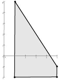 B)
B) 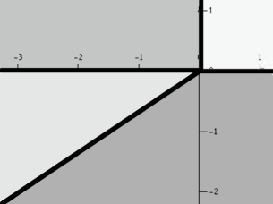
3 Results
3.1 Plane trees that minimize energy
Fixing , the possible count vectors of plane trees are classified by the second author [14] and fall into one of four classes, as listed in Table I with in all cases.
| Set of inequalities | Vertices for even | Vertices for odd | |
|---|---|---|---|
| (A) | |||
| (B) | |||
| (C) | |||
| (D) |
Since must all be integers, the vertices in Table IB or Table ID differ depending on whether or not is even or odd. We want to minimize the linear energy function over this point set (which includes count vectors from all four cases), and hence we let be the convex hull of the union of the four polytopes listed in Table I. Regardless of our choice of energy parameters, a minimum energy plane tree with edges will occur at a vertex of . The following proposition describes the vertices of .
Proposition 3.1.1.
Define as follows.
Then for .
Proof.
Clearly and hence we’ll show each lattice point of in Table I is contained in . The normal fan of has rays
Moreover, for each lattice point in Table I, one can verify that satisfies the defining inequalities of :
and for even we additionally have
This gives , and we have equality. ∎
In the sequel, we will primarily focus on the rational tetrahedron
regardless of whether is even or odd. There are many reasons for this. First, asymptotically, there is no difference between and for even. The normal fan is obtained from by adding a single ray and subdividing the full dimensional cone corresponding to the vertex . Thus, when is even, the parameters giving or the minimal energy are the same regardless of whether we use the subdivision of determined by or that determined by . Moreover, the parameters in will yield or as minimal, and the trees corresponding to these three count vectors are all similar, as discussed in Proposition 3.3.1.
3.2 Lattice points in
Suppose is a secondary structure whose plane tree has count vector . If then there is no choice of parameters that can make have minimal free energy. Conversely, if for some face of , then any parameter vector in the cone yields with minimal energy. We thus want to determine the count vectors lying on .
All four sets of inequalities in Table I intersect . Let , , , and be the polyhedra described in Table IA, IB, IC, and ID, respectively. Then, and
Since is -dimensional, it cannot be contained in the boundary of . We do, however, have
| (6) |
where , , and . Equation (6) follows from counting lattice points in the objects on the left and right hand sides of the equation using the same technique as in Proposition 3.2.1. The plane trees defined in Table ID that lie on satisfy or . Their associated secondary structures either have no bulges/internal loops or have a maximal number of helices in the exterior loop.
Next, we count the number of lattice points in the interior of each face of . For an edge of the form , we use the formula
and obtain the following counts. The edges and each have lattice points in their interiors. A total of lattice points are in the interior of . The interior of contains lattice points, and there are no interior lattice points for the edges and .
To determine the number of lattice points in a facet of , we use Pick’s theorem [15]
where the area of is normalized with respect to the -dimensional sublattice containing . We illustrate Pick’s theorem with the following proposition.
Proposition 3.2.1.
There are no interior lattice points in the facet
Proof.
The triangle lies on the hyperplane in , and thus we normalize the area of by dividing by . Before normalization, the area of is
Moreover, using the counts above for the interior lattice points in the edges of , we have
Applying Pick’s theorem yields
∎
For the other three facets of , each contains interior lattice points. In total, this gives lattice points on , all of which correspond to plane trees.
3.3 Biological meaning of and
3.3.1 The vertices of
The vertices of represent the secondary structures with the maximum number of helices in a loop—so-called “maximal degree of branching”—and the fewest helices in a loop—or “minimal degree of branching”—as described below.
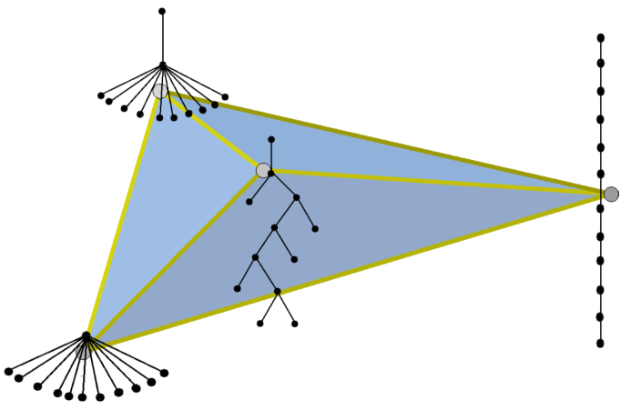
If is a plane tree represented as a vertex of then has edges and vertices. If in addition, has count vector then the degree of the root vertex is and the vertices are the root together with the leaves (vertices with children). Thus, a secondary structure corresponding to has no internal loops, bulges, or multi-branch loops and the exterior loop has helices.
If has count vector , the root vertex has degree , there is one leaf, and vertices of degree ( child). Thus, is a straight line, and a secondary structure corresponding to has no multi-branch loops and the exterior loop has one helix..
If has count vector , the vertices are the root (with degree ), leaves, and one vertex of degree . Secondary structures corresponding to have no internal loops or bulges and one multi-branch loop with helices. In addition, the exterior loop has one helix.
The remaining vertices— for odd and , , or for even—are dealt with in the following proposition.
Proposition 3.3.1.
-
(i)
For odd, any plane tree with count vector satisfies and for .
-
(ii)
For even, any plane tree with count vector or satisfies and for .
-
(iii)
For even, any plane tree with count vector satisfies and for .
Proof.
For (i), suppose is odd and is a plane tree with edges, , , and . Then, has vertices of degree , and the remaining vertices have degree at least . Thus,
However, since , we must have equality. Thus, all other vertices must have degree ( children).
For (iii), a plane tree with edges, , and has vertices of degree and zero vertices of degree . Such a tree cannot have all other vertices of degree as this would yield a graph with an odd number of odd vertices. Thus, there is a vertex with degree with even. This gives
As before this inequality must be an equality, and hence and all other vertices have degree . ∎
Thus, for odd, the count vector corresponds to secondary structures with no interior loops/bulges, all multi-branch loops have helices, and the exterior loop has one helix. When is even, a secondary structure with helices and all three of these properties is not possible. We instead have three cases, each with exactly one of the properties relaxed: a structure corresponding to has one interior loop/bulge, the count vector arises from structures having one multi-branch loop with helices (all other multi-branch loops have helices), and the exterior loop of a structure corresponding to has helices. For odd, plane trees representative of those described in this section are shown in Figure 3.
Remark.
The map from plane trees to count vectors is generically many-to-one. Three of the vertices, however, correspond to exactly one tree: . The trees with count vector are in one-to-one correspondence with full binary trees with edges (by removing the root vertex). There are such trees [6], where is the th Catalan number defined in equation (2).
3.3.2 The rays in
The energy function in equation (3) scores a secondary structure with helices based on the number of helices in the exterior loop, the number hairpin loops, and the number of bulges/internal loops. The normal fan of subdivides the parameter space. Each vector in corresponds to a scoring function in which gives the weight of a helix in the external loop, gives the weight of a hairpin loop, and gives the weight of a bulge/internal loop.
The fan consists of cones generated by elements in the power set
Thus, a parameter vector has the form with and . A generic vector in lies in the interior of one of the -dimensional cones in , and hence we give a brief interpretation of the parameter vectors with for .
Scoring vectors in the interior of the cone penalize for hairpin loops and can independently penalize or reward for helices in the exterior loop and bulges/internal loops. If then gives a penalty for both hairpin loops and interior loops/bulges. Helices in the exterior loop can be beneficial or harmful with this scoring vector, and can equally penalize helices in the exterior loop, hairpin loops, and internal loops/bulges. Scoring vectors in the interior of one of the two remaining cones can reward or penalize all three quantities. These are not independent, however. For instance, if and hairpin loops are disadvantageous under ’s scoring scheme then helices in the exterior loop are beneficial. If and rewards hairpin loops then rewards bulges/internal loops. Similarly, if penalizes for bulges/internal loops then penalizes for hairpin loops. Also, scoring vectors in the interior of the cone can equally reward hairpin loops, internal loops/bulges, and helices in the exterior loop.
3.4 Variation in the parameter space
In this section, we add additional information to the parameters in order to study the effect of varying the multi-branch loop parameters in the thermodynamic model of RNA folding. We obtain free energy parameters for plane trees using one of the four combinatorial sequences having the form
In these sequences, the segments of the form pair with the segments while the nucleotides remain unpaired, and moreover all the loops of a given type have the same free energy. We do not include the possibilities and or and because we want to prevent the pairing. For a given sequence, we use both the current (version 3.0) [19] and previous (version 2.3) [28] thermodynamic parameters, determined by the Turner lab. The parameters and are based on experimental measurement and are listed in Table II. The parameters and come from the multi-branch loop scoring function in equation (1), where the parameters , and in this function are not determined experimentally. If is a multi-branch loop with single-stranded bases and helices and appears in a secondary structure for one of our combinatorial sequences, then we have . Additionally, for each helix in , the single-base stacking energy is . Thus, free energy of in equation (1) becomes , and the parameters and in the free energy function in equation (3) can be written as and .
| Turner 3.0 Values | Turner 2.3 Values | |||||
|---|---|---|---|---|---|---|
| Sequence | ||||||
| X=A, Y=G, Z=C | ||||||
| X=A, Y=C, Z=G | ||||||
| X=C, Y=A, Z=U | ||||||
| X=C, Y=U, Z=A | ||||||
Table III illustrates three types of variation: variation of specific nucleotides in combinatorial sequence, variation of the version of Turner’s energy parameters, and variation of parameters. The effect of varying the multi-branch loop parameters is more or less the same for each sequence and energy table: two different count vectors can be minimal depending on the value of . Technically, a third vertex of has minimal energy in some cases when . However, if the offset and helix penalties are both zero, the multi-branch energy function will have no penalties for the number of single-stranded bases and the number of stems in a loop. This does not agree with the free energy model.
Varying the sequence alone, we obtain differences in the cut-off values for . On the whole, however, nucleotide variation in the combinatorial sequence does not give qualitative differences in the minimal energy plane trees.
We do see (in of the sequences) qualitative differences in the minimal energy trees when we compare version 3.0 parameters to version 2.3 parameters. For instance, when is large, of the sequences give the ‘straight line’ tree with count vector minimal with version 3.0 parameters. Using version 2.3, all four sequences result in the maximal degree of branching, with count vector having minimal energy. This difference in minimal energy trees is not too surprising because the change from version 2.3 to version 3.0 was based on more accurate experimental measurement. The secondary predicted structures have indeed changed.
| Vertex | Rays in | Energy version | Restrictions on | |
|---|---|---|---|---|
It is worth noting that if we use the actual penalties for offset, free base, and helix from versions and of the Turner energies, we obtain
Thus, all four combinatorial sequences yield with minimal energy for version . Moreover, as 9.7 is a fair amount greater than the cut off for all four sequences, slight variation in these parameters will not change the predicted structure. For version , the two combinatorial sequences with unpaired poly-A segments have being minimal while is minimal for the other two sequences. Also, 4.6 is much closer to the cut off values for the sequences. Small changes in these parameters could change which trees have minimal energy.
3.5 RNA STRAND database analysis
3.5.1 Overall shape of data
Our initial collection of secondary structures contains structures from distinct RNA sequences, as described in Materials and Methods. The sequences range from to nucleotides. We exclude structures for which the number of helices is less than from further analysis. This reason for this is that not all the vertices of listed in Proposition 3.1.1 are valid and distinct when . We have structures with (from sequences) having average (median) length of and . We break these into classes, based on the number of helices, as depicted in Table IV.
While our collection contains more small and medium trees as compared to large trees, this reflects the frequency in the RNA STRAND database. For instance, according to an analysis done by RNA STRAND, the average (median) number of helices over the entire database is . This count does, however, include the sequences with fewer than helices and includes a less restrictive definition of bulges/internal loops and helices: internal loops/bulges can have any number of unpaired bases and helices can have any number of base pairs. Our large trees come from S ribosomal RNA and S ribosomal RNA sequences and have a minimum sequence length of nucleotides. In the RNA STRAND database, only % of the structures contain at least nucleotides.
| Category | Range of | # of trees | Average length | Median length | Average | Median |
|---|---|---|---|---|---|---|
| Small | ||||||
| Medium | ||||||
| Large |
3.5.2 Location of count vectors on polytope
It is of great importance to know when biologically correct secondary structures can be predicted by the free energy model. With our simplified energy function in (3), we ask if the biologically correct structures can be minimal for some choice of parameters. As mentioned in §3.2, this translates into determining when the corresponding count vectors lie on the boundary of .
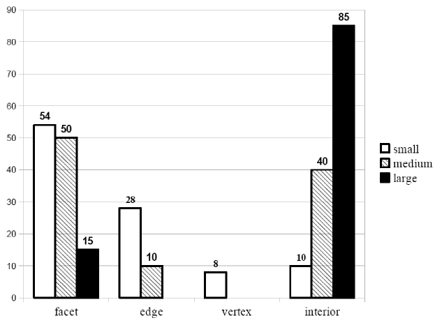
Seventy-one out of 110 count vectors lie on the boundary of : lying on the interior of a facet, lying on the interior of an edge, and occurring as vertices. The average number of edges for plane trees on the boundary of is and is for plane trees in the interior of . Of those contained in the interior of a facet, are minimal for parameters in , are minimal for parameters in , and are minimal for parameter values in . Of those contained in the interior of an edge, are minimal for parameters in , are minimal for parameters in , and is minimal for parameters in . The count vectors that are vertices of satisfy or and consist of the set . Figure 4 shows the location of the count vectors for small, medium, and large trees, given in terms of the percentage of trees in each category.
3.5.3 Closest vertex to count vectors
In order to determine which of the vertices of is closest to a given count vector, we map the tetrahedron
onto the standard tetrahedron with vertices . This is accomplished with the following matrix
| (8) |
which has determinant . For a given , any count vector can be written as a sum
with and . After applying the linear transformation (8), the lattice point will have coordinates . The coordinate gives a measure of the ‘closeness’ to vertex . For a given RNA structure, the largest of the gives the vertex closest to its count vector. Moreover, if then .
Fifty-two of the structures are closest to , are closest to , are closest to , and are closest to . Additionally, we have that are closest to both and and that are closest to both and . The average values of over the structures are which shows that as a whole, the count vectors are closest to and .
We say a count vector is ‘close’ to vertex if The value is halfway in between the smallest and largest possible values of . With this definition, of the small trees are close to vertices, of the medium trees are close to vertices, and no large trees are close to vertices. Thirteen trees in total are close to vertices, of which are close to , are close to , are close to , and is close to . All thirteen of these lattice points lie on the boundary of and hence correspond to minimal energy trees for some choice of parameter values.
4 Discussion and Conclusions
We have used a simple scoring scheme for scoring RNA folds: energy is assigned to a secondary structure based solely on the total number of helices, the number of helices in the exterior loop, and the numbers of hairpin loops and bulges/internal loops. Fixing the total number of helices, the extremal folds are those with the maximal and minimal degrees of branching. When a generic parameter vector is chosen, precisely one of those will have minimal energy. For more specific choices of parameters (biologically realistic or not), the number of minimal count vectors is on the order of the square of the total number of helices. While this seems large, the total number of count vectors that cannot be minimal for any choice of parameters is on the order of the cube of the total number of helices. Thus, when this total is large, we would not expect such a scoring scheme to accurately predict the correct structures. This is supported by our RNA STRAND analysis in which of the count vectors from known structures with a high number of helices cannot be minimal for any choice of parameters. None of these structures are ‘close’ to the extremal folds. This is not unexpected, however, since even the highly detailed free energy model is not accurate for large RNA molecules [9].
On the other hand, when the total number of helices is small, only of the known structures cannot be minimal for our scoring scheme. While the scoring function used in this work is too simplistic to implement in a prediction software, our results suggest that for small RNA molecules, the full free energy model is not necessary for accurate predictions. We are not the first to make this observation, for [10] analyzed some simple probabilistic RNA folding models—one with as few free parameters—whose accuracies are comparable to mfold’s. In their study, the sequences used for testing came from ribonuclease P RNA, transfer mRNA, and signal recognition particle RNA sequences, all of which yield small to medium trees by our classification. While parameters is far too many for parametric analysis using polyhedral geometry, perhaps a simple model incorporating some thermodynamics and some probabilistic parameters can accurately predict the folding of small RNA molecules.
We compared the variation of multi-branch loop parameters to two other types of variation in the parameter space. Fixing the combinatorial sequence and energy version, two possible count vectors can be minimal by varying the multi-branch loops parameters. If we use the most recent (accurate) energy version, we find that for 3 of the 4 sequences, these two count vectors include and . Interestingly, these two vertices are closest to the known structures in our RNA STRAND collection. Moreover, regardless of the choices of multi-branch loop parameters in the current version of the thermodynamic model, predicted structures have a low degree of branching—both in the exterior loop and in the multi-branch loops. Out of the three possible variations, the most significant changes come from varying the energy version, as the possible predicted structure for version 2.3 have a high degree of branching. Even though the penalties for off-set, free base and helix in the multi-branch loop energy calculation are chosen without specific measurement, they do not appear to have a dramatic effect on the predicted structures. One would hope that the parameters determined experimentally are what truly govern the predicted structures, and our findings support this possibility.
5 Materials and Methods
5.1 Selection of secondary structures from RNA STRAND database
The RNA STRAND database [1] was searched by type of RNA (for example, S ribosomal RNA, cis-regulatory element, or group I intron). Each type of RNA was sorted by molecule length, and structures were selected from a variety of organisms to be representative of the different lengths appearing in the database for that type of RNA. Visual inspection of the secondary structures was important in the selection of the structures for our collection. It allowed for the inclusion of similar length structures with different types of branching. It also prevented our collection from containing nearly identical structures formed by two different RNA molecules of the same type. Finally, visual inspection kept our collection from having a plethora of structures with only one or two helices; these structures are overrepresented in the RNA STRAND database.
5.2 Removal of pseudoknots from .ct files
In order to obtain a plane tree from a give secondary structure, pseudoknots were removed. A perl script read the .ct file and stored the closing pairs of all helices, where the helices are defined is §5.3. Each pair and of closing pairs was tested to see if . If true, the pairs and were printed to a file. Next, for each pair and in the output file, one of the associated helices was removed according to the following rubric. If some closing pair appears multiple times, its helix was removed under the assumption that it formed a pseudoknot. If both and were not listed with any other closing pairs, the shorter of the corresponding helices was removed. In the event that the two helices had the same number of paired bases, two versions of the .ct file were saved—one with the first helix removed and one with the second helix removed.
5.3 Calculation of from .ct files
After all the pseudoknots were removed from the .ct files of secondary structures in our collection, a perl script calculated and . In our simplified model of RNA folding, all helices have the same energy independent of the number of base pairs in the helix. Similarly, all bulges/internal loops have the same energy regardless of the number of free bases in the loop. Because of this, very small bulges/internal loops and very short helices were ignored. Bulges and interior loops were required to have at least unpaired bases. No restrictions were placed on the number of free bases in a hairpin loop, which was important so as to maintain the graph structure (edges connecting two vertices).
A)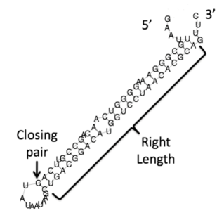 B)
B)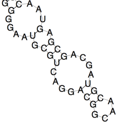 C)
C) 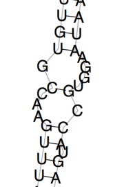
Each helix with choice of closing pair has a ‘left length’ and ‘right length’ of the helix. The left length of a helix is the number of bases in the portion of the sequence that terminates at one of the closing bases. The right length of a helix is the number of bases in the portion of the sequence that originates at one of the closing bases. The closing pair of a helix as well as its right length are depicted in Figure 5A. For this structure, the helix with closing pair G–C has left length and right length . For our analyses, a helix was defined to have both the left and right length or greater. Thus, the piece of secondary structure shown in Figure 5B has two helices—one with left and right length and one with left and right length —and one hairpin loop. Similarly, with our definitions, the fragment depicted in Figure 5C has only interior loop that contains the base pairs G–C and U–A. The single C–G base pair is not considered a helix, and since each of the internal loops containing the C–G pair have more than unpaired bases, the C–G base pair is not considered a part of either helix.
Acknowledgements
V.H. and C.E.H were both supported by the NIH grant 1R01GM083621-01 (P.I. Heitsch). C.E.H. also acknowledges funding from a Career Award at the Scientific Interface (CASI) from the Burroughs Wellcome Fund (BWF). Additionally, V.H. would like to thank Justin Filoseta for the remarkable computer support at the Georgia Institute of Technology.
References
- [1] M. Andronescu, V. Bereg, H. Hoos, and A. Condon. RNA STRAND: The RNA secondary structure and statistical analysis database. BMC Bioinformatics, 9(1):340, 2008.
- [2] Y. Bakhtin and C. E. Heitsch. Large deviations for random trees. J Stat Phys, 132(3):551–560, 2008.
- [3] Y. Bakhtin and C. E. Heitsch. Large deviations for random trees and the branching of RNA secondary structures. Bull Math Biol, 71(1):84–106, 2009.
- [4] N. Beerenwinkel, C. N. Dewey, and K. M. Woods. Parametric inference of recombination in HIV genomes. preprint available at arXiv:q-bio/0512019v1, Dec 2005.
- [5] N. Dershowitz and S. Zaks. Enumerations of ordered trees. Discrete Math, 31(1):9–28, 1980.
- [6] E. Deutsch. Ordered trees with prescribed root degrees, node degrees, and branch lengths. Discrete Math, 282(1-3):89–94, 2004.
- [7] C. N. Dewey, P. M. Huggins, K. Woods, B. Sturmfels, and L. Pachter. Parametric alignment of drosophila genomes. PLoS Comput Biol, 2(6):606–614, 2006.
- [8] C. N. Dewey and K. Woods. Parametric sequence alignment. In B. Sturmfels and L. Pachter, editors, Algebraic statistics for computational biology, pages 193–205. Cambridge University Press, New York, 2005.
- [9] K. J. Doshi, J. J. Cannone, C. W. Cobaugh, and R. R. Gutell. Evaluation of the suitability of free-energy minimization using nearest-neighbor energy parameters for RNA secondary structure prediction. BMC Bioinformatics, 5(1):105, 2004.
- [10] R. Dowell and S. Eddy. Evaluation of several lightweight stochastic context-free grammars for RNA secondary structure prediction. BMC Bioinformatics, 5(1):71, 2004.
- [11] H. H. Gan, S. Pasquali, and T. Schlick. Exploring the repertoire of RNA secondary motifs using graph theory; implications for RNA design. Nucleic Acids Res, 31(11):2926–43, June 2003.
- [12] B. Grünbaum. Convex polytopes, volume 221 of Graduate Texts in Mathematics. Springer-Verlag, New York, second edition, 2003. Prepared and with a preface by Volker Kaibel, Victor Klee and Günter M. Ziegler.
- [13] D. Gusfield, K. Balasubrama, and D. Naor. Parametric optimization of sequence alignment. Algorithmica, 12(4-5):312–326, 1992.
- [14] C. E. Heitsch. Combinatorial insights into RNA secondary structures. In preparation.
- [15] H. Iseri. An exploration of Pick’s theorem in space. Math Mag, 81(2):106–115, 2008.
- [16] D. H. T. John SantaLucia Jr. Measuring the thermodynamics of RNA secondary structure formation. Biopolymers, 44(3):309–319, 1997.
- [17] S.-Y. Le, R. Nussinov, and J. V. Maizel. Tree graphs of RNA secondary structures and their comparisons. Comput Biomed Res, 22(5):461–473, October 1989.
- [18] H.-P. Lenhof, K. Reinert, and M. Vingron. A polyhedral approach to RNA sequence structure alignment. J Comput Biol, 5:517–530, 1998.
- [19] D. H. Mathews, M. D. Disney, J. L. Childs, S. J. Schroeder, M. Zuker, and D. H. Turner. Incorporating chemical modification constraints into a dynamic programming algorithm for prediction of RNA secondary structure. Proc Nat Acad Sci, 101(19):7287–7292, 2004.
- [20] D. H. Mathews, J. Sabina, M. Zuker, and D. H. Turner. Expanded sequence dependence of thermodynamic parameters improves prediction of RNA secondary structure. J Mol Biol, 288(5):911–940, May 21 1999.
- [21] D. H. Mathews and D. H. Turner. Prediction of RNA secondary structure by free energy minimization. Curr Opin Struct Biol, 16(3):270–278, 2006.
- [22] L. Pachter and B. Sturmfels. Parametric inference for biological sequence analysis. Proc Nat Acad Soc, 101(46):16138–16143, 2004.
- [23] L. Pachter and B. Sturmfels. Tropical geometry of statistical models. Proc Nat Acad Soc, 101(46):16132–16137, 2004.
- [24] W. R. Schmitt and M. S. Waterman. Linear trees and RNA secondary structure. Discrete Appl Math, 51(3):317–323, 1994.
- [25] B. A. Shapiro and K. Zhang. Comparing multiple RNA secondary structures using tree comparisons. Comput Appl Biosci, 6(4):309–18, October 1990.
- [26] S. Smit, K. Rother, J. Heringa, and R. Knight. From knotted to nested RNA structures: a variety of computational methods for pseudoknot removal. RNA, 14(3):410–416, 2008.
- [27] R. P. Stanley. Enumerative combinatorics. Vol. 2, volume 62 of Cambridge Studies in Advanced Mathematics. Cambridge University Press, Cambridge, 1999.
- [28] A. E. Walter and D. H. Turner. Sequence dependence of stability for coaxial stacking of RNA helixes with Watson-Crick base paired interfaces. Biochemistry, 33(42):12715–12719, Oct 25 1994.
- [29] L. Wang and J. Zhao. Parametric alignment of ordered trees. Bioinformatics, 19(17):2237–45, Nov 22 2003.
- [30] M. S. Waterman, M. Eggert, and E. Lander. Parametric sequence comparisons. Proc Nat Acad Sci, 89(12):6090–6093, 1992.
- [31] G. M. Ziegler. Lectures on polytopes, volume 152 of Graduate Texts in Mathematics. Springer-Verlag, New York, 1995.
- [32] M. Zuker. Calculating nucleic acid secondary structure. Curr Opin Struct Biol, 10(3):303–310, 2000.
- [33] M. Zuker. Mfold web server for nucleic acid folding and hybridization prediction. Nucleic Acids Res, 31(13):3406–15, 2003.
- [34] M. Zuker, D. Mathews, and D. Turner. Algorithms and thermodynamics for RNA secondary structure prediction: A practical guide. In J. Barciszewski and B. Clark, editors, RNA Biochemistry and Biotechnology, NATO ASI Series, pages 11–43. Kluwer Academic Publishers, 1999.